RICHARD BRERETON - MULTIVARIATE PATTERN RECOGNITION FOR CHEMOMETRICS - BFR
←
→
Page content transcription
If your browser does not render page correctly, please read the page content below
MULTIVARIATE PATTERN
RECOGNITION FOR CHEMOMETRICS

         Richard Brereton
      r.g.brereton@bris.ac.uk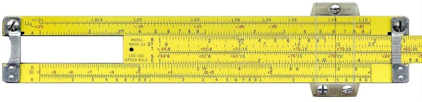
Pattern Recognition

    Book
Chemometrics
  for Pattern
 Recognition,
  Wiley, 2009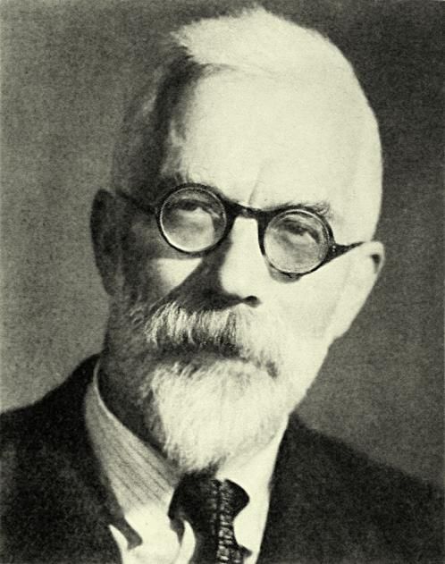
Pattern Recognition
Pattern Recognition
Pattern Recognition

● Many definitions
● Most modern definitions involve classification
● Not just classification algorithms
   o  Is there enough evidence to be able to group samples?
   o  Are there outliers?
   o  Are there unsuspected subgroups?
   o  What are the most diagnostic variables / features / markers?
   o  Is the method robust to future samples with different correlation
      structures?
   Etc.
Pattern Recognition
o Supervised Pattern Recognition
o Known or hypothesised classes in advance
o Majority of applications
o Unsupervised Pattern Recognition
o Class structure not known or hypothesisedHistoric Origins
● 1920s – 1930s
● UK agricultural industry
● Old landowners had to improve
methods after social change
● Statisticians hired to make more
efficient
● R A Fisher and colleagues develop
multivariate methods.
● Early papers eg “Fisher iris data”Historic Origins
● Postwar
● Gradual development and acceptance of
multivariate pattern recognition by
statisticians
● Limited because of computing power
● A 1921 paper by R.A.Fisher calculated to
take
● 8 months of 12 hour days
just to calculate the numbers in the tables at 1
minute per numberHistoric Origins
o 1960s – 1980s
o Chemical Pattern Recognition
o Facile computer power and good programming
languages
o No longer needed to be a statistician
o Origins of chemometrics
o Renamed in mid 1970s by Svante Wold
o The name chemometrics took off in late 1970s / early
1980s
o Early pioneers often regarded themselves as doing
pattern recognition.Historic Origins
o 1980s – 1990s
o Growth of chemometrics
o Pattern recognition small element others such as
o Signal Analysis
o Multivariate Curve Resolution / Factor Analysis
o Experimental Design
o Multivariate Calibration
o Primarily instrumental analytical chemistry
o Often small datasets, eg. 20 samples and 10 HPLC
peaksHistoric Origins
● Modern Day
o Large datasets possible
o Applications to new areas outside mainstream analytical
chemistry
o Cheap and fast computer powerUnivariate Classifiers ● Traditional approach to classification ● Select one or more marker compounds ● Measure o HPLC peak height o GCMS peak height o NMR ● Determine o Presence / absence o Concentration o Peak ratios
Univariate Classifiers

● Traditional approach
● Problems
   o Quantitative analysis is often difficult and very dependent on
       instrument and reference standards.
   o   GCMS, HPLC, extraction may be expensive and time consuming
       whereas spectroscopic methods such as NIR may be faster and
       cheaper
   o   Food contains many compounds and as such using traditional
       methods only a small number of markers are studied
   o   Many differences are quite subtle especially when detecting
       adulteration, different phenotypes, different factories etc.
   o   Some minor differences are important
Multivariate approach
● Multivariate data matrix
VARIABLES
o We measure variables on
samples e.g.
o chromatographic intensities of S
chromatograms A
o concentrations of compounds in M
A sample
reaction mixtures P
o The elements of a matrix consist L
of the size of the measured E
variable in a specific sample e.g. S
o the intensity of a specific peak
in a specific chromatogram
o The intensity of an absorbance An element
by NIR A variable of a matrixMultivariate approach
Classification
ANALYTICAL DATA
o A way of grouping samples
o Predictive modelling
o Predict the origins of S S
samples A A
o Hypothesis tests M M
P P
o Is there a relationship L L
between the analytical E E
signal and their origins? S SModern Chemometrics and
Analytical Chemistry
In the modern word we can obtain many measurements per
sample very easily.
Many methods in textbooks are quite old as there is a long time
lapse between writing texts and accepting new methods, often
20 years.
Much traditional analytical chemistry involves optimisation, can
we get better separations or better efficiencies.
In chemometrics this is not always so: we often do not know
the training set perfectly, there can be outliers, artefacts,
misclassifications or even imperfect techniques.Modern Chemometrics and
Analytical Chemistry
Traditional problems eg Fisher’s iris data, the answer is known for
certainty in advance
The aim is to reach this well established answer as well as we can
We might then ask which variables (in the iris data, the physical
measurements) are most useful (in modern terminology marker
compounds) for example or to predict the origins of an unknown
In many modern situations we do not know the answer in advancePredictive models
Form a mathematical model between the analytical data and
the factor of interest. Can be more than two groups.
ANALYTICAL DATA INFORMATION
S S
Group 1
A A
M M
P P
L L
E E Group 1
S S
MATHEMATICAL MODELPredictive models
Training set
o Traditional approach. Divide samples into
training and test set.
o Develop a method that works very well on
training set.
Weakness
o The training set in itself may not be perfect
o Numerous reasons
o So 95% correctly classified may not
necessarily be “better” than 85%Predictive models Is it possible to predict membership of a group? Can we take an unknown sample and say which group it belongs to using analytical data? Can we classify an unknown sample to a group? Is the data good enough (of sufficient quality)? Are there subgroups in training set? Are there outliers in training set?
Predictive models Can we predict the origins of a food stuff according to its country? By overfitting, yes, but in practice this means nothing. Many examples of “perfect” separation!!!!! With sophisticated modern methods possible but of no meaning
Predictive models
What is the best method?
o No real answer
o Can do on simulations, but these will not incorporate
real life issues
o Simulations good for developing algorithms to check
they work
o In real life we often need controls, eg “null” datasets,
permutationsMultivariate Classification
Techniques
Too much emphasis on named techniques
What matters is formulating the question well
• Choosing an appropriate training set
• Choosing an appropriate test set
• Deciding what problems you will look at
• Eg are you interested in outliers
• Are you interested in distinguishing two or more groups
• How confident are you about the training set
• Is the analytical technique appropriate and reliableClass Boundaries
Classification can be regarded as finding boundaries
between groups of samples. The difference between
techniques corresponds to the difference in establishing
boundaries
● A classifier can be regarded as a method that finds a boundary
between or around groups of samples, all common classifiers can be
defined this way
● All classification methods can be formulated this way, including
approaches based on PLS
● Sometimes techniques are presented in other ways e.g. projection
onto lines, but these projections can be expressed as distance from
boundaries, so the key to all techniques is to find a suitable
boundary. Extensions e.g. class distance plots based on boundaries.Class Boundaries
● Two class classifiers .
o Model two classes simultaneously and try to form a boundary
between them.
● One class classifiers
o Model each class separately. Not all the classes need to be
included.
o Forms boundary around each class that is modelled often at a given
confidence limit.
● Multi class classifiers
o Model several classes simultaneously.Class Boundaries
Class A
Class B
Class B
Class A
Two class classifier Two one class classifiers
Illustrated for bivariate classifiers but can be extended easily to
multivariate classifiersTwo Class Classifiers
● Differ according to the complexity of the boundary
o Model two classes simultaneously and try to form a boundary
between them. Most classifiers can be expressed this way.
● Common Approaches
o Euclidean Distance to Centroids
o Linear Discriminant Analysis
o Quadratic Discriminant Analysis
o Partial Least Squares Discriminant Analysis
o Support Vector Machines
o K Nearest NeighboursTwo Class Classifiers
30 30
20 20
10 10
0 0
PC 2
PC 2
-10 -10
-20 -20
-30 -30
-40 -40
-30 -20 -10 0 10 20 30 40 50 -30 -20 -10 0 10 20 30 40 50
PC 1 PC 1
30 30
20 20
10 10
0 0
PC 2
PC 2
-10 -10
-20 -20
-30 -30
-40 -40
-30 -20 -10 0 10 20 30 40 50 -30 -20 -10 0 10 20 30 40 50
PC 1 PC 1Two Class Classifiers
● No best method
o The more complex boundaries, the better the training set model
o The more complex boundaries, the bigger the risk of over-fitting,
this means mistakes when classifying unknowns
o Often over-optimistic models. So take care!One Class Classifiers
● Forms a boundary around a class
o Usually at a certain percentage probability
o For example 99% means that for a training set group we expect 99
out of 100 samples to be within that boundary.
o Often depends on samples being normally distributed
● Common Approaches
o Quadratic Discriminant Analysis
o Support Vector Domain Description
o Incorporated into SIMCAOne Class Classifiers
0.95
0.75
0.5
0.25 0.99
0.99
0.9One Class Classifiers
.9
95 A0
A 0.95
A
A
0.
B 0.99
0.04
0.
0.
0.2 0.2
9
B 0 .9.9
95
B
0 .9
99
0.04
AB0 09
3
B
0.0 0. 0.0
9
04
0.
5
0.15 0.15 3 04 0.
0. 0.02
.9
B
03
A
0.02
0.
9
0.1 0.1
01
0.
A0
0.0
A 0 A 0 0 .99
0.
0.0
A0
01
0.05 0.05
.95
2
0.01
.9 .9
1
2
.99
0.0
0.03
PC2
PC2
0.03
0.02
9
B 0 .9
A
5
0 0
0.04
B 0 .9
5
0.04
0.01
0.01
.9
A0
B0
.9
-0.05 -0.05
2
0.0
0.0
1
1
0.0
A
-0.1 -0.1 0
02
0 .9A 0 0 .99
.0 0.
2 0.0 0.02
3 3 3
-0.15 -0.15 0.0 0.0 4 0.0
.95
A
9
3 0.0
0 .9
95
0.
9 0.0 4
0.0
4
0.
0.04
B
B
-0.2 B -0.2
-0.2 -0.1 0 0.1 0.2 0.3 -0.2 -0.1 0 0.1 0.2 0.3
PC1 PC1
0.2 0.2
0.15 0.15
0.1 0.1
0.05 0.05
0 0
-0.05 -0.05
-0.1 -0.1
-0.15 -0.15
-0.2 -0.2
-0.2 -0.1 0 0.1 0.2 0.3 -0.2 -0.1 0 0.1 0.2 0.3Multiclass Classifiers
● Extension of two class classifiers
o Simple for some approaches such as LDA or QDA
o Difficult and often misapplied for approaches such as PLS-DA
Class A Class B
Class CComparison of methods There is a large and very misleading literature comparing methods - beware o For example there will be claims that method A is better than methods B, C and D o The method will be claimed to be better as judged by the difference in one or more performance indicator such as %CC (percent correctly classified), usually on a test set and on one or more carefully chosen datasets.
Comparison of methods

o There is strong pressure eg to get PhDs, get grants, get
  papers, or even conference presentations
o Often a method that isn’t “better” is regarded as a waste
  of time, no more grants, papers or PhDs
o Hence there are ever more claims of improved methods
  in the literature and at conferences.
o Beware.
Comparison of methods
It is often not possible to compare methods directly.
o Example
o One class classifiers (eg SIMCA, Support Vector Data
Description, certain types of QDA)
o Two class classifiers (eg LDA, PLS-DA, Euclidean Distance)
Class A Class A
Class B
One class Two classTraditional problems :
comparison of methods
Preprocessing can radically change the performance of
a method
o Example
o PLS-DA is the same as EDC (Euclidean Distance to Centroids) if
only one PLS component is used
o PLS-DA is the same as LDA if all components used
o So we can’t say “we have used PLS-DA” without qualifying this
1 component Several components All non-zero components
PLS-DA=EDC Intermediate PLS-DA=LDATraditional problems :
comparison of methods
Should we use PLS-DA as opposed to statistical
methods?
o The statistical properties eg for LDA (linear discriminant
analysis) and EDC (Euclidean distance to centroids) are well
known and well established.
o A traditional limitation of LDA is that Mahalanobis distance
cannot be calculated if number of variables > number of
samples, but this is not so, just use the sum of squares of
standardised non-zero PCs
o So why use PLS-DA? And why compare to LDA because PLS-
DA could be the same as PLS-DA.Traditional problems :
comparison of methods
Many other choices of parameters for some methods
o Eg PLS-DA
o Data transformation
o Type of centring
o Acceptance criteria
o Number of components
o Etc.
Other methods very little choice
Often the choice of parameters has as much or more
influence than the choice of classification algorithmTraditional problems :
comparison of methods
How to view this
View the classifier just as one step in a series, just like
addition and multiplication but a little more complicated
Focus as much on the data preparation step and
decision making as on the algorithm
We probably have access to all the algorithms we need,
resist trying to invent new ones.
It is often unwise to compare different approaches
directly, and if done, one needs to understand all steps.
The pragmatic approach is to use several quite
incompatible methods and simply come to a
consensus.Conclusions
Historical origins in UK agriculture of the 1920s-30s.
Chemometrics developed in the 1960s-70s
Rapid and easy computing power important
Multivariate advantage
The nature of the problem has changed since the 1970s
Answer often not known for certain in advance
Classifiers are often not comparable
Too much emphasis on named methods and on
comparisons
Much historic software and literature based in 1970s
problemsYou can also read