Neutronics Calculation Advances at Los Alamos: Manhattan Project to Monte Carlo - arXiv

Submitted to ANS Nuclear Technology (2021), LA-UR-21-22202. DRAFT

Neutronics Calculation Advances at Los Alamos: Manhattan Project
to Monte Carlo
 Avneet Sood*, R. Arthur Forster, B.J. Archer, and R.C. Little
 Los Alamos National Laboratory, Los Alamos, NM 87545
 *
 Los Alamos National Laboratory, P.O. Box 1663, MS F663
 *
 E-mail: sooda@lanl.gov

Abstract - The history and advances of neutronics calculations at Los Alamos during
the Manhattan Project through the present is reviewed. We briefly summarize early
simpler, and more approximate neutronics methods. We then motivate the need to better
predict neutronics behavior through consideration of theoretical equations, models and
algorithms, experimental measurements, and available computing capabilities and their
limitations. These, coupled with increasing post-war defense needs, and the invention of
electronic computing led to the creation of Monte Carlo neutronics transport. As a part
of the history, we note the crucial role that the scientific comradery between the great
Los Alamos scientists played in the process. We focus heavily on these early
developments and the subsequent successes of Monte Carlo and its applications to
problems of national defense at Los Alamos. We cover the early methods, algorithms,
and computers, electronic and women pioneers, that enabled Monte Carlo to spread to
all areas of science.

 Keywords: Manhattan Project, Los Alamos National Laboratory, von Neumann,
 Ulam, Metropolis, Fermi, Richtmyer, ENIAC, MANIAC, neutronics, Monte
 Carlo, MCNP

I. THE STATE OF NEUTRONICS CALCULATIONS DURING WORLD
WAR II

I.A. Discovery of Fission
 In December 1938, physicists Lise Meitner and Otto Frisch made a
revolutionary discovery that would forever change nuclear physics and lead the world
into the atomic age: a uranium nucleus had fissioned. The prior discovery of the neutron
in 1932 had created the capability for scientists to probe the atomic nucleus. In 1934,
scientists like Enrico Fermi bombarded large, heavy nuclei with neutrons to produce the
first elements heavier than uranium—or so he thought. The thinking was that hitting a
large nucleus with a neutron could only induce small changes in the number of neutrons
or protons. Other scientist teams like Lise Meitner and her nephew, Otto Frisch,
Austrians exiled in Sweden and Otto Hahn and Fritz Strassmann in Berlin also began
bombarding uranium and other heavy elements with neutrons and found isotopes of
lighter nuclides among the decay products. Meitner and Frisch, using the liquid-drop
model of the nucleus, were able to estimate that approximately 200 MeV would be
required to split a uranium nucleus. Meitner was able to measure the daughter nuclei’s
mass, and show that it was less by about 200 MeV. Meitner and Frisch sent their paper
to Nature in January. Frisch named the process “fission” after observing biologists
describing cell division as “binary fission”. Hahn and Strassmann published their
findings separately. Bohr carried the news of the discovery of fission to America. Other
scientists discovered that the fission reaction also emitted enough secondary neutrons
for a chain reaction along with the release of an enormous amount of energy. As word

Submitted to ANS Nuclear Technology (2021), LA-UR-21-22202

spread, the worldwide scientific community realized the possibility of both making
weapons and getting power from fission. The MAUD report,1 a secret report by British
scientific leaders, warned of the likelihood of producing a weapon if the U-235 isotope
could be separated. The creation of such atomic weapons would have a massive impact
on the war. The MAUD report estimated that a critical mass of 10 kg would be
sufficient for a weapon, small enough to load onto an airplane, and ready in
approximately two years. The MAUD report along with the US Government’s National
Academy of Sciences report helped launch the Manhattan Project and the start of
Project Y, Los Alamos. The race for a weapon was on.2,3

I.B. Early Understanding of Fission
 Enrico Fermi, Frederic Joliot, Leo Szilard, and others independently found
secondary neutrons from fission experiments that they conducted in Paris and in New
York. Weapons applications for fission required the geometric progression of a chain
reaction of fission events. [Serber notes that the term “to fish” was used in place of “to
fission” but the phrase did not stick]. These scientists had an early understanding of how
neutron chain reactions could be used to release massive amounts of energy. The
uncontrolled fissioning of U235 resulting in a massive amount of energy makes the
material very hot, developing a great pressure and thus exploding. Basic equations
characterizing the energy released had been developed but assumed an ideal geometric
arrangement of materials where no neutrons are lost to the surface or to parasitic
absorptions. In realistic configurations, neutrons would be lost by diffusion outward
through the surface. The precise dimensions for a perfect sphere needed to be
determined to exactly balance between the chain reaction of neutrons created by fission
and the surface and parasitic losses. This critical radius would also depend on the
density of the material. An effective explosion depends on whether this balance of
losses occurred before an appreciable fraction of the material had fissioned releasing
enormous amounts of energy in a very short time. Slow, or thermal energy, neutrons
cannot play an effective role in an explosion since they require significant time to be
captured to cause fission.
 Hans Bethe later described assembling fissionable material together and the
resulting complicated shapes. Bethe describes that these problems were insoluble by
analytical means and the resulting equations were beyond the existing desk computing
machines.4
 It wasn’t until early 1945 that Los Alamos received amounts of uranium and
plutonium with masses comparable to their critical mass so that experiments could be
performed to compare with the early predictions. Plutonium and uranium were
fabricated into spheres and shells for comparison with calculations. The critical masses
were determined experimentally by a series of integral experiments. Early critical
experiments were done using reflected geometries.5,6 The critical radius was determined
by plotting the inverse of the observed neutron multiplication as increasingly more
material was added and extrapolating for the point of infinite multiplication. This paper
discusses the various computational methods for solving the neutron transport equation
during the Manhattan Project, the evolution of a new computational capability, and the
invention of stochastic methods, focusing on Monte Carlo, and nuclear data.

I.C. Manhattan Project Advances Solutions to the Neutron Transport Equation
 The earliest estimates for a nuclear bomb were based on natural uranium, and
gave critical masses of many tons. In March 1940 Rudolf Peierls and Otto Frisch used

Submitted to ANS Nuclear Technology (2021), LA-UR-21-22202

diffusion theory to estimate that the critical mass of U235 was less than 1 kg.7 This
estimate persuaded both the United Kingdom and United States to proceed with a
nuclear bomb program. Knowing the critical mass of U235 and Pu239 were essential
for the Manhattan Project for sizing the production plants, and setting safety limits on
experiments. This requirement drove the Los Alamos Theoretical Division (T-Division)
to constantly improve the methods to determine the critical masses.

I.C.1. Neutron Transport Equation
 Estimating the critical masses required solutions to the neutron transport
equation. The neutron transport equation is a mathematical description of neutron
multiplication and movement through materials and is based on the Boltzmann equation
which was used to describe study the kinetic theory of gasses. The Boltzmann equation
was developed in 1872 by Ludwig Boltzmann to explain the properties of dilute gasses
by characterizing the collision processes between pairs of molecules.8 It is a
mathematical description of how systems that are not in a state of equilibrium evolve
(e.g., heat flowing from hot to cold, fluid movement etc.) and can be used to describe
the macroscopic changes in a system. It has terms describing collisions and free
streaming. The general equation looks like:

 + . ∇! + ∇" = , Ω , (Ω)| − ′| ( ′ − )
 
f(r,v,t) is particle distribution and is a function of position (r), velocity (v), and time (t);
F is an external force acting on the particles. The left-hand-side of the equation
represents the free-streaming of particles including the time-rate of change, geometric
losses, and gains from other sources. The right-hand-side of the equation represents the
collisions occurring during the flow. The equation is a non-linear integro-differential
equation involving terms that depends on particle position and momentum.9 A
linearized form of neutron transport equation can be cast into this general Boltzmann
form to describe neutron multiplication and movement through materials.10 The integro-
differential form of the linear, time-dependent neutron transport equation can be written
as:
 (
 1 $ &'
 5 + Ω ∙ ∇ + Σ# 9 = , ′ Σ% + A + , Ω′ , ′ Σ+ + 
 4 4 ' '
 ')*

where = ( , , Ω, ) is the angular neutron flux, = ( , , ) is the scalar neutron
flux, $ , & are the fission and delayed neutron precursor exit energy distributions,
Σ# , Σ+ , Σ% are the macroscopic total, scattering, and fission cross sections and dependent
on , , Ω, , and ' ' are the decay constant and total number of precursor, i, N is the
total number of delayed neutron precursors, and = ( , , Ω, t) source term. The
neutron transport equation is a balance statement that conserves neutrons where each
term represents a gain or a loss of neutrons. The neutron equation states that neutrons
gained equal neutrons lost. The equation is usually solved to find the scalar neutron
flux, , thus allowing for the calculation of reaction rates. Reaction rates can be
measured and are the primary interest in most applications.
 Today this equation can be solved directly by either deterministic or stochastic
methods using advanced algorithms and computational resources. Deterministic
methods are exact solutions everywhere in a problem to an approximate and discretized

Submitted to ANS Nuclear Technology (2021), LA-UR-21-22202

equation. Monte Carlo methods are a statistically-approximate solution to specific
regions of a problem to an exact equation. The techniques are complimentary and can
be used separately or in tandem. The neutron transport equation can be simplified by
making several assumptions allowing for analytic solutions or simple calculations that
could be carried out by the electro-mechanical computers available early in Manhattan
Project. Significant advances in solving simplified versions of the neutron transport
equation were made during this time.

I.C.2. Approximations and Limitations in Diffusion Theory
 Fick’s law states that particles will diffuse from the region of higher flux to the
region of lower flux through collisions. It is valid for locations far (several neutron
mean free paths [mfp]) from the boundaries because of the initial infinite medium
assumption. Additionally, since the neutron flux was assumed to be predominately due
to isotropic scattering collisions, proximity to strong sources or absorbers or any
strongly an-isotropic materials invalidates the original derivations. This invalidation
also includes proximity to any strongly varying material interfaces or boundaries.
Lastly, Fick’s law assumed that the flux was independent of time. Rapid time-varying
flux changes (the time for few mfp collisions) were shown to be the upper limit. Many
of these approximations were not applicable for weapons work but could be useful for a
general predictive capability. Limitations on the methods were understood and better
methods were being developed. Notably, work by Eldred Nelson and Stan Frankel from
the Berkeley theoretical group for a more exact diffusion theory-based solution
dramatically improved the accuracy of solutions.11

I.C.3. Analytic Solutions
 The first improvement in generating analytic solutions came in the late spring of
1942 when Oppenheimer and Serber tasked Stanley Frankel and Eldred Nelson to verify
the British critical mass calculations.3 It turned out that the differential form of the
diffusion equations with realistic boundary conditions was difficult to solve analytically.
At the time, a very general integral equation was being used in broader science
applications to describe physical phenomena and was being mathematically solved. The
integral equation was:

 ( ) = , ′ ( ′) ( ′) (| − ′|)

where r is in one or more phase-space dimensions, F(r) is any general function that is
generally non-zero, K is a kernel, and c is an eigenvalue. The integration is carried out
where F(r) ≠ 0 and solved for N(r) using the smallest eigenvalue, c. F(r) can be of
varying complexity – ranging from a constant value to as complex as a differential
equation (e.g., differential cross sections). The kernel, K, often took common analytic
forms such as the Milne or Gauss kernels describing radiation flow. N(r) was usually
the particle flux. Analytical mathematical solutions to this general equation were being
generated during that time. The neutron transport equation can be cast into this form.
Simplifying assumptions like treating neutrons as mono-energetic, isotropically
scattering in simple geometries, using the same mean free path in all materials make this
equation analytically solvable.
 In 1942 Frankel and Nelson created an analytic solution to this integral form
using what they called the end-point method which they later documented in Los

Submitted to ANS Nuclear Technology (2021), LA-UR-21-22202

Alamos reports.12,13,14 They documented their analytic solutions of this integral equation
and its applications to determine critical dimensions, multiplication rates, with or
without tampers, and probabilities of detonations.15,16 They also show how the integral
equation reduces to the diffusion equation.17 Frankel and Klaus Fuchs compared the
end-point method to the British variation method, and found that they were generally in
agreement.14 Analytic solutions to the neutron transport equation with all of the
simplified assumptions continue to be of use for verification of complicated computer
algorithms.18

I.C.4. Diffusion Theory Critical Mass Estimates
 The purpose of Project Y (The Los Alamos Project) was to build a practical
military weapon that was light enough to carry on an airplane. The preliminary
calculations of the minimum quantity of materials and geometry of such a weapon was
done using an ideal arrangement but quickly advanced to model more realistic
geometries, materials, and combining different areas of physics. The diffusion theory
model of neutron transport played an important role in guiding the early insights to the
geometry and mass needed to achieve criticality.
 Neutron diffusion theory was used as an approximation to the neutron transport
equation during the Manhattan Project. It can be derived from the neutron transport
equation by integrating over angle and using Fick’s Law. Simple diffusion theory treats
neutrons in an infinite medium, at a single energy, and assumes steady-state conditions.
The diffusion equation for neutron transport is:
 * ,-
 " ,#
 = ∇( ∇ ) − Σ. + Σ% + 

or in steady-state:

 0 = ∇/ − Σ. + Σ% + 

 This equation is the basis of the development of neutronics calculations
supporting early Los Alamos efforts. The first term describes the amount of neutron
movement in the material via diffusion coefficient, D. It includes a Laplacian operator
that describes geometry and determines the amount of neutron leakage via surface
curvature. The second term is the loss due to absorption. The last two terms are source
terms from fission and external sources.
 When Serber gave the first lectures at Los Alamos in April 1943 he showed that
using simple diffusion theory, with better boundary conditions extending the distance
where the flux went to zero, gave a critical radius of a bare sphere as:3

 0 = / /( − 1)

where is the mean-time between fissions, is the neutron number from fission, and 
is the diffusion coefficient. The simple and early estimate for the critical radius of U235
was 13.5 cm giving a critical mass of 200 kg. This early estimate of critical mass is
significantly overestimated, a more exact diffusion theory gave a 2/3 reduction. For
U235, this gave rc = 9 cm with a corresponding critical mass of 60 kg which is much
closer to the true value.
 The effects of a reflective material surrounding the core would serve to reflect a
fraction of neutrons that would otherwise escape and therefore reduce the quantity of
fissionable material required for a critical mass. Diffusion theory was applied again and

Submitted to ANS Nuclear Technology (2021), LA-UR-21-22202

showed that the critical mass was 1/8th as much as for a bare system. However, the
approximations in diffusion theory over-estimated the conservation of material masses,
when more accurate diffusion theory emerged it indicated a reduction in the reflected
critical mass of only 1/4th instead of 1/8th.3

I.C.5. Deterministic Solutions
 In deterministic methods, the neutron transport equation (or an approximation of
it, such as diffusion theory) is solved as a differential equation where the spatial,
angular, energy, and time variables are discretized. Spatial variables are typically
discretized by meshing the geometry into many small regions. Angular variables can be
discretized by discrete ordinates and weighting quadrature sets (used in the Sn methods)
or by functional expansion methods such as spherical harmonics (used in Pn methods).
Energy variables are typically discretized by the multi-group method, where each
energy group uses flux-weighted constant cross sections with the scattering kinematics
calculated as energy group-to-group transfer probabilities. The time variable is divided
into discrete time steps, where the time derivatives are replaced with difference
equations. The numerical solutions are iterative since the discretized variables are
solved in sequence until the convergence criteria are satisfied.
 As early as the summer of 1943 it was realized that assuming a single neutron
velocity was not adequate. A procedure was developed using two or three energy
groups for a single material, but it was cumbersome.19,20 In October 1943 Christy used a
three-group approach in predicting the critical mass of the water boiler.21 Feynman’s
group found an easier approach in July 1944 by assuming scattered neutrons did not
change their velocity. This allowed each energy group to be treated individually by
diffusion theory as in multi-group method.19,20,22
 The spherical harmonic method, introduced by Carson Mark and Robert
Marshak, and developed by Roy Glauber in 1944, solved the tamped critical mass
problem for spherical symmetry and one-neutron velocity.22,23 This was quickly
extended to a two-energy group method. After the war Bengt Carlson developed a
matrix version of the spherical harmonics method.22
 In March 1945 Serber introduced an approximation for calculating the critical
mass of a reflected sphere.24,25 The core and reflector could each be described by a
reflection coefficient. The critical mass was determined by matching the two reflection
coefficients. The neutron distribution in the core was approximated by a sinusoidal
form, whereas the reflector neutron distribution was taken as an exponential. The
critical radius could be found from a relatively simple formula. Alan Herries Wilson
(Figure 1) had derived the same formula for spherical reactors in January 1944,26
pointed out to Serber by Kenneth Case.24 Hence, the Serber-Wilson method. Case was
immediately able to apply the Serber-Wilson to several complicated configurations that
had been difficult with the spherical-harmonic method.27 The Serber-Wilson method
was generalized from one neutron energy to multi-group energy.28 The Serber-Wilson
method was the main neutron diffusion method at Los Alamos until it was replaced by
Carlson’s Sn transport method in the late 1950s.

Submitted to ANS Nuclear Technology (2021), LA-UR-21-22202

Figure 1. Sir Alan H. Wilson.29

 In 1953 Carlson first proposed the Sn method, which discretized the angular
variables, for solving the transport equation.31 This was an alternative to the older
spherical-harmonic method. The Sn technique is the deterministic method of choice for
solving most neutron transport problems today. The technique continues to benefit from
past solution techniques to the neutron transport equation. Diffusion Synthetic
Acceleration is one example of a technique that was first developed at Los Alamos
where diffusion solutions are used to accelerate the convergence of the discrete-
ordinates Sn numerical solutions.32

I.C.6. Difficulties Solving Neutron Transport Calculations
 The early estimates of critical dimensions of simple geometries had wide
ranging calculated values.11 The difficulties were from a combination of large
uncertainties in nuclear data and limitations in the theoretical description of neutron
transport. These limitations were compounded when considering the conditions where
geometries are not analytic and materials are undergoing shock from neutron fission
heating similar to a pulsed critical assembly.
 All the diffusion methods described above were solved numerically by the T-5
desktop calculator group. Solving these complicated physics problems using the T-5
desktop mechanical computers was an additional complication that was tackled by a
unique and nearly exclusively groups of women, many of who were the wives of the
Los Alamos scientists, using desk calculators. Each person would hand compute
segments of a calculation, passing off the resulting value to the next person for further
calculation. See the companion articles for further descriptions of the computing.33,34
The question remained: how could the neutron diffusion equations be solved both
quickly and accurately.
 By July, 1944, multi-group neutron diffusion algorithms were shown to
adequately describe the neutron spatial and energy distribution to enable accurate
calculations of critical masses. Approximate formulas for performance and efficiencies
were developed by Bethe and Feynman. The laboratory scientists were convinced that
they had accurate predictions for critical systems.
 At the same time, the laboratory changed focus to systems where fissionable
materials are shocked and compressed creating an uncontrolled fission chain reaction
resulting in a near-instantaneous release of fission energy. This sudden fission energy
release results in a subsequent explosion. Predicting and modeling this process requires
detailed understanding of hydrodynamics, material equations of state at the resulting
high temperatures and pressures, and neutronics. Equations modeling these complex
physics in realistic geometries and materials had to be done accurately.

Submitted to ANS Nuclear Technology (2021), LA-UR-21-22202

II. POST WORLD WAR II: EXPANDED COMPUTATIONAL
CAPABILITY
 Laboratory scientists became interested in the complexity of the physics, the
mathematical and theoretical development, nuclear cross-section and equation of state
development, and the computational capability needed to model complex multi-phsyics
problems.33,34,35

II.A. ENIAC – The First Electronic Computer
 Many of the Los Alamos Manhattan Project scientists had left the laboratory
after the end of WWII, going to a number of universities across the country. Many,
however, remained consultants to Los Alamos. New computing machines were being
developed by a number of universities across the country. A strong collaboration
naturally existed between the laboratory and universities through the scientists who had
worked at both. Many of the scientists knew the priorities at the laboratory were
principally centered on improving the complexity of multi-physics calculations.
 John von Neumann (Figure 2) was a mathematician and physicist who consulted
at Los Alamos on solving key issues. In addition to his major theoretical, mathematical,
and physics contributions to improving national defense, von Neumann also encouraged
electro-mechanical computing to help solve these complex problems during the wartime
effort. Von Neumann’s post-war interests continued and played a critical role in
introducing electronic computing to Los Alamos. He had frequent communications with
his fellow Los Alamos scientists including Stanislaw Ulam and Nicholas Metropolis
describing progress in large-scale computing and developing architectures.

Figure 2. John von Neumann.

 As is well known, Herman Goldstine, a mathematician and computer scientist,
introduced von Neumann to the ENAIC, Electronic Numeric Integrator and Computer,
in the summer of 1944.33,36,37
 The ENIAC is generally acknowledged as the first electronic, general-purpose
digital computer. It consisted of 18,000 vacuum tubes, 70,000 resistors, 10,000
capacitors,1,500 relays, 6,000 manual switches and 5 million soldered joints. It was
eight feet high, it covered 1800 square feet of floor space, weighed 30 tons and
consumed 150 kilowatts per hour of electrical power. The total cost of the ENIAC was
about $7,200,000 in today's dollars.
 Although the ENIAC was not built as a stored-program computer, it was flexible
enough that it eventually evolved into one.36,38 The ENIAC was best described as a
collection of electronic adding machines and other arithmetic units, which were
originally controlled by a web of large electrical cables.39 The ENIAC was far more
difficult to “program” than modern computers. There were no operating systems,

Submitted to ANS Nuclear Technology (2021), LA-UR-21-22202

programming languages, or compilers available. It was programmed by a combination
of plugboard wiring and three portable function tables. Each function table has 1200
ten-way switches, used for entering tables of numbers. There were about 40 plugboards,
each several feet in size. A number of wires had to be plugged in for each single
instruction of a problem. A typical problem required thousands of connections that took
several days to do and many more days to check out.
 In 1945, the Army circulated a call for “computers” for a new job with a secret
machine (the ENIAC). There was a severe shortage of male engineers during WWII, so
six women with science backgrounds were selected to program the ENIAC to solve
specific problems. There were no manuals on how to program the ENIAC and no
classes were available. They had to teach themselves how the ENIAC worked from the
logical diagrams that were available. They figured out how to program it by breaking an
algorithm into small tasks and then combining these tasks in the correct order. They
invented program flow charts, created programming sheets, wrote programs, and then
programmed the ENIAC. The Army never introduced the ENIAC women. It was not
until recently that these women received the recognition that they deserved.37 Without
their pioneering programming work, no ENIAC ballistics calculations would have been
possible.36

II.B. ENIAC and Los Alamos
 Construction of ENIAC was not completed until after September 1945 when the
war ended. The machine remained significantly untested but the Ballistics Research
Laboratory still wanted its firing tables. By December 1945, ENIAC was ready for
applications to solve complex problems. A complicated nuclear weapons application
from Los Alamos were selected for the first use of ENIAC. The “Los Alamos” problem
was to determine the amount of tritium needed to ignite a self-sustaining fusion reaction
for the feasibility of the “Super”. Experimentation was not possible as there was no
tritium stockpile and many years would be needed to produce the inventory of tritium
needed for exploration of the conditions for ignition. Nicholas Metropolis and Stanley
Frankel first visited ENIAC in the summer of 1945 to understand how it worked. The
first calculations, while simplified to lower the security classification, used nearly all of
ENIAC’s capabilities and were performed in December 1945. After these calculations,
the security classification of ENAIC was lowered and ENIAC was announced to the
world. On February 15, 1946, the Army revealed the existence of ENIAC to the public
(Figure 3).

Submitted to ANS Nuclear Technology (2021), LA-UR-21-22202

Figure 3. New York Times 15 February 1946 - ENIAC Revealed (need permission to
reproduce).

 The invention of ENIAC together with national security missions drove a post-
war revolution in neutron transport methods development.

III. THE INVENTION OF THE MODERN MONTE CARLO METHOD

III.A. Early History of Statistical Sampling
 The term “Monte Carlo” was used in internal Los Alamos reports as early as
August 1947,40 but appeared publicly for the first time in 1949 with the publication of
“The Monte Carlo Method” in the Journal of the American Statistical Association and
was written by Nicholas Metropolis (Figure 4) and Stanislaw Ulam.41 Metropolis
humorously relates how the Monte Carlo name came about, as well as the core of the
method, which stands today:
 “It was at that time that I suggested an obvious name for the statistical method-
a suggestion not unrelated to the fact that Stan had an uncle who would borrow money
from relatives because he ‘just had to go to Monte Carlo,’ The name seems to have
endured.”38

Figure 4. Nicholas Metropolis.

Submitted to ANS Nuclear Technology (2021), LA-UR-21-22202

 The method can be called a method of statistical trials and has its roots in
probability theory that started in the 16th century (Book of Games of Chance, Cardano
1501-1576), and continued with contributors such as Bernoulli (1654–1705), Pascal, de
Moivre, Euler, Laplace, Gauss, and Poisson roughly covering the period of 1500–1900
AD. A notable application of these statistical processes was an estimate of the value of
p by George Louis Leclerc, also known as Le Comte de Buffon in 1777. The value of p
was statistically estimated by repeatedly dropping a needle of known length L on a grid
of parallel lines with known spacing, D, with L

Submitted to ANS Nuclear Technology (2021), LA-UR-21-22202

an illness and playing solitaires. The question was what are the chances that a Canfield
solitaire laid out with 52 cards will come out successfully? After spending a lot of time
trying to estimate them by pure combinatorial calculations, I wondered whether a more
practical method than ‘abstract thinking’ might not be to lay it out say one hundred
times and simply observe and count the number of successful plays. This was already
possible to envisage with the beginning of the new era of fast computers, and I
immediately thought of problems of neutron diffusion and other questions of
mathematical physics, and more generally how to change processes described by
certain differential equations into an equivalent form interpretable as a succession of
random operations. Later. . . [ in 1946, I ] described the idea to John von Neumann and
we began to plan actual calculation.”42

Figure 6. Portion of Von Neumann’s letter to Richtmyer (1947).

 Von Neumann saw the significance of Ulam’s suggestion and sent a handwritten
letter (Figure 6) to Robert Richtmyer, T-Division Leader at Los Alamos, describing the
method.43 The letter contained an 81-step pseudo code for using statistical sampling to
model neutron transport. Von Neumann’s assumptions were time-dependent, step-wise
continuous-energy neutron transport in spherical but radially-varying geometries with
one fissionable material. Scattered and fission neutrons were produced isotropically in
angle. Fission production multiplicities were 2, 3, or 4 neutrons. Each neutron carried
information such as the material zone number, radial position, direction, velocity, and
time and the “necessary random values” needed to determine the next step in the
particle history after collision. These “tallies” were path length, type of collision, post-
collision exit velocity and direction, etc. A new neutron particle (history) was started
when the neutron was scattered or moved to a new material. Several neutron histories
were started if the collision resulted in a fission reaction. Von Neumann suggested using
100 starting neutrons, each to be run for 100 collisions, and thought that this may be
enough. He estimated the time to be 5 hours of computational time on ENIAC. The
neutron multiplication rate was the principal quantity of interest for these calculations.

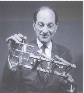
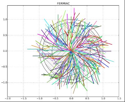
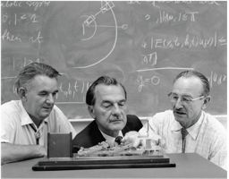
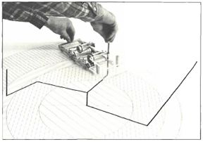
Submitted to ANS Nuclear Technology (2021), LA-UR-21-22202

Figure 7: Portion of Richtmyer's response to von Neumann (1947).

 Richtmyer responded (Figure 7) conveying that he was very interested in the
idea but made some suggested changes to von Neumann’s assumptions. Richtmyer
suggested allowing for multiple fissionable materials, no fission energy-spectrum
dependence, single neutron multiplicity, and to run for computer time and not collisions.
The coding for ENIAC was finalized in December 1947 and contained significant
advances in neutron transport including step-wise continuous-energy neutron cross
section data, fission spectra, and nuclear cross sections tabulated at interval mid-points
with histogram energy-dependence. The first-ever pseudo-random number generator
was also created. The first Monte Carlo calculations were carried out on ENIAC in
April/May 1948.

 III.C. Enrico Fermi and the FERMIAC
 In 1947, when the ENIAC was out of service while being moved to the Ballistics
Research Laboratory, Enrico Fermi invented a 30-cm long, hand-operated, analog,
mechanical computer that was used to trace the histories of neutrons moving through
materials using the Monte Carlo method. The machine, called the FERMIAC, was
constructed by L.D.P. King. King worked at Omega Site in Los Alamos with the Water
Boiler Reactor. Enrico Fermi was a part of the Los Alamos staff during the war and
returned to the University of Chicago postwar but remained a consultant to Los Alamos
and frequently visited. In 1947, he found his fellow scientists frustrated with having a
novel method for solving neutron diffusion (Monte Carlo) and not having an
appropriate computer to use it. ENIAC was being moved from the University of
Pennsylvania to Aberdeen Proving Grounds. During one visit, Fermi discussed creating
a mechanical device to follow neutron tracks through materials with King at a family
picnic. He explained the Monte Carlo process and how the device would work to King.
King spent some time with Fermi in the Omega site workshop to design the mechanical
Monte Carlo computer. The result was a trolley with a 10-step brass roller which would
roll out the neutron range in the given material. The FERMIAC required a scaled
drawing of the nuclear device, physics data tables, and random number lists. After the
initial collection of source neutrons were decided on, a mark on the scaled drawing was
made to note the precise point of collision to determine the next flight path and angle.
Elapsed time was based on the neutron velocity and was grouped as “fast” or “slow”.
Distance traveled between collisions was mechanically measured based on the neutron
velocity and material properties.
 Bengt Carlson’s T-Division Group at Los Alamos used the FERMIAC from
1947 to 1949 to model various nuclear systems with at least 100 source neutrons. An
example of one of its uses was to determine the change in neutron population with time.

Submitted to ANS Nuclear Technology (2021), LA-UR-21-22202

An increasing neutron population would represent a supercritical system and a
decreasing population would represent a subcritical system. A steady neutron
population indicated a critical system. Bengt Carlson said that “although the trolley
itself had become obsolete by 1949, the lessons learned from it were invaluable.”44
 Recently, the Enrico Fermi Center in Italy became interested in the FERMIAC.
Using the original Los Alamos FERMIAC drawings, a replica was built at the Italian
research agency National Institute for Nuclear Physics in 2015. They recreated the
procedure for using the FERMIAC. A simulation using the replica was made for an air-
cooled, uranium graphite reactor. Figure 9 shows the results of the tracks from 100
source neutrons. The three regions are fuel, air, and graphite. Those neutrons that
sample a fission reaction spawn multiple tracks.45

Figure 8. Stan Ulam, Bengt Carlson, Nicholas Metropolis, and L.D.P King with
FERMIAC (1966).46

Figure 9. FERMIAC tracking particles.47

III.D. Programming the First Monte Carlo Calculations on the ENIAC
 The first ENIAC Monte Carlo calculations were chain reaction simulations for
Los Alamos and occurred in three separate groups of problems: April–May 1948,
October–November 1948, and May–June 1949. There were Monte Carlo calculations
run for Argonne for nuclear reactor calculations in December 1948,36 that used the same
basic Monte Carlo algorithm as in the two previous calculations. These ENIAC
calculations were all performed at the Army's Aberdeen Proving Ground in Maryland.
 The Los Alamos model for performing calculations on the ENIAC was a two-
step process of planning and coding.36 The planning was the theoretical development of

Submitted to ANS Nuclear Technology (2021), LA-UR-21-22202

the algorithm to solve the problem being considered. The coding was teaching or
programming the ENIAC how execute the algorithm.
 John Von Neumann did the planning to create the algorithm to solve the neutron
transport problem. Flow diagrams of the algorithm were considered crucial to providing
a rigorous approach for the translation of the mathematical expressions into machine
language programs. Two complete Monte Carlo flow diagrams from 1947 have been
preserved.36

Figure 10. Programming flow chart for Monte Carlo calculation on ENIAC (need
permission to reproduce).36

 Before coding could begin, they and the BRL staff converted ENIAC into a
stored program computer, programming via patch cables would no longer be required.36
 The coding of the Monte Carlo run was performed by both Klara Von Neuman
and Nicholas Metropolis.36 Much of the responsibility for diagramming and coding the
Monte Carlo algorithm belonged to Klara Von Neumann. She described programming
as being “just like a very amusing and rather intricate jigsaw puzzle, with the added
incentive that it was doing something useful.” For 32 days straight in April 1948, they
installed the new control system, checked the code, and ran ENIAC day and night.
Klara was “very run-down after the siege in Aberdeen and had lost 15 pounds.”
Programming and running the ENIAC was not an easy task.36
 Klara von Neumann documented the techniques used to program the Monte
Carlo algorithm in a manuscript “III: Actual Technique—The Use of the ENIAC.”36
This document began with a discussion of the conversion of the ENIAC to support the
new code paradigm, documented the data format used on the punched cards, and
outlined in reasonable detail the overall structure of the computation and the operations
performed at each stage. An expanded and updated version of this report was written by
Klara von Neumann and edited in collaboration with Nick Metropolis and John von

Submitted to ANS Nuclear Technology (2021), LA-UR-21-22202

Neumann during September 1949. It contains a detailed description of the
computations, highlighting the changes in the flow diagram, program code, and manual
procedures between the two versions.36
 The first Monte Carlo problems included “complex geometries and realistic
neutron-velocity spectra that were handled easily.”38 The algorithm used for the ENIAC
is similar in many respects to present-day Monte Carlo neutronics codes: read the
neutron's characteristics, find its velocity, calculate the distance to boundary, calculate
the neutron cross section, determine if the neutron reached time census, determine if the
neutron escaped, refresh the random number, and determine the collision type.36 A card
would be punched at the end of each neutron history and the main loop restarted. The
neutron history punched cards were then subjected to a variety of statistical analyses.38
 The 840-instruction Monte Carlo program on the ENIAC included a number of
firsts for computer programming. “The program included a number of key features of
the modern code paradigm. It was composed of instructions written using a small
number of operation codes, some of which were followed by additional arguments.
Conditional and unconditional jumps were used to transfer control between different
parts of the program. Instructions and data shared a single address space, and loops
were combined with index variables to iterate through values stored in tables. A
subroutine was called from more than one point in the program, with the return address
stored and used to jump back to the appropriate place on completion. This was the first
program ever executed to incorporate these other key features of the modern code
paradigm.”36
 The ENIAC Monte Carlo calculations were extremely successful.36,38 The
unique combination of national security needs, brilliant scientists, the first
programmable computer, and very clever programmers of ENIAC made these results
possible. Today's Monte Carlo codes build on these first ENIAC results.

III.E. Generation and Use of Random Numbers on the ENIAC
 “This meant generating individual neutron histories as dictated by random
mechanisms-a difficult problem in itself,” Metropolis explained. “Thus, neutrons could
have different velocities and could pass through a variety of heterogeneous materials of
any shape or density. Each neutron could be absorbed, cause fission or change its
velocity or direction according to predetermined computed or measured probability. In
essence, the ‘fate’ of a large number of neutrons could be followed in detail from birth
to capture or escape from a given system.”44
 A “Monte Carlo” calculation has been generally defined as one that makes
explicit use of random numbers. Nature is full of completely random processes such as
neutron transport, the number and energy of neutrons emitted from nuclear fission, and
radioactive decay. For example, if a neutron is born in an infinite material with a
specified energy, location, and direction, the neutron will undergo various interactions
at different locations in the material. If a second neutron is born in the material with the
same energy, location, and direction, that neutron will have a different set of
interactions at different locations in the material. Each neutron random walk will be
different. Any attempt to model these neutron random walks must include a capability
to model this random behavior.

III.E.1. Random Numbers for Sampling Random Processes
 The availability of random numbers uniformly distributed in the interval (0,1) is
absolutely essential to obtain correct results when modeling any random process. These

Submitted to ANS Nuclear Technology (2021), LA-UR-21-22202

random numbers will be used to sample a probability density function to select the
outcome of a process or event. In the case of the neutrons above in an infinite material,
random numbers would be used to sample a distance to collision, the isotope that was
collided with, the type of collision that occurred (e.g., scatter, fission, or absorption),
and the energy and direction of the neutron(s) after collision if it is not absorbed.
 Before the advent of electronic digital computers, random numbers were
produced in the form of tables that were used as needed for hand calculations. Entire
books were published containing only random numbers. As easily imagined, this
method of looking up random numbers by hand was very tedious and time consuming.
 When electronic digital computers became available, a different method for
"looking up" random numbers could be used. Deterministic algorithms were devised
that generated a sequence of pseudo-random numbers. The term "pseudo" indicates that
the deterministic algorithm can repeat the sequence and therefore the random numbers
are not truly random: they imitate randomness. In this paper, the term "random number"
means pseudo-random number. Tests for randomness - no observed patterns or
regularities - were developed to assess how random these deterministic sequences
appeared to be.

III.E.2. Random Number Generation and Use by the ENIAC
 When John Von Neumann was developing the neutron diffusion algorithm
(involving random processes) for the ENIAC, he considered the best way to have
random numbers available for use in the algorithm. The amount of memory available on
the ENAIC was small and could not be used to store a table of random numbers. He
realized that having the ENAIC itself create the random numbers during the neutron
diffusion calculation was going to be much faster than reading them from punched
cards. He developed a Random Number Generator (RNG) for the ENIAC that appeared
to generate acceptable random number sequences and was easy to implement. A famous
1949 quote from John Von Neumann is "Anyone who attempts to generate random
numbers by deterministic means is, of course, living in a state of sin." His quote is to
warn users that these (pseudo-)random numbers are not truly random. However, he
definitely favored the use of these random numbers for modeling random processes as
he himself did on the ENIAC.
 John Von Neumann invented the middle-square method RNG in 1946.48 An n-
digit number (n must even) is squared, resulting in a 2n-digit number (lead zeros are
added if necessary, to make the squared number 2n digits). The middle n digits are used
as the random number. The next "refreshed" random number takes the last random
number and squares it. This process is repeated whenever a new random number is
needed. Values of n used on the ENIAC were 8 and 10 during the first Monte Carlo
calculations. There were statistical tests for randomness that were performed by hand on
the first 3000 numbers generated by this scheme. These tests seemed to indicate that the
numbers appeared to be random.36 It turns out that the middle-square RNG is not a good
one because its period is short and it is possible that this RNG can get stuck on zero. It
was adequate, however, for the ENIAC runs that could only calculate a small number of
neutron histories and therefore, only required a small number of random numbers.
 The code for this RNG in the ENIAC program flow diagram was at first
replicated wherever a random number was required. In late 1947, a different
programming paradigm was used where the RNG was its own entity and was entered
from different locations in the Monte Carlo neutron diffusion program. This technique
of reusing code was one of the first calls to a subroutine in computer programming. The

Submitted to ANS Nuclear Technology (2021), LA-UR-21-22202

result of this work was a series of successful Monte Carlo neutron diffusion
calculations.36

IV. MONTE CARLO METHODS IMPROVEMENTS ARE REQUIRED
(1950–PRESENT)
 As the interest in the Monte Carlo method grew after the successful ENIAC
experiences, many organizations began to study and develop new or modified Monte
Carlo methods for their own applications. Today, Monte Carlo methods are used to
solve problems in many disciplines including the physical sciences, biology,
mathematics, engineering, weather forecasting, artificial intelligence, finance, and
cinema. This discussion will focus on the Los Alamos Monte Carlo developments for
neutronics calculations below 20 MeV since the ENIAC calculations.
 Monte Carlo solutions are usually associated with the integral form of the
neutron transport equation, which can be derived from the integro-differential form.49 It
is called the linearized Boltzmann transport equation and is written as:

 1 
 = + , Ω′ , ′ Σ+ + , Ω′ , ′ Σ% − (Ω ∙ ∇ + Σ# ) 
 4 

 This is a balance equation (gains minus losses) where the time-rate of change in
particle flux is equal to the external source, scattering, and multiplication (gains) minus
the leakage and collisions (losses). This equation can be solved directly by Monte Carlo.
Particle history random walks are sampled one at a time from probability density
functions involving measured physical data. Each particle history is an independent
sample and is only dependent on the last collision event. The Monte Carlo results
(tallies) are integrals over all the random walks to produce an average answer for the
desired quantity. Monte Carlo results are confidence intervals formed by applying the
independent- and identically-distributed Central Limit Theorem.50
 Monte Carlo methods have the distinct advantage of being able to sample all the
phase-space variables as continuous functions and not discretized functions. The
disadvantage is that the estimated statistical error in a tally result decreases as 1/sqrt(N),
where N is the number of histories run. To reduce the error by two, N must increase by
four. Variance reduction methods usually must be used to be able to run efficient Monte
Carlo simulations.
 The Monte Carlo algorithm was the method of choice for solving complicated
neutron diffusion problems in the late 1940s because it was a better model of neutron
transport and was fairly easily adapted to the ENIAC. The Monte Carlo principles used
on the ENIAC are the same ones applied today.
 Modern Monte Carlo developments are discussed below in five areas: theory,
RNGs, computational physics, data libraries, and code development. A comprehensive
list of Los Alamos Monte Carlo references covering the past eight decades is available
online.50

IV.A. Los Alamos Developments in Monte Carlo Transport Theory

IV.A.1. General Monte Carlo Theory
 The Atomic Energy Act of 1946 created the Atomic Energy Commission to
succeed the Manhattan Project. In 1953, the United States embarked upon the “Atoms
for Peace” program with the intent of developing nuclear energy for peaceful

Submitted to ANS Nuclear Technology (2021), LA-UR-21-22202

applications such as nuclear power generation. Meanwhile, computers were advancing
rapidly. These factors led to greater interest in the Monte Carlo method. In 1954 the first
comprehensive review of the Monte Carlo method was published by Herman Kahn,51
and the first book was published by Cashwell and Everett in 1959.52
 The first Los Alamos comprehensive document discussing the theoretical and
practical aspects of Monte Carlo development for neutron (and photon) transport was
written in 1957 in a Los Alamos internal report and later published.52 This report
presents in detail all the aspects of a Monte Carlo particle random walk from birth to
death. The concept of particle weight is discussed, as well as several types of variance
reduction methods such as cell importances, forced collisions, and weight, energy, and
time cutoffs. The central limit theorem and the statistical aspects of Monte Carlo
confidence interval results are also reviewed. The principles presented here were
all incorporated into the first Los Alamos general Monte Carlo code, MCS,53 and still
exist today in the present Monte Carlo code Monte Carlo N-Particle® (MCNP®).54 The
appendix52 lists 20 problems that were solved on the MANIAC I, the Los Alamos
computer that was used after the ENIAC, with the Monte Carlo method.
 The next major Los Alamos Monte Carlo review publication was written in
1975 and described many advances in both computational physics and variance
reduction techniques.55 Both fixed source and nuclear criticality keff eigenvalue
problems are discussed. Some of the topics that are included are sampling by rejection,
importance sampling, splitting and Russian roulette, the exponential transform, and
various tally estimators. The Monte Carlo topics discussed in this document are still in
use today in all Monte Carlo radiation transport codes including the MCNP® code.
 Since 1975, there have been many major Los Alamos developments in Monte
Carlo theory, a few of which are mentioned here. The first is the concept of weight
windows for energy-, time-, and space-dependent particle control.56 Several methods
were developed to set the weight windows for a problem including the MCNP® weight
window generator and adjoint deterministic solutions. A second concept is the
DXTRAN sphere that allows Monte Carlo particles to move to small regions of a
problem that are deemed important.57 Upgrades were made to the random number
generator to allow a longer period and a skip-ahead capability that is required for
parallel Monte Carlo calculations.58 A new method to assess the convergence of Monte
Carlo keff eigenvalue calculations was developed, implemented, and tested in the
MCNP® code.59 New statistical procedures were developed to assess the proper
convergence of Monte Carlo results.60 Research into new Monte Carlo methods is an
ongoing activity. Stay tuned.

IV.A.2 Non-Boltzmann Monte Carlo Tallies
 Another new method was created to be able to use variance reduction for non-
Boltzmann tallies such as pulse-height tallies.61 The Monte Carlo solution to the
Boltzmann Neutron Transport Equation calculates average contributions to a tally such
as flux or current over many particle random walks. These tallies are averages of
portions of a random walk where each portion is treated as a separate, independent
contribution to a tally. For example, if a particle enters a cell, collides (losing energy),
and exits the cell, there would be two contributions to a cell tally: one at each energy.
 The Monte Carlo method offers the possibility of calculating other types of
tallies that include correlations of tracks and progeny tracks within one source history.
These correlated tallies are called non-Boltzmann tallies because the Boltzmann
transport equation contains no information about these correlations. Examples of non-
Boltzmann tallies would be coincidence counting and pulse height tallies. A pulse

Submitted to ANS Nuclear Technology (2021), LA-UR-21-22202

height tally is defined as the sum of the energy deposited in a cell from all the
contributions of one source particle. The final tally would not be known until the source
history and all its progeny have been completed. In the one collision example above,
there would now be one contribution for a pulse height tally in the cell instead of two.
 The detail that exists in all the tracks of a Monte Carlo random walk allows
keeping a record of all of these correlations. As expected, it is much more difficult to
sample correlated tallies than uncorrelated tallies, often making efficient non-
Boltzmann calculations extremely difficult. New variance reduction methods that apply
to a collection of tracks were developed at Los Alamos for these non-Boltzmann class
of tallies including deconvolution, corrected single particle, and the supertrack.61 The
deconvolution method was selected to implement into the MCNP® code.62,63 This
algorithm has been fully tested,64,65 so that efficient pulse height tally calculations using
variance reduction can be made.

IV.B. Random Number Generators
 There are many different deterministic RNGs that have been developed over the
decades since Monte Carlo and other statistical sampling methods have become
popular. Before being used, these RNGs are tested for repeatability, robustness,
computational efficiency, and random behavior of the calculated random numbers to
assess their ability to correctly sample random processes.
 The period of a RNG is the number of random numbers that can be generated
before the random number sequence repeats itself. As computers became faster and
calculations became more complex, RNGs with longer periods were required so that no
random numbers are reused during the modeling of the random processes.
 There are two types of RNGs available today: hardware-based RNGs that are
constantly changing based on some environmental variable(s) and are therefore not
repeatable, and the deterministic pseudo RNGs that are repeatable. Pseudo RNGs are
the method of choice for Monte Carlo calculations because they are repeatable and
therefore can be easily tested and calculations more readily compared.
 The pseudo RNGs of today are vastly superior to the middle-square RNG
method of ENIAC times. They are more random, are extremely robust, have much
longer periods, and allow easy access to any location in the sequence. In addition, the
new statistical tests for randomness are more sensitive at finding patterns and
regularities. A detailed discussion of all the RNGs available today is beyond the scope
of this paper. What follows is a brief summary of the RNGs available for use in
neutronics calculations by the Los Alamos Monte Carlo N-Particle® transport code
MCNP®.66
 The big improvement in RNGs was the Linear Congruential Generator (LCG)
that first appeared in 195167 and was later improved in 1958.68 LCGs are the oldest, best
known, and most studied RNGs. Each random number is calculated based on a
recurrence relation involving the previous random number. The initial random number
is called the seed. LCGs have many desirable characteristics for Monte Carlo
calculations.58 They have been extensively studied and tested. They are repeatable, have
long, known periods, are robust, require little computer memory, and are
computationally very efficient. It is easy to skip ahead to any location in the sequence
so that the i_th source particle always starts with the same sequence for the specified
LCG seed. This feature enables correlated sampling comparisons between similar
calculations. This skip-ahead capability is also crucial for performing parallel Monte
Carlo calculations. For these reasons, the LCG is used in many Monte Carlo radiation
transport codes including the MCNP® code.