Machine-learning methods for stream water temperature prediction
←
→
Page content transcription
If your browser does not render page correctly, please read the page content below

Hydrol. Earth Syst. Sci., 25, 2951–2977, 2021
https://doi.org/10.5194/hess-25-2951-2021
© Author(s) 2021. This work is distributed under
the Creative Commons Attribution 4.0 License.

Machine-learning methods for stream water temperature prediction
Moritz Feigl1, , Katharina Lebiedzinski1, , Mathew Herrnegger1 , and Karsten Schulz1
1 Institutefor Hydrology and Water Management, University of Natural Resources and Life Sciences, Vienna, Austria
 These   authors contributed equally to this work.

Correspondence: Moritz Feigl (moritz.feigl@boku.ac.at)

Received: 21 December 2020 – Discussion started: 14 January 2021
Revised: 15 April 2021 – Accepted: 27 April 2021 – Published: 31 May 2021

Abstract. Water temperature in rivers is a crucial environ-       parameter sets for the tested models, showing the importance
mental factor with the ability to alter hydro-ecological as       of hyperparameter optimization. Especially the FNN model
well as socio-economic conditions within a catchment. The         results showed an extremely large RMSE standard deviation
development of modelling concepts for predicting river wa-        of 1.60 ◦ C due to the chosen hyperparameters.
ter temperature is and will be essential for effective inte-         This study evaluates different sets of input variables,
grated water management and the development of adapta-            machine-learning models and training characteristics for
tion strategies to future global changes (e.g. climate change).   daily stream water temperature prediction, acting as a ba-
This study tests the performance of six different machine-        sis for future development of regional multi-catchment wa-
learning models: step-wise linear regression, random forest,      ter temperature prediction models. All preprocessing steps
eXtreme Gradient Boosting (XGBoost), feed-forward neu-            and models are implemented in the open-source R package
ral networks (FNNs), and two types of recurrent neural net-       wateRtemp to provide easy access to these modelling ap-
works (RNNs). All models are applied using different data         proaches and facilitate further research.
inputs for daily water temperature prediction in 10 Austrian
catchments ranging from 200 to 96 000 km2 and exhibiting
a wide range of physiographic characteristics. The evalu-
                                                                  1   Introduction
ated input data sets include combinations of daily means of
air temperature, runoff, precipitation and global radiation.      Water temperature in rivers should not be considered only a
Bayesian optimization is applied to optimize the hyperpa-         physical property, since it is a crucial environmental factor
rameters of all applied machine-learning models. To make          and a substantial key element for water quality and aquatic
the results comparable to previous studies, two widely used       habitats. In particular, it influences riverine species by gov-
benchmark models are applied additionally: linear regression      erning e.g. metabolism (Álvarez and Nicieza, 2005), distri-
and air2stream.                                                   bution (Boisneau et al., 2008), abundance (Wenger et al.,
   With a mean root mean squared error (RMSE) of 0.55 ◦ C,        2011), community composition (Dallas, 2008) and growth
the tested models could significantly improve water temper-       (Imholt et al., 2010); thus, aquatic organisms have a specific
ature prediction compared to linear regression (1.55 ◦ C) and     range of river temperature they are able to tolerate (Caissie,
air2stream (0.98 ◦ C). In general, the results show a very sim-   2006). Due to the impact of water temperature on chemical
ilar performance of the tested machine-learning models, with      processes (Hannah et al., 2008) and other physical properties
a median RMSE difference of 0.08 ◦ C between the models.          such as density, vapour pressure and viscosity (Stevens et al.,
From the six tested machine-learning models both FNNs and         1975), stream temperature indirectly influences key ecosys-
XGBoost performed best in 4 of the 10 catchments. RNNs            tem processes such as primary production, decomposition
are the best-performing models in the largest catchment, in-      and nutrient cycling within rivers (Friberg et al., 2009). These
dicating that RNNs mainly perform well when processes             parameters and processes affect the level of dissolved oxygen
with long-term dependencies are important. Furthermore, a         (Sand-Jensen and Pedersen, 2005) and, of course, have a ma-
wide range of performance was observed for different hyper-       jor influence on water quality (Beaufort et al., 2016).

Published by Copernicus Publications on behalf of the European Geosciences Union.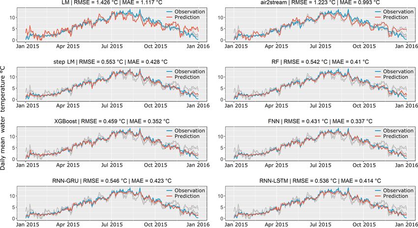
2952                                    M. Feigl et al.: Machine-learning methods for stream water temperature prediction

   Besides its ecological importance, river temperature is also      arguments are also the reasons why data-intensive process-
of socio-economic interest for electric power and industry           based models are widely used despite their high complexity.
(cooling), drinking water production (hygiene, bacterial pol-           Statistical and machine-learning models are grouped into
lution) and fisheries (fish growth, survival and demographic         parametric approaches, including regression (e.g. Mohseni
characteristics) (Hannah and Garner, 2015). Hence, a chang-          and Stefan, 1999) and stochastic models (e.g. Ahmadi-
ing river temperature can strongly alter the hydro-ecological        Nedushan et al., 2007) and non-parametric approaches based
and socio-economic conditions within the river and its neigh-        on computational algorithms like neural networks or k-
bouring region. Assessing alterations of this sensitive vari-        nearest neighbours (Benyahya et al., 2007). In contrast to
able and its drivers is essential for managing impacts and en-       process-based models, statistical models cannot inform about
abling prevention measurements.                                      energy transfer mechanisms within a river (Dugdale et al.,
   Direct temperature measurements are often scarce and              2017). However, unlike process-based models, they do not
rarely available. For successful integrated water manage-            require a large number of input variables, which are unavail-
ment, it will be essential to derive how river temperature will      able in many cases. Non-parametric statistical models have
be developing in the future, in particular when considering          gained attention in the past few years. Especially machine-
relevant global change processes (e.g. climate change), but          learning techniques have been proofed to be useful tools in
also on shorter timescales. The forecast, for example, of river      river temperature modelling already (Zhu and Piotrowski,
temperature with a lead time of a few days can substantially         2020).
improve or even allow the operation of thermal power plants.            For this study we chose a set of state-of-the-art machine-
Two aspects are important: the efficiency of cooling depends         learning models that showed promising results for water tem-
on the actual water temperature. On the other hand, legal con-       perature prediction or in similar time-series prediction tasks.
straints regarding maximum allowed river temperatures due            The six chosen models are step-wise linear regression, ran-
to ecological reasons can be exceeded when warmed-up wa-             dom forest, eXtreme Gradient Boosting (XGBoost), feed-
ter is directed into the river after the power plant. This is es-    forward neural networks (FNNs) and two types of recurrent
pecially relevant during low-flow conditions in hot summers.         neural networks (RNNs). Step-wise linear regression models
Knowledge of the expected water temperature in the next few          combine an iterative variable selection procedure with lin-
days is therefore an advantage. An important step in this con-       ear regression models. The main advantage of step-wise lin-
text is the development of appropriate modelling concepts to         ear regression is the possibility of a variable selection proce-
predict river water temperature to describe thermal regimes          dure that also includes all variable interaction terms, which
and to investigate the thermal development of a river.               is only possible due to the short run times when fitting the
   In the past, various models were developed to investi-            model. The main disadvantages are the linear regression spe-
gate thermal heterogeneity at different temporal and spatial         cific assumptions (e.g. linearity, independence of regressors,
scales, the nature of past availability and likely future trends     normality, homoscedasticity) that might not hold for a given
(Laizé et al., 2014; Webb et al., 2008). In general, water           problem, which consequently could lead to a reduced model
temperature in rivers is modelled by process-based models,           performance. To our knowledge only one previous study by
statistical/machine-learning models or a combination of both         Neumann et al. (2003) already applied this method for pre-
approaches. Process-based models represent physical pro-             dicting daily maximum river water temperature.
cesses controlling river temperature. According to Dugdale              The random forest model (RF) (Breiman, 2001) is an
et al. (2017), these models are based on two key steps: first,       ensemble-learning model that averages the results of multiple
calculating energy fluxes to or from the river and then de-          regression trees. Since they consist of a ensemble of regres-
termining the temperature change in a second step. Calcu-            sion trees that are trained on random subsamples of the data,
lating the energy fluxes means solving the energy balance            RF models are able to model linear and non-linear dependen-
equation for a river reach by considering the heat fluxes at         cies and are robust to outliers. RF models are fast and easy
the air–water and riverbed–water interfaces (Beaufort et al.,        to use, as they do not need extensive hyperparameter tuning
2016). These demanding energy budget components are de-              (Fernández-Delgado et al., 2014). This could also be a disad-
rived either by field measurements or by approximations              vantage as it is also difficult to further improve RF models by
(Caissie and Luce, 2017; Dugdale et al., 2017; Webb and              hyperparameter optimization (Bentéjac et al., 2021). To date,
Zhang, 1997), highlighting the complexity and parametriza-           only one previous study by Heddam et al. (2020) applied RF
tion of this kind of model. Although it is not feasible to           for predicting lake surface temperatures. Zhu et al. (2019d)
monitor these components over long periods or at all points          used bootstrap-aggregated decision trees, which are similar
along a river network and contributing catchments (Johnson           but do not include the random variable sampling for splitting
et al., 2014), they provide clear benefits: (i) give insights into   the tree nodes, which is an important characteristic of the RF
the drivers of river water temperature and (ii) inform about         model.
metrics, which can be used in larger statistical models and             XGBoost (Chen and Guestrin, 2016) is also a regression
(iii) different impact scenarios (Dugdale et al., 2017). These       tree-based ensemble-learning model. However, instead of av-
                                                                     eraging multiple individual trees, XGBoost builds comple-

Hydrol. Earth Syst. Sci., 25, 2951–2977, 2021                                         https://doi.org/10.5194/hess-25-2951-2021
M. Feigl et al.: Machine-learning methods for stream water temperature prediction                                               2953

mentary trees for prediction, which allows for very different       colroaz, 2015). Linear regression models are widely used for
functional relationships compared to random forests. Differ-        river water temperature studies. While earlier studies used
ently from RF models, XGBoost depends on multiple hyper-            mainly air temperature as a regressor to predict river wa-
parameters, which makes it harder and more computationally          ter temperature (e.g. Smith, 1981; Crisp and Howson, 1982;
expensive to apply (Bentéjac et al., 2021). XGBoost showed          Mackey and Berrie, 1991; Stefan and Preud’homme, 1993),
excellent performances in a range of machine-learning com-          more recent publications use a wider range of input variables
petitions (Nielsen, 2016) and also in hydrological time-series      or some modification to the standard linear regression model
applications (e.g. Ni et al., 2020; Gauch et al., 2019; Ibra-       (e.g. Caldwell et al., 2013; Li et al., 2014; Segura et al., 2015;
hem Ahmed Osman et al., 2021), which makes it a promis-             Arismendi et al., 2014; Naresh and Rehana, 2017; Jackson
ing candidate model for this study. To the authors’ knowl-          et al., 2018; Trinh et al., 2019; Piotrowski and Napiorkowski,
edge, XGBoost has not been applied for river water tempera-         2019). air2stream is a hybrid model for predicting river wa-
ture predictions yet. However, results from short-term water        ter temperature, which combines a physically based struc-
quality parameter predictions, which also include water tem-        ture with a stochastic parameter calibration. It was already
perature, show promising performances (Lu and Ma, 2020;             applied in multiple studies over a range of catchments and
Joslyn, 2018).                                                      generally had an improved performance compared to linear
   FNNs (White and Rosenblatt, 1963) are the first and sim-         regression and other machine-learning models (e.g. Piccol-
plest type of neural networks. FNNs have already been               roaz et al., 2016; Yang and Peterson, 2017; Piotrowski and
applied in numerous stream water temperature prediction             Napiorkowski, 2018; Zhu et al., 2019d; Piotrowski and Na-
studies, which range from simple one hidden layer mod-              piorkowski, 2019; Tavares et al., 2020).
els (e.g. Risley et al., 2003; Bélanger et al., 2005; Chenard          Most studies mainly use air temperature and discharge
and Caissie, 2008; McKenna et al., 2010; Hadzima-Nyarko             as inputs for water temperature prediction (e.g. Piccolroaz
et al., 2014; Rabi et al., 2015; Zhu et al., 2018; Temizyurek       et al., 2016; Naresh and Rehana, 2017; Sohrabi et al., 2017),
and Dadaser-Celik, 2018) to multiple hidden-layer models            while others use additional information from precipitation
with a hyperparameter optimization (Sahoo et al., 2009) and         (e.g. Caldwell et al., 2013) and/or solar radiation (e.g. Sa-
to more complex FNN (hybrid) architectures and ensem-               hoo et al., 2009). Additionally, air temperature can either be
bles of FNNs (e.g. DeWeber and Wagner, 2014; Piotrowski             included as mean, maximum or minimum daily temperature
et al., 2015; Abba et al., 2017; Graf et al., 2019; Zhu et al.,     (e.g. Piotrowski et al., 2015). To further investigate which
2019a, b). While FNNs are very flexible and a one-layer FNN         meteorological and hydrological inputs are important and
can theoretically approximate any functions (Pinkus, 1999),         necessary for water temperature prediction, we here use mul-
they are prone to overfitting and dependent on input data scal-     tiple sets of input data and compare their outcome. Especially
ing and an adequate choice of hyperparameters.                      knowing how simple models with few data inputs perform in
   In contrast to FNNs, recurrent neural networks (RNNs)            comparison with more complex input combinations can give
are networks developed specifically to process sequences            insight into how to plan applications of water temperature
of inputs. This is achieved by introducing internal hidden          modelling for a range of purposes.
states allowing one to model long-term dependencies in data            Machine-learning models are generally parameterized by
at the cost of higher computational complexity (Hochreiter          a set of hyperparameters that have to be chosen by the user
and Schmidhuber, 1997) and longer run times. Furthermore,           to maximize performance of the model. The term “hyperpa-
gaps in the observation time series can reduce the number           rameters” refers to any model parameter that is chosen before
of usable data points significantly, as a certain number of         training the model (e.g. neural network structure). Depend-
previous time steps are needed for prediction. While there          ing on the model, hyperparameters can have a large impact
are many different types of RNNs, we focused on the two             on model performance (Claesen and De Moor, 2015) but are
most widely known, the long short-term memory (LSTM)                still most often chosen by rules of thumb (Hinton et al., 2012;
(Hochreiter and Schmidhuber, 1997) and the gated recur-             Hsu et al., 2003) or by testing sets of hyperparameters on a
rent unit (GRU) (Cho et al., 2014). To the authors’ knowl-          predefined grid (Pedregosa et al., 2011). In this study we ap-
edge, RNNs have been used in one study by Stajkowski et al.         ply a hyperparameter optimization using the Bayesian opti-
(2020), in which a LSTM in combination with a genetic al-           mization method (Kushner, 1964; Zhilinskas, 1975; Močkus,
gorithm hyperparameter optimization was used to forecast            1975; Močkus et al., 1978; Močkus, 1989) to minimize the
hourly urban river water temperature. However, LSTMs have           possibility of using unsuitable hyperparameters for the ap-
recently been applied in a wide range of hydrological studies       plied models and to investigate the spread in performance
and showed promising results for time-series prediction tasks       depending on the chosen hyperparameters.
(e.g. Kratzert et al., 2018, 2019; Xiang et al., 2020; Li et al.,      This publication presents a thorough investigation of mod-
2020).                                                              els, input data and model training characteristics for daily
   To make findings comparable with other studies investi-          stream water temperature prediction. It consists of the appli-
gating this approach, we apply two benchmark models as the          cation of six types of machine-learning models on a range
baseline: linear regression and air2stream (Toffolon and Pic-       of different catchments using multiple sets of data inputs.

https://doi.org/10.5194/hess-25-2951-2021                                        Hydrol. Earth Syst. Sci., 25, 2951–2977, 2021
2954                                  M. Feigl et al.: Machine-learning methods for stream water temperature prediction

The present work’s originality includes (i) application of a      fields of several meteorological parameters on a 1×1 km grid
range of ML models for water temperature prediction, (ii) the     in 15–60 min time steps. For the presented study, the 15 min
use of different climatic variables and combinations of these     INCA GL analysis fields were aggregated to daily means.
as model inputs, and (iii) the use of Bayesian optimization       The catchment means of all variables are shown in Table 1.
to objectively estimate hyperparameters of the applied ML         By using high-resolution spatially distributed meteorologi-
models. The resulting performance of all models is compared       cal data as the basis for our inputs, we aim to better represent
to two widely applied benchmark models to make the pre-           the main drivers of water temperature changes in the catch-
sented results comparable. Finally, all methods and models        ments. Similar data sets are available for other parts of the
are incorporated into an open-source R library to make the-       world, e.g. globally (Hersbach et al., 2020), for North Amer-
ses approaches available for researchers and industries.          ica (Thornton et al., 2020; Werner et al., 2019), for Europe
                                                                  (Brinckmann et al., 2016; Razafimaharo et al., 2020) and for
                                                                  China (He et al., 2020).
2     Methods
                                                                  2.2   Data preprocessing
2.1    Study sites and data
                                                                  The applied data preprocessing consists of aggregation of
In Austria there are 210 river water temperature measure-         gridded data, feature engineering (i.e. deriving new features
ment stations available, sometimes with 30+ years of data.        from existing inputs) and splitting the data into multiple sets
This large number of available data in Austria are highly         of input variables. Since river water temperature is largely
advantageous for developing new modelling concepts. Ad-           controlled by processes within the catchment, variables with
ditionally, a wide range of catchments with different phys-       an integral effect on water temperature over the catchment
iographic properties are available, ranging from high-alpine,     (i.e. Ta , Tmax , Tmin , P and GL) are aggregated to catchment
glacier-dominated catchments to lowland rivers, with mean-        means.
dering characteristics.                                              Computing additional features from a given data set (i.e.
   For this study, 10 catchments with a wide range of phys-       feature engineering) and therefore having additional data
iographic characteristics, human impacts (e.g. hydropower,        representation can significantly improve the performance of
river regulation) and available observation period length         machine-learning models (Bengio et al., 2013). Previous
were selected. Including study sites with diverse properties      studies have shown that especially time information is impor-
allows for validation of the applicability and performance        tant for water temperature prediction. This includes time ex-
of the introduced modelling approach. The catchments are          pressed as day of year (e.g. Hadzima-Nyarko et al., 2014; Li
situated in Austria, Switzerland and Germany, with outlets        et al., 2014; Jackson et al., 2018; Zhu et al., 2018, 2019c, d),
located in the Austrian Alps or adjacent flatlands. All catch-    the content of the Gregorian calendar (i.e. year, month, day)
ments and gauging stations are shown in Fig. 1, and their         (Zhu et al., 2019b), or expressed as the declination of the
main characteristics are summarized in Table 1.                   Sun (Piotrowski et al., 2015), which is a function of the day
   The gauging stations are operated by the Austrian Hy-          of the year. Nevertheless, using cyclical features like day of
drographical Service (HZB) and measure discharge (Q) in           the year as an integer variable will most likely reduce model
15 min intervals and water temperature (Tw ) in a range of dif-   performance, since days 1 and 365 are as close together as
ferent time intervals (daily mean – 1 min). The temperature       1 and 2. To translate time information into a more suitable
sensors are situated in a way that complete mixing can be as-     format, we chose to transform months and days of months
sumed, e.g. after a bottom ramp. Consequently, the measured       into trapezoidal fuzzy sets, called fuzzy months. Similar to
water temperature should reflect the water temperature of the     dummy encoding, the values of a fuzzy month are between 0
given cross section.                                              and 1. They are equal to 1 on the 15th of the corresponding
   The meteorological data used in this study are daily mean      month and linearly decreasing each day until they are zero
air temperature (Ta ), daily max air temperature (Tmax ), daily   on the 15th day of the previous and following months. There-
min air temperature (Tmin ), precipitation sum (P ) and global    fore, the values of two adjacent months will be around 0.5 at
radiation (GL). Ta , Tmax , Tmin and P were available from        the turn of the month. By encoding the categorical variable
the SPARTACUS project (Hiebl and Frei, 2016, 2018) on             “month” into these 12 new fuzzy variables, it should be pos-
a 1 × 1 km grid from 1961 onward. The SPARTACUS data              sible to represent time of the year influence more smoothly,
were generated by using observations and external drift krig-     as no jumps in monthly influence are possible. Initial test
ing to create continuous maps. GL data were available from        showed that the advantage of this representation exceeds the
the INCA analysis (Integrated Nowcasting through Compre-          disadvantage of using 12 variables instead of 1 or 2. A simi-
hensive Analysis) (Haiden et al., 2011, 2014) from 2007 on-       lar approach for encoding time variables was already applied
ward. The INCA analysis used numerical weather simula-            by Shank et al. (2008).
tions in combination with observations and topographic in-           Besides time variables, a previous study by Webb et al.
formation to provide meteorological analysis and nowcasting       (2003) showed that lag information is significantly associ-

Hydrol. Earth Syst. Sci., 25, 2951–2977, 2021                                      https://doi.org/10.5194/hess-25-2951-2021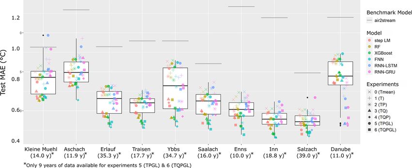
M. Feigl et al.: Machine-learning methods for stream water temperature prediction                                                       2955

Figure 1. Study sites in Austria, Germany and Switzerland. All gauging station IDs refer to the IDs in Table 1. Delineation sources:
Bayrisches Landesamt für Umwelt; HAO: Hydrological Atlas of Austria digHAO (BMLFUW, 2007).

Table 1. Overview of study catchment characteristics, including means of meteorological values of catchment means (Tw , Q, Ta , P , GL),
catchment areas (Area), mean catchment elevations (Elevation), catchment glacier and perpetual snow cover (Glacier), available data time
periods (Time period) and number of years with data (Years). IDs refer to the IDs used in Fig. 1. The percentage of glacier and perpetual snow
cover was computed from the CORINE Land Cover data 2012 and the mean catchment elevation from the EU-DEM v1.1 digital elevation
model with 25 × 25 m resolution.

                                                                  Area    Elevation    Glacier     Tw           Q       Ta     P       GL
  ID   Catchment      Gauging station   Time period   Years      (km2 )   (m NAP)         (%)    (◦ C)     (m3 /s)   (◦ C)   (mm)   (W/m2 )
  1    Kleine Mühl    Obermühl          2002–2015      14.0       200.2          602         0    8.87       3.12     8.71   2.73      135
  2    Aschach        Kropfmühle        2004–2015      11.9       312.2          435         0   10.78       3.80     9.57   2.50      136
  3    Erlauf         Niederndorf       1980–2015      35.3       604.9          661         0    9.42      15.27     7.99   3.59      127
  4    Traisen        Windpassing       1998–2015      17.7       733.3          697         0    9.83      14.88     8.47   3.33      131
  5    Ybbs           Greimpersdorf     1981–2015      34.7     1 116.6          691         0    9.87      31.50     7.97   3.77      127
  6    Saalach        Siezenheim        2000–2015      16.0     1 139.1         1196         0    8.50      39.04     6.72   4.60      135
  7    Enns           Liezen            2006–2015      10.0     2 116.2         1419         0    1.19      67.56     5.62   3.60      137
  8    Inn            Kajetansbrücke    1997–2015      18.8     2 162.0         2244       2.8    6.00      59.26     0.12   2.56      153
  9    Salzach        Salzburg          1977–2015      39.0     4 425.7         1475       1.4    7.63     178.11     5.22   4.16      136
  10   Danube         Kienstock         2005–2015      11.0    95 970.0          827       0.4   10.77   1 798.31    10.05   2.13      131

ated with water temperature and can improve model perfor-                 mean air temperature and fuzzy months are used for predic-
mance. The lag period of 4 d was chosen based on an initial               tions. Experiment 1 (T ) will be able to show the benefit of
data analysis that included (i) assessing partial autocorrela-            including Tmax and Tmin . Experiments 2–4 consist of com-
tion plots of water temperatures, (ii) testing for significance           binations of experiment 1 with precipitation and discharge
of lags in linear regression models, and (iii) checking vari-             data. Experiments 5–6 include combinations with GL and
able importance of lags in a random forest model. Therefore,              therefore include only data of the time period 2007–2015 in
to allow for information of previous days to be used by the               which GL data were available.
models, the lags of all variables for the 4 previous days are
computed and used as additional features.
                                                                          2.3    Benchmark models
   Using these input variables, six experiments with different
sets of inputs considering different levels of data availability
are defined. The variable compositions of all experiments are             Two widely applied models for stream water temperature
shown in Table 2. All features include four lags, and each ex-            prediction are used as a benchmark for all models tested
periment also includes fuzzy months as inputs. Experiment 0               in this study: multiple linear regression (LM) models and
(Tmean ) acts as another simple benchmark in which only daily             air2stream (Toffolon and Piccolroaz, 2015). By including
                                                                          these two models, it will be possible to compare this study’s

https://doi.org/10.5194/hess-25-2951-2021                                                Hydrol. Earth Syst. Sci., 25, 2951–2977, 2021
2956 M. Feigl et al.: Machine-learning methods for stream water temperature prediction
Table 2. Overview of available meteorological and hydrological physically based structure with a stochastic parameter cal-
variables and the composition of the different input data set exper- ibration. It was already applied in multiple studies over a
iments. If an input variable is used in a data set, the lags for the 4 range of catchments and generally had an improved perfor-
previous days are included as well. Additionally to the shown vari- mance compared to linear regression models (e.g. Piccolroaz
ables, all experiments use fuzzy months as input. et al., 2016; Yang and Peterson, 2017; Piotrowski and Na-
piorkowski, 2018; Zhu et al., 2019d; Piotrowski and Napi-
Experiment Ta Tmax Tmin P Q GL orkowski, 2019; Tavares et al., 2020). air2stream uses the
0 (Tmean ) X inputs Ta and Q and was derived from simplified physical
1 (T ) X X X relationships expressed as ordinary differential equations for
2 (TP) X X X X heat-budged processes. Due to this simplification, it may be
3 (TQ) X X X X applied like a data-driven model, which depends on parame-
4 (TQP) X X X X X ter calibration. The eight-parameter version of air2stream is
5 (TPGL) X X X X X defined as
6 (TQPGL) X X X X X X
dTw 1
= a [a1 + a2 Ta − a3 Tw
dt θ 4
results to a wider range of previous studies, which investi- t
+ θ a5 + a6 cos 2π − a7 − a8 Tw ], (4)
gated models for stream water temperature prediction. ty
2.3.1 Linear regression where t is the time in days, ty is the number of days per year,
Q̄ is the mean discharge, θ = Q/Q̄ is the dimensionless dis-
Linear regression models are widely used for river water tem- charge and a1,...,8 are the model parameters. This differen-
perature studies. Earlier studies used mainly air temperature tial equation is numerically integrated at each time step using
as a regressor to predict river water temperature (e.g. Smith, the Crank–Nicolson numerical scheme (Crank and Nicolson,
1981; Crisp and Howson, 1982; Mackey and Berrie, 1991; 1947) and the model parameters are calibrated using particle
Stefan and Preud’homme, 1993). More recent publications swarm optimization (Kennedy and Eberhart, 1995).
use a wider range of input variables or some modification
to the standard linear regression model (e.g. Caldwell et al., 2.4 Machine-learning models
2013; Li et al., 2014; Segura et al., 2015; Arismendi et al.,
2014; Naresh and Rehana, 2017; Jackson et al., 2018; Trinh In this study we compare six different machine-learning
et al., 2019; Piotrowski and Napiorkowski, 2019). models: step-wise linear regression (step-LM), RF, XG-
The ordinary least-square linear regression model is de- Boost, FNNs and two RNNs – the long short-term network
fined as (RNN-LSTM) and the gated recurrent unit (RNN-GRU). An
overview and simple depiction of the models are shown in
Y = βX + , (1) Fig. 2.
where Y denotes the vector of the dependent variable (river 2.4.1 Step-wise linear regression
water temperature), X denotes the matrix of independent
variables (e.g. daily mean air temperature, global radiation), Step-wise linear regression models combine an iterative vari-
β denotes the vector of model coefficients and denotes the able selection procedure with linear regression models. The
error term. is assumed to be normal distributed with a di- step-wise variable selection starts at an initial model (e.g. all
agonal covariance matrix. The estimates for the model coef- variables) and removes or adds at each iteration based on a
ficients and the dependent variable, which minimize the sum prespecified criterion. We applied the step-wise variable se-
of squared errors, are given by lection starting with an initial model including all variables
and using the Akaike information criterion (AIC) (Akaike H,
Ŷ = β̂X, (2) 1973). The AIC for a linear regression model is given by
0 −1 0
β̂ = (X X) X Y, (3) Pn 2
!
i=1 (Y i − Ŷ i )
AIC = n × ln + 2k, (5)
where Ŷ and β̂ represent estimated values. The linear regres- n
sion model applied in this study includes an intercept and the
variables Ta and Q as independent variables to predict Tw . where n is the number of samples, ln() the natural logarithm,
Y and Ŷ the observed and predicted water temperatures and
2.3.2 air2stream k the number of selected input variables. The step-wise vari-
able selection is iteratively applied until AIC is at a mini-
air2stream (Toffolon and Piccolroaz, 2015) is a hybrid model mum. Additionally to the variables given in Sect. 2.2, inter-
for predicting river water temperature, which combines a action terms between Ta , Q, GL and P are included.
Hydrol. Earth Syst. Sci., 25, 2951–2977, 2021 https://doi.org/10.5194/hess-25-2951-2021M. Feigl et al.: Machine-learning methods for stream water temperature prediction 2957
Figure 2. Overview of the applied models with Ŷ denoting estimated water temperatures and X the matrix of observed variables. Ŷ1,...,M
are the predictions from individual RF trees. h1, ...,M are the predicted residuals from individual XGBoost trees. f (X, θ) denotes a mapping
from a FNN with the parameters θ . For a given time step, ht denotes the hidden internal state of a RNN cell, ct the internal cell state of a
LSTM cell and f (ht , θ) the mapping from a RNN with the parameters θ. RNNs consist of a cascade of cells, each feeding their internal
states into the next cell, finally resulting in a single feed-forward layer estimating Ŷ from ht .
2.4.2 Random forest 2.4.3 XGBoost
The RF model (Breiman, 2001) is an ensemble-learning XGBoost (Chen and Guestrin, 2016) is a tree-boosting algo-
model based on the idea of bagging (bootstrap aggregating) rithm that was developed based on the already existing con-
(Breiman, 1996). Bagging predictors average multiple model cept of boosting, which was further enhanced to increase ef-
predictions, where each model is trained on a bootstrapped ficiency, scalability and reduced overfitting. Similarly to bag-
sample instead of the full observed sample. This randomness ging, boosting methods combine the prediction of an ensem-
introduced by bootstrapping increases the model’s ability to ble of weak learners to improve prediction accuracy. How-
generalize and to produce stable prediction results. ever, while bagging ensemble members are trained in par-
RF models are bagging predictors which use classification allel, boosting iteratively trains new ensemble members and
and regression trees (CARTs) as a base learner. RF CARTs adds them to the existing ensemble. Boosting was first in-
recursively apply binary splits to the data to minimize en- troduced by Schapire (1990) and then widely applied af-
tropy in the tree nodes. This is done until each node reaches ter the introduction of the Adaboost algorithm (Freund and
a minimum node size or a previously defined maximum tree Schapire, 1995). Friedman (2001) further enhanced boost-
depth is reached. Breiman (2001) showed that adding further ing by adding gradient decent optimization for the boosting
randomness to the bagging method improves prediction ac- iterations. This resulted in the development of gradient tree
curacy. In random forests this is achieved by only selecting boosting (Friedman, 2002), which uses CART as weak learn-
a random subset of available variables for the split at each ers.
node. The estimate for the dependent variable is given by XGBoost is an implementation of gradient tree boosting
with further enhancements in the form of added stochasticity
M
1 X and regularization. The XGBoost estimated for the indepen-
Ŷ = fi (X), (6) dent variable is given by
M m=1
M
where fm denotes a single fitted CART, M the number of Ŷ = 0.5 +
X
ηfm (X), (7)
used CARTs, X the matrix of regressors and Ŷ the vector m=1
of estimated water temperature. A simplified depiction of the
RF algorithm is shown in Fig. 2. RF has two important hyper- where f1 , . . . fM is a sequence of CARTs, η ∈ [0, 1] is the
parameters: the number of predictors sampled at each node learning rate, M is the number of used CARTs, X is the ma-
(mtry) and the minimum size of nodes (min node size). The trix of input features and Ŷ is the vector of estimated water
number of trees was chosen to be constant with 500 trees. temperatures. The mth tree is trained to predict the residu-
https://doi.org/10.5194/hess-25-2951-2021 Hydrol. Earth Syst. Sci., 25, 2951–2977, 20212958 M. Feigl et al.: Machine-learning methods for stream water temperature prediction
als of a model of the form given in Eq. (7), which uses the 2.4.5 Recurrent neural networks
previous m − 1 CARTs. The loss function used to train each
tree includes a regularization term to prevent overfitting. Ad- In contrast to FNNs, RNNs are able to process sequences of
ditionally, overfitting is reduced by only allowing a random inputs. This is achieved by having internal (hidden) states.
subset of samples and variables to be used for constructing While there are many different types of RNNs, we focused
trees and tree nodes at each iteration. A simplified depiction on the two most widely known, the long short-term mem-
of the XGBoost algorithm is shown in Fig. 2. ory (LSTM) (Hochreiter and Schmidhuber, 1997) and the
XGBoost has multiple important hyperparameters that gated recurrent unit (GRU) (Cho et al., 2014). Each layer
have to be chosen before fitting the model: the maximum of an RNN consists of a sequence of cells that share a com-
number of iterations (nrounds), the learning rate (η), the mon set of weights. The cells of both LSTM and GRU are
maximum depth of a tree (max depth), the minimum sum of shown in Fig. 2 and are described in Appendices A1 and A2.
instance weight needed in a child (min node size), the ratio A single RNN cell consists of multiple gates, which refers to
of random subsamples used for growing a tree (subsample) the nodes of a cell where non-linear transformations are ap-
and the random fraction of variables used for growing a tree plied to the inputs and states. The main difference between
(colsample bytree). LSTM and GRU cells is their number of gates and internal
states, where LSTMs are more complex (two internal states
2.4.4 Feed-forward neural networks and three gates) than GRUs (one internal state and two gates).
While in some cases GRUs outperform LSTMs, there is no
FNNs (White and Rosenblatt, 1963) are the first and simplest clear rule of when to use one or the other (Yazidi et al., 2020).
type of neural networks. FNNs consist of multiple layers of Each RNN contains a FNN layer with a single node at its
nodes, where each node is connected to all nodes of the pre- end, which is used to compute the predicted values from the
vious and following layers. A node applies linear and non- hidden states of the last time step (hT ). Both types of RNNs
linear (activation) functions to its input to produce an output. have the same set of hyperparameters that need to be speci-
The general structure of a FNN is shown in Fig. 2. fied before training the model: the number of used RNN lay-
Piotrowski et al. (2020) showed that adding dropout (Hin- ers, the number of units per layer, the numbers of time steps,
ton et al., 2012; Srivastava et al., 2014; Baldi and Sadowski, the dropout ratio, and the batch size.
2014) to FNNs for stream water temperature prediction im- Due to their internal states and the usage of multiple time
proved performance of single-layer FNNs. Dropout refers to steps for prediction, it can be assumed that RNNs do not need
randomly dropping nodes from a layer during training, which time information (here in the form of fuzzy months) for pre-
can prevent overfitting and potentially improve generaliza- dicting water temperature data. To test this assumption, both
tion. We added a dropout to every FNN layer and defined RNN variants are also trained without fuzzy months to check
the dropout rate as a hyperparameter, which can be zero and the influence of these additional variables on model perfor-
therefore also allow for model structures without dropout. mance. Being able to achieve equally good results without
While the parameters (θ ) of the linear function get opti- fuzzy months would reduce training time considerably due
mized using backpropagation (Rumelhart et al., 1986), FNNs to decreasing the input data by 12 dimensions (columns).
have multiple hyperparameters that need to be predefined be-
fore training. These hyperparameters include the activation 2.5 Bayesian hyperparameter optimization
functions, the number of layers, the number of nodes per
layer and the dropout ratio. After initial tests, in which a large Choosing adequate hyperparameters for a machine-learning
set of different activation functions was applied, we chose model can have a large impact on its performance. There-
the scaled exponential linear unit (SELU) activation function fore, it is necessary to apply some sort of optimization pro-
(Klambauer et al., 2017) for all nodes in the network. SELU cedure. While it might be possible to apply a grid search
includes a normalization, which enhances convergence and over the range of all possible parameter value combinations
avoids both vanishing and exploding gradients during back- for a small set of hyperparameters, it is usually not feasible
propagation. The other hyperparameters are optimized as de- due to available computational resources. For that reason, we
scribed in Sect. 2.5. chose to optimize the hyperparameters of nearly all machine-
The hyperparameter optimization approach presented here learning models in this study with the Bayesian optimization
differs from previous studies, which generally assume a set method. Only random forest with three hyperparameters is
of a fixed number of layers and/or nodes per layer that were optimized using a grid search. Step-wise linear regression
derived by a trial-and-error approach (e.g. Bélanger et al., does not have hyperparameters that need optimization.
2005; Hadzima-Nyarko et al., 2014; Piotrowski et al., 2015; Bayesian optimization is a global optimization method
Zhu et al., 2018, 2019d). for blackbox functions (i.e. lacks known structure and is
derivative-free) that is often applied in cases where the ob-
jective function is computationally expensive to evaluate. It
originates from work by Kushner (1964), Zhilinskas (1975),
Hydrol. Earth Syst. Sci., 25, 2951–2977, 2021 https://doi.org/10.5194/hess-25-2951-2021M. Feigl et al.: Machine-learning methods for stream water temperature prediction 2959
Močkus (1975), Močkus et al. (1978), and Močkus (1989) The time-series CV started with an initial window of 730 d
and was later popularized by Jones et al. (1998). It be- for training the following 90 d for validation. The training
came especially well known for being suitable for optimizing set is increased by 90 d at each different cross-validation set
machine-learning hyperparameters after a study by Snoek until the full time series except for the last 90 d was used.
et al. (2012). Therefore, instead of 10 folds, the number of folds for the
Bayesian optimization consists of two parts: a method for time-series CV depends on the time-series length.
statistical inference and an acquisition function for deciding Due to computational and time constraints, hyperparam-
the next sample point. The method for statistical inference is eter optimization for all neural networks was done by us-
usually a Gaussian process (GP) which provides an estimated ing a training/validation split with 60 % data for training and
posterior distribution at each iteration that is an estimate for 20 % data for validation. This allows model validation per-
the function that should be optimized. The acquisition func- formance estimation by training a model once, while a 5
tion is used to find the next point to evaluate during each times repeated 10-fold CV would require training a model 50
optimization step and was chosen to be the upper confidence times. Furthermore, the training/validation split is the stan-
bound (UCB) (Srinivas et al., 2009) in this study. In sum- dard way of training neural networks for real-world applica-
mary, Bayesian optimization constructs a surrogate model at tions.
each iteration during optimization to choose a suitable next Bayesian hyperparameter optimization consists of 20 ran-
point. The hyperparameters of all optimized models and their dom parameter samples and 40 iterations of optimization.
chosen bounds are given in Appendix A3. The data inputs for all neural networks were standardized by
subtracting the mean and dividing by the standard deviation
2.6 Evaluation metrics of the training data. The optimized neural network hyper-
parameter sets are used to create five independently trained
The objective function for all models and the hyperparameter models, from which an ensemble for prediction is created by
optimization is the mean squared error (MSE): taking the average of all five prediction results. Using ensem-
n bles of networks is a way to significantly increase a neural
1X
MSE = (yi − yˆi )2 , (8) network’s ability to generalize and is an often-applied ap-
n i=1 proach which was first introduced by the work of Hansen
and Salamon (1990). In addition, early stopping with pa-
where n is the number of samples (d) and yi the observed tience = 5 was applied to all neural networks to avoid over-
and ŷi the predicted water temperatures. To compare the per- fitting.
formance of different models, the root mean squared error The best-performing model for each model type and ex-
RMSE and the mean absolute error MAE are used: periment is chosen using the validation RMSE. Test RMSE
√ and MAE results are only compared after choosing the mod-
RMSE = MSE, (9) els with minimum validation RMSE. Consequently, it might
n
1X be possible that some models have a superior test perfor-
MAE = |yi − yˆi |. (10) mance but are not chosen as the best-performing model for
n i=1
a specific model type and/or experiment. This should reflect
2.7 Experimental setup a real-world application, where test data act as a previously
unknown future time series.
To be able to objectively compare all applied models, the Table 3 gives an overview of all time periods and the hy-
available data sets are split into two parts: the first 80 % of perparameter optimization details. All models are trained us-
the time series were used for training/validation and the last ing the training/validation period data and either applied CV
20 % were used for testing. We deliberately did not choose or a training/validation split. Models with hyperparameters
a random split, because predicting water temperatures for a are trained multiple times during hyperparameter optimiza-
future time period is a more adequate test for models. This tion. The fully trained models are then applied in the test
is especially relevant for water temperature, which is charac- time period to produce comparable out-of-sample results.
terized by non-stationarity due to climate change (Van Vliet The eight air2stream hyperparameters are optimized using
et al., 2013). The training/validation and test time series are the particle swarm optimization with 500 iterations, 500 par-
compared to assess the difference of water temperature dis- ticles, cognitive and social learning factors set to 2 and inertia
tribution of all catchments. max and min set to 0.9 and 0.4. All models were run on the
The step-wise linear regression model, RF and XGBoost Vienna Scientific Cluster, where each run had access to two
are optimized using cross-validation (CV). Two kinds of CV Intel Xeon E5-2650v2, 2.6 GHz, eight-core CPUs and 65 GB
are applied: a five times repeated 10-fold CV and a time- RAM.
series CV. While the 10-fold CV splits the data randomly, the
time-series CV gradually adds data to an initial part of the
time series while evaluating the performance of each step.
https://doi.org/10.5194/hess-25-2951-2021 Hydrol. Earth Syst. Sci., 25, 2951–2977, 20212960 M. Feigl et al.: Machine-learning methods for stream water temperature prediction
Table 3. Overview of the different modelling time periods and hyperparameter optimization details, including information about cross-
validation (CV), the number of hyperparameters (Hyperparameters) and the number of iterations of the Bayesian hyperparameter optimiza-
tion (Iterations).
Catchment Training/validation period Test period Model CV Hyperparameters Iterations
Kleine Mühl 2002–2012 2013–2015 LM no 0 0
Aschach 2004–2012 2013–2015 air2stream no 8 500
Erlauf 1980–2007 2008–2015 step-LM yes 0 0
Traisen 1998–2011 2012–2015 RF yes 2 60
Ybbs 1981–2007 2008–2015 XGBoost yes 6 60
Saalach 2000–2011 2012–2015 FNN no 4 60
Enns 2006–2013 2014–2015 RNN-GRU no 5 60
Inn 1997–2011 2012–2015 RNN-LSTM no 5 60
Salzach 1977–2007 2008–2015
Danube 2005–2012 2013–2015
2.8 Statistical tests the overall data, the exact length of these time series is de-
pendent on the catchment but is always a subset of the years
The Kruskal–Wallis test (Kruskal and Wallis, 1952) was used 2008–2015. We can observe an increase of 138 % of the me-
to test for differences in overall model performances, differ- dian number of days with water temperature above the 90 %
ent training/model characteristics and different data inputs. quantile between training/validation and test time period in
Dunn’s test for multiple comparison (Dunn, 1964) was used all catchments. This increase ranges from 69 % or from 32 to
for pair-wise comparisons between model performances. To 54 d, in the Danube catchment and up to 285 %, or from 26
investigate the association of model types, experiments and to 100 d, in the Salzach catchment. This change is even more
catchments with test RMSE, an ordinary least-square linear pronounced when comparing the last year of test data (2015)
regression model was used. Level of significance was set to to all other available years, where the median number of days
p = 0.05 for all statistical tests. with water temperatures above the 90 % quantile (computed
for the overall time series) of all catchments increases by
2.9 Open-source R package 273 %. Figure 3 shows the corresponding boxplots of days
with stream temperature above the 90 % quantile for each
All preprocessing steps and models were implemented in catchment in training/validation and in test time period. A
the open-source R package wateRtemp, which is available similar pattern can be observed in the changes in mean yearly
under https://www.github.com/MoritzFeigl/wateRtemp (last stream temperatures. The median increase in mean yearly
access: 25 April 2021) or from Feigl (2021a). This provides water temperature of all catchments is 0.48 ◦ C when com-
easily applicable modelling tools for the water temperature paring training/validation with test time period and 0.77 ◦ C
community and allows all results of this study to be repli- when comparing the last year of the test period (2015) with
cated. All programming was done in R (R Core Team, 2020), all other years. Since the test period is, as shown here re-
where the model development relied heavily on Caret (Kuhn, garding extremes, different from the training/validation pe-
2020), xgboost (Chen et al., 2020) and TensorFlow (Allaire riod, the models are also, at least to some extent, tested on
and Tang, 2020) and the visualizations on ggplot2 (Wickham, how they perform under instationary conditions. This is a
2016). test where environmental models often fail (e.g. Kling et al.,
2015).
3 Results
3.2 Overall performance comparison
3.1 Time period characteristics
Table 4 gives an overview of the best-applied machine-
Due to climate change, both air temperatures and water tem- learning models and the two benchmark models LM and
peratures are steadily increasing (Mohseni and Stefan, 1999; air2stream. This table compares the RMSE and MAE per-
Pedersen and Sand-Jensen, 2007; Harvey et al., 2011; Kȩdra, formances of all models; additional performance metrics are
2020). This is clearly visible when comparing the change shown in Table A1. The mean test RMSE of LM is 1.55 ◦ C
in number of extreme warm days and the increase in mean with an overall range of [1.25, 2.15] ◦ C, while air2stream has
water temperature in all studied catchments with time. For a mean test RMSE of 0.98 ◦ C with an overall range of [0.74,
this we compared the training/validation and test time data 1.17] ◦ C. The performance results for each catchment show
in each catchment. Since test data consist of the last 20 % of that air2stream always outperformed LM and consequently
Hydrol. Earth Syst. Sci., 25, 2951–2977, 2021 https://doi.org/10.5194/hess-25-2951-2021M. Feigl et al.: Machine-learning methods for stream water temperature prediction 2961
Figure 3. Boxplots showing the distribution of numbers of days with stream temperatures above the 90 % quantile per year for all study
catchments for the training/validation and the test time period, where the test time period consists of the last 20 % of data in each catchment.
The 90 % quantile values were estimated using the full time series for each catchment.
results in a significant lower test RMSE (p < 0.001). The additional input parameter, the median performance does not
mean test RMSE of the best machine-learning models per increase further. This could be explained by a reduced time-
catchment is 0.55 ◦ C with an overall range of [0.42, 0.82] ◦ C series length of experiments 5 (TPGL) and 6 (TQPGL), since
and always outperformed the air2stream benchmark. Based global radiation was only available from 2007 on. A com-
on the RMSE means, the highest performing ML model parison between experiments with equal time-series lengths
is 64 % and 43 % better, compared to LM and air2stream. (experiments 0–4 and experiments 5–6) also indicates that
This results in a significantly lower test RMSE of the tested runoff information improves the modelling performance.
machine-learning models compared to the air2stream bench- Figure 4c illustrates the RMSE performance results for
mark (p < 0.001). each catchment shown as boxplots. A corresponding figure
Both XGBoost and FNN were found to be the best- of the MAE results is shown in Fig. A1. The boxplots are
performing model in 4 of 10 analysed catchments each. RF overlayed with scatter-plot points adding an overview of the
was the best-performing model in the Salzach catchment individual performance of each model and experiment com-
and RNN-LSTM in the Danube catchment. Step-LM and bination. To account for a better visibility, the scatter-plot
RNN-GRU did not outperform the other models in any of points are shifted in horizontal direction randomly. The dif-
the study catchments. Experiment 3, which only includes air ference in performance between catchments is clearly visible
temperature and discharge input features, resulted in the best- and ranges from a median RMSE of around 0.93 ◦ C in catch-
performing model in four catchments. Experiment 6, which ments Kleine Mühl and Aschach down to a median RMSE
included all available input features, also produced the best- of 0.58 ◦ C in the Inn catchment.
performing model in four catchments. Experiment 4, which Figure 4c also includes the air2stream benchmark per-
includes air temperature, discharge and precipitation input formance shown as a grey line for each catchment. Nearly
features, performed best in two catchments. all tested experiments and model combinations showed im-
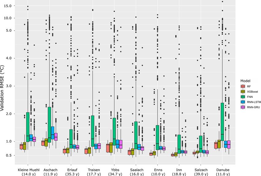
Figure 4 shows the results of all models, catchments and proved performance compared to the air2stream benchmark.
experiment combinations. The boxplots in Fig. 4a show the Only in five catchments could we observe models in combi-
range of model performances depending on the model type. nation with experiments 0, 1, and 5 and one time with exper-
Kruskal–Wallis test results show no significant difference iment 6 that predicted worse than air2stream. There are sur-
(p = 0.11) of the test RMSE of different model types. Fig- prisingly few models considering the fact that experiments 0,
ure 4b shows boxplots of model performance for all experi- 1, 5 and 6 are heavily constrained due to the amount of infor-
ments. Kruskal–Wallis test results show a highly significant mation that is available for prediction. Experiments 0 and 1,
difference of test RMSE of the different experiments (p < which only use air temperature, are still able to improve pre-
10−14 ). The results in Fig. 4b show an increase in median dictions compared to air2stream for all model types in seven
performance with an increasing number of input features un- catchments. Similarly, experiments 5 and 6 with only 6 years
til experiment 4 (TQP). When adding global radiation as an
https://doi.org/10.5194/hess-25-2951-2021 Hydrol. Earth Syst. Sci., 25, 2951–2977, 20212962 M. Feigl et al.: Machine-learning methods for stream water temperature prediction
Table 4. Overview of model performance of the best machine-learning model for each catchment and the two reference models. The best-
performing model results in each catchment are shown in bold font. The best machine-learning model for each catchment was chosen by
comparing validation RMSE values, while test RMSE and test MAE values were never part of any selection or training procedure. The shown
values all refer to the test time period.
Best ML model results LM air2stream
Catchment Model Experiment RMSE (◦ C) MAE (◦ C) RMSE (◦ C) MAE (◦ C RMSE (◦ C) MAE (◦ C)
Kleine Mühl XGBoost 4 (TQP) 0.740 0.578 1.744 1.377 0.908 0.714
Aschach XGBoost 6 (TQPGL) 0.815 0.675 1.777 1.408 1.147 0.882
Erlauf XGBoost 6 (TQPGL) 0.530 0.419 1.354 1.057 0.911 0.726
Traisen FNN 3 (TQ) 0.526 0.392 1.254 0.970 0.948 0.747
Ybbs RF 3 (TQ) 0.576 0.454 1.787 1.415 0.948 0.756
Saalach XGBoost 6 (TQPGL) 0.527 0.420 1.297 1.062 0.802 0.646
Enns FNN 6 (TQPGL) 0.454 0.347 1.425 1.166 1.168 0.671
Inn FNN 3 (TQ) 0.422 0.329 1.376 0.098 1.097 0.949
Salzach FNN 4 (TQP) 0.430 0.338 1.327 1.077 0.743 0.595
Danube RNN-LSTM 3 (TQ) 0.521 0.415 2.145 1.721 1.099 0.910
Mean: 0.554 0.437 1.549 1.235 0.977 0.760
of training data are able to improve predictions compared to ference between the tested machine-learning model RMSE
air2stream for all model types in five catchments. and the air2stream RMSE is −0.39 ◦ C.
From the results in Fig. 4a, b, c it seems likely that per- The relationship between mean catchment elevation,
formance is in general influenced by the combination of glacier fraction and test RMSE was analysed with a linear
model, data inputs (experiment) and catchment, while the model using mean catchment elevation, glacier fraction in
influence of different experiments and catchments is larger percentage of the total catchment area, total catchment area
than the influence of model types on test RMSE. The lin- and the experiments as independent variables and test RMSE
ear regression model for test RMSE with catchment, exper- as the dependent variable. This resulted in a significant asso-
iment and model type as regressors is able to explain most ciation of elevation (p value < 2 × 10⁻¹⁶ ) with lower RMSE
of the test RMSE variance with a coefficient of determina- values and catchment area (p value = 3.91×10⁻⁴ ) and a sig-
tion of R 2 = 0.988. Furthermore, it resulted in significant nificant association of glacier cover (p value = 9.79 × 10⁻⁵ )
association of all catchments (p < 10−15 ), all experiments with higher RMSE values. Applying the same model without
(p < 0.005) and the FNN model type (p < 0.001). The es- using the data of the largest catchment, the Danube, resulted
timated coefficient of the FNN is −0.05, giving evidence of in a significant (p value = 2.12×10⁻¹¹ ) association between
a prediction improvement when applying the FNN model. catchment area and lower RMSE values, while the direction
All other model types do not show a significant association. of the other associations stayed the same.
However, this might be due to a lack of statistical power, as The run times for all applied ML models are summarized
the estimated coefficients of the model types (mean: −0.01, in Table 5. FNN and RF have the lowest median run times
range: [−0.05, 0.02]) are generally small compared to catch- with comparatively narrow inter-quartile ranges (IQRs), so
ment coefficients (mean: 0.86, range: [0.69, 1.06]) and ex- that most models take between 30 min and 1 h to train. XG-
periment coefficients (mean: −0.12, range: [−0.2, −0.04]). Boost has a median run time of around 3 h (172.9 min) and
Overall, the influence of the catchment is higher than the also a comparatively low IQR with a span of 50 min. Step LM
influence of model type and experiment, which is clearly and both RNNs need much longer to train, with median run
shown with their around 1 order of magnitude larger coef- times of around 700 min. They also have a much larger vari-
ficients. ability in the needed run time, especially the step-LM model
Multiple experiments often result in very similar RMSE with an IQR of more than 1500 min. In contrast, the run time
values for a single model type. Furthermore, the best- of the LM model is negligibly small (< 1 s), and air2stream
performing experiments of different model types are always is also considerably faster, with run times of < 2 min in all
very close in performance. This results in a median test catchments.
RMSE difference of the best experiments of different model
types of 0.08 ◦ C and a median test RMSE difference of the 3.3 Detailed analysis for a single catchment
best-performing model and the second best model of another
model type of 0.035 ◦ C. On the other hand, the median dif-
To further investigate the difference in performance, the pre-
diction results for the last year of the test data (2015) of
Hydrol. Earth Syst. Sci., 25, 2951–2977, 2021 https://doi.org/10.5194/hess-25-2951-2021You can also read