New York City Taxis: Demand and Revenue in an Uber World
←
→
Page content transcription
If your browser does not render page correctly, please read the page content below
New York City Taxis: Demand and Revenue in an Uber
                       World
                         Kristin Mammen∗                Hyoung Suk Shim†
                                        December 31, 2017

                                    Rewriting in progress
                                               Abstract
            We empirically examine the effect of Uber presence on (medallion) taxi trip demand
        in NYC. We estimate Uber elasticities of demand for the Yellow cab and Green cab using
        NYC medallion taxi trip records and Uber pick-up records from April to September
        2014, and January to June 2015. The elasticities are estimated along with instrumental
        variable estimations of a taxi trip demand model. We find an empirical evidence that, in
        overall, Uber is a complement, rather than a substitute, for both Yellow cab and Green
        cab passengers. For Yellow cab. the positive and significant elasticity is estimated
        only in Manhattan below 110th street, where 91% of daily Yellow cab trip and 72%
        of daily Uber trip were occurred. In addition, we find different elasticity estimate in
        different time and day at different area. Negative Uber elasticity of Yellow cab estimate
        in Manhattan below 110th street during the morning rush hour implies that; Uber turn
        out to be a substitute during the morning rush hour in the central business district of
        Manhattan.

1       Introduction
Uber is one of leading smartphone app based ride-hailing companies. Its positive effect
that Uber is an efficient taxi service, and it benefits to both passengers and drivers have
recently been examined by [Cramer and Krueger (2016); Hall and Krueger (2016); Cohen
et al. (2016); Chen et al. (2017)]. In the meantime, Uber has been experienced temporary
ban from major cities such as London, Delhi in India, and Austin Texas. Passenger safety,
    ∗
    School of Business, CUNY College of Staten Island, New York, email: Kristin.Mammen@csi.cuny.edu.
    †
    School of Business, CUNY College of Staten Island, New York, email: Hyoungsuk.Shim@csi.cuny.edu.
This research was supported, in part, under National Science Foundation Grants CNS-0958379 and CNS-
0855217 and the City University of New York High Performance Computing Center at the College of Staten
Island.

                                                   1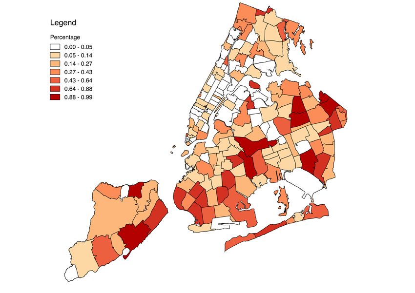
causing congesting, and surge pricing are known issues that Uber has been criticized. The
impact of existing taxi cab services by Uber is also critical issue but has not been examined
yet. Identifying the impact whether Uber is a threat to existing taxi cab services may help
to resolve the conflict in those major cities with Uber.
    New York City (NYC) is one of interesting and well established experimental fields to
conduct research on Uber impact. NYC has about a half century old medallion cab service
(Yellow cab) with the NYC Taxi & Limosine Commissions (TLC) as a regulator. Recently,
TLC launched a new medallion cab service, called street hail livery (Green cab). TLC
announced 18,000 Green cab licenses will be issued over three years from June 2013.1 In
2015, 13,455 Green cabs were operating along with 13,587 Yellow cabs. In other words, the
NYC taxi supply has been doubled while Uber launches its business in the city.2
    We empirically examine the effect of Uber presence on (medallion) taxi trip demand
in NYC. We estimate Uber elasticities of demand for the Yellow cab and Green cab using
NYC medallion taxi trip records and Uber pick-up records from April to September 2014,
and January to June 2015. The elasticities are estimated along with instrumental variable
estimations of a taxi trip demand model. To control for endogenous Uber pick-up and taxi
trip demand attributes such as trip distance, trip time and number of passengers; hourly
precipitation and pick-up location indicator dummy variables are used as a set of instrumental
variables.
    We find an empirical evidence that, in overall, Uber is a complement, rather than a
substitute, for both Yellow cab and Green cab passengers. The Uber elasticity of Yellow
cab estimate for the entire NYC area is about 4.7%, and 9.1% for Green cab. These es-
timates are the GMM estimates with strong statistical significance and sufficiently small
overidentification test statistics.
    We find a further empirical evidence that Uber is a complement for Yellow cab passengers
mostly in Manhattan below 110th street. Different Uber elasticities are estimated in different
area such as Manhattan below/above 110th street, and the other boroughs than Manhattan.
The Uber elasticity estimate of Yellow cab is about 4.1% in Manhattan below 110th street,
which is the only area in NYC that yields a statistically significant Uber elasticity estimate.
By looking at the median daily trip statistics, in addition, 91% of Yellow cab trip and 72%
of Uber trip occurred in Manhattan below 110th street.
    It is interesting to see that different Uber elasticity of Yellow cab is estimated in different
hours of day, and weekday/weekend. In Manhattan below 110th street, we estimate -2.1%
   1
     Green cab is restricted not to pick-up passengers in Manhattan below west 110th street and east 96th
street, the north end of Central Park. See TLC (2013).
   2
     See TLC (2016) for more detail in NYC taxi statistics.

                                                   2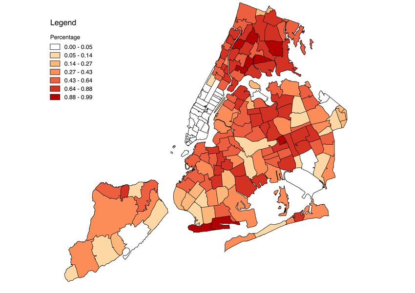
Uber elasticity during the morning rush hour between 6am and 9am in weekday, and 3.9%
during the weekend. In the other boroughs than Manhattan, we estimate 4.6% Uber elasticity
during the morning rush hour, and 9.7% during the weekend. This is an empirical evidence
that Uber turns out to be a substitute for the morning rush hour Yellow cab passenger. We
observe an opposite pattern in the Uber elasticity of Green cab trip demand. In the other
boroughs, the Uber elasticity is about 5.3% during the morning rush hour, and -6.5% during
the weekend. This result can be interpreted as which; for Green cab passengers, Uber is a
complement during the morning rush hour; but it turns out to be a substitute during the
weekend. These Uber elasticity estimates by different hours of day and weekday/weekend
have, however, too big overid test statistics to accept them as supporting evidences.
    The most closely related literature on taxi supply side is Farber (2015) and Brodeur and
Nield (2016). They examine the NYC cabdrivers’ labor supply, one of the famous behavioral
economic subjects established by Camerer et al. (1997), Farber (2008), and Crawford and
Meng (2011). Farber (2015) revisits this issue and show wage elasticity of NYC cabdrivers’
labor supply is positive, which is a neoclassical labor supply model’s prediction. He observes
that; when it rains, number of taxi trips in NYC increases while the total fare income does
not change; and examines the cabdrivers’ heterogenous preference may yield negative wage
elasticity. Brodeur and Nield (2016) examine Uber drivers’ labor supply behavior using a
similar research design to Farber (2015) that Uber rides substantially increases when it rains.
They find that number of daily Uber rides increases in rainy day, and conclude that is an
empirical evidence of which Uber drivers positive respond to demand increase. The validity
of our instrumental variables relies on the positive rain effect on Uber and medallion taxi
rides.
    The other closely related literature on taxi demand side is Cohen et al. (2016) and
Buchholz (2016). Using a large-scale individual Uber trip record data, Cohen et al. (2016)
estimate demand elasticities of Uber and the associated consumer surplus in the four U.S.
cities (New York, Chicago, Los Angeles, and San Francisco). They use Uber’s surge pricing
algorithms to identify price elasticity of Uber at each price point, and obtain a consumer
surplus estimate from the price elasticity estimates. Unlike to Cohen et al. (2016), we focus
on estimating Uber elasticity on medallion taxi demand in this study, instead of estimating
price elasticities of Uber and medallion taxi. Buchholz (2016) demonstrates consumer surplus
of taxi in NYC with respect to search friction and regulated taxi fare. He shows that if search
friction is removed, which is similar to Uber, consumer surplus is doubled by substantially
increasing number of daily trips (matched taxi supply and demand).
    Random utility maximization (RUM) has been a predominant model in travel demand
literature, since the seminal work by Domencich and McFadden (1975), McFadden (1974).

                                              3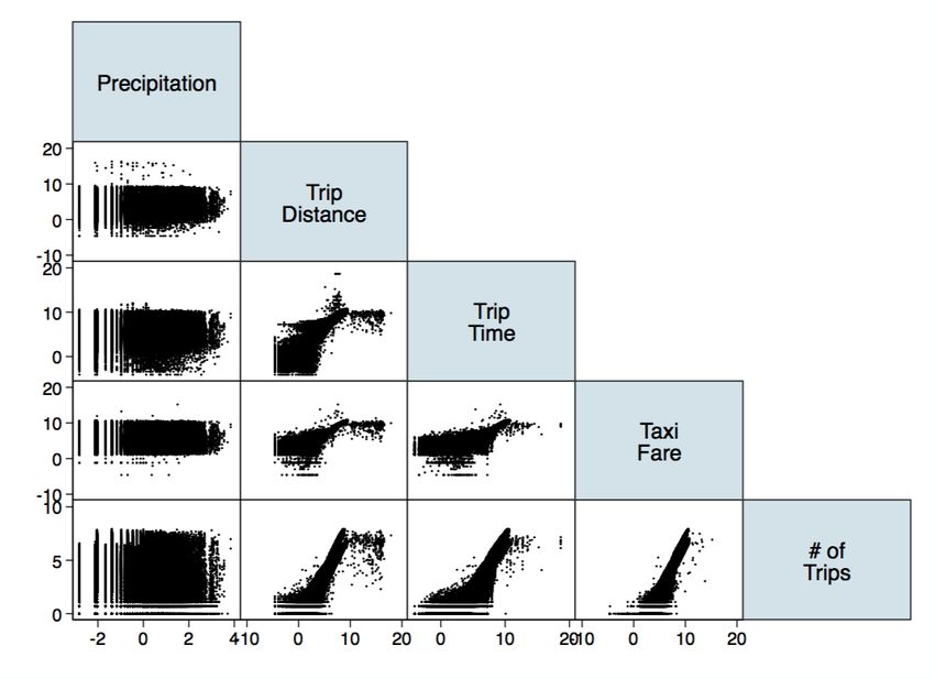
We use an aggregate version of the travel demand model, proposed by Peters et al. (2011).
In this paper, we develop a demand model for trip count with a single trip mode. By using
the count demand model; we can estimate a model for travel demand by taxi as the single
trip mode; and the Uber elasticity of the taxi trip demand. Taxi trip market papers such
as Douglas (1972), De Vany (1975), Beesley and Glaister (1983), Cairns and Liston-Heyes
(1996), Arnott (1996), and Flores-Guri (2003) use the taxi trip demand but different model
specifications. These studies analyze taxi trip market with taxi trip fare as a unit price of
the trip, and discuss whether the regulated fare yield the second best in terms of efficiency
because monopoly pricing would rise due to medallion licensing as an entry control.
    Jackson and Schneider (2011) and Schneider (2010) examine the New York City taxi
drivers’ moral hazard which motivates the drivers to engage in risky driving and criminal
activities. The unit of observation in these studies, however, is the individual driver’s legal
record, not individual taxi trips.

2     The Empirical Framework
The main goal is to estimate the elasticity of NYC medallion cab demand with respect to
Uber. In order to consider spatiotemporal variation, we estimate a panel data model for taxi
trip demand

                             yit = xit β + δ · uit + γi + θt + it ,                        (2.1)

where yit is a number of NYC medallion trips, uit is a number of Uber trips, xit is a vector of
medallion trip attributes, γi and θt are location and time specific effects respectively. The unit
of location for i is NYC zipcode, and hour of day of month of year is for t. The main focus is to
estimate δ by controlling for endogenous Uber demand and medallion taxi trip attributes due
to the cab drivers’ labor supply behavior. Non-uniform, and nonstationary spatiotemporal
variation of the taxi trip demand, in addition, is another factor to be considered in the δ
estimation. By using log of yit and uit , the δ estimate implies the elasticity.

2.1    Data
We use the NYC medallion taxi trip records and the Uber pick-up records from April to
September 2014, and January to June 2015. Both taxi trip records were collected by the
NYC Taxicab & Limosine Commission (TLC), the NYC’s taxi regulatory agency. The NYC
medallion taxi cab consists of official taxicab vehicles (Yellow cab) and street hail livery

                                                  4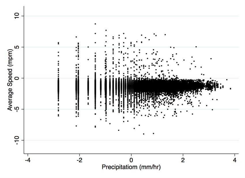
Table 1: Descriptive Statistics

                      #of pick-ups                     Total Fare            Total Trip Distance
             Yellowcab Greencab       Uber      Yellowcab      Greencab     Yellowcab Greencab
  Median      440,246     47,700     40,520     $6,946,085     $703,083     1,378,623     136,663
  Std. dev 53,393.084 14,838.045 29,783.888 $859,212.970 $229,988.996 8,073,866.198 45,088.851
  Max         544,519     81,574    136,193    $10,000,912    $1,569,859    60,720,968    244,962
  Min          0.000      0.000       0.000       $0.000        $0.000        0.000        0.000
  Total Sum 159,481,189 17,166,393 18,804,806 $2,496,244,821 $254,233,258 1,516,589,012 50,496,604
     Note: Std. dev, Max, and Min stand for standard deviation, maximum and minimum value respec-
     tively. Median, Standard deviation, Minimum, and Maximum are daily taxi statistics. Total sum is
     for the entire dataset.

(Green cab). The medallion cabs’ individual trip records are open to the public from the
TLC’s website. The medallion cab trip records have detail information about individual taxi
trip such as pick-up and drop-off date/time, pick-up and drop-off location in GPS coordinates
(latitude and longitude), trip distance, itemized fares, number of passengers and etc. The
Uber trip records, however, are not publicly available from the TLC’s website, so we use the
Uber trip records provided by FiveThirtyEight that have pick-up time and location only.
    Over the sample period, Uber’s market share is around 10% to the NYC taxi trip market.
Descriptive statistics for the daily taxi trip records are reported in Table 1. The median
number of daily pick-ups, at the first row of left panel, are about 5 million for Yellow cab,
six hundred thousand for Green cab, and sixty two hundred thousand. The median total
taxi fare of daily trips, at the first row of the middle panel, are about 82 million dollars for
Yellow cab, and 8 million dollars for Green cab. The median total distance of daily trips,
at the first row of right panel, are about 51 million miles for Yellow cab, 2 million miles for
Green cab. The total number of trips over the sample period, at the fifth row of left panel,
are about 159 million for Yellow cab, 17 million for Green cab, and 19 million for Uber.
    We aggregate individual trip records of Yellow cab, Green cab, and Uber by pick-up
zipcode and hour of day of month of year. By doing so, we can merge them to have matched
records for the three taxi trip services by pick-up zipcode and hour of day of month of
year. 248 unique NYC zipcodes areas are used as a location identifier. We assign zipcode
to the individual trip record according to its pick up geographic coordinates (longitude and
latitude). The zipcode assignment for Uber pick-up is the same for the 2014 records. The
2015 Uber records have “taxi zone identifiers”, instead of the pick-up coordinates. We thus
assign zipcode to the 2015 Uber trip records according to the most overlapped taxi zone.
There are 364 days and 12 months over the sample period. The total number of time points,

                                                  5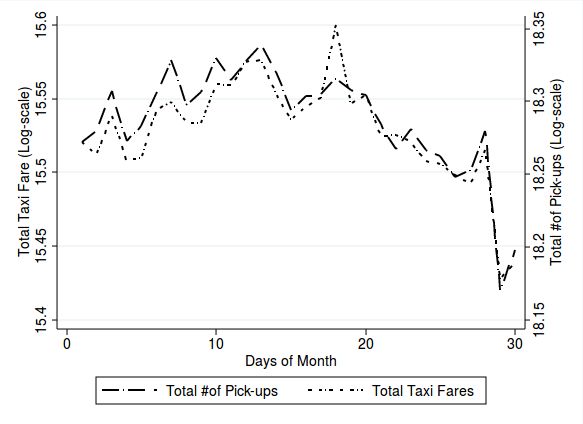
which are hours of days of months of years, is 8,736. The total number of observations is
2,166,528 with which 248 zipcode areas are placed for every time point.
    The rain data that we use for an instrumental variable is hourly precipitation accumu-
lation in millmeter by four square kilometer boundary grid over NYC. This precipitation
data have been produced by the National Centers for Environmental Prediction (NCEP)
stage IV radar. The weather radar measures three meteorological quantities (reflectivity,
radial velocity, and spectrum-width base) per grid. Hourly precipitation accumulation per
grid then is calculated based on the three quantities. The stage IV radar has 1121 × 881
grids covering the entire U.S. territories in North American continent. We identify 189 out
of 1121 × 881 stage IV radar grids covers NYC area, and use the hourly precipitation data
of them for our empirical analysis.3

2.2    Identification
The regression model (2.1) is a demand model, and therefore controlling for endogeneity
due to unobservable supply is crucial to identify the parameters in the model. We use
hourly precipitation in millmeter and dummy variables for pick-up zipcodes as instrumental
variables for number of Uber trips and the endogenous medallion taxi trip attributes such
as trip distance and time, and number of passengers.
    We argue that rain and pick-up location of taxi trips are valid instruments because;
i) taxi trip demand is highly correlated with rain; ii) but the cab drivers’ labor supply is
uncorrelated with rain because of the compliance rule for any passengers’ trip request. Farber
(2015) and Brodeur and Nield (2016) are the first work of examining the rain effect on NYC
taxi cab and Uber drivers’ labor supply respectively. Farber (2015) find that taxi demand
substantially increases when it rains, but drivers’ income does not change. This is due to
decreasing taxi trip supply, according to Farber (2015); because i) traffic congestion gets
worse when it rains; and ii) drivers less prefer to drive under the rain so that they tend to
stop their shift early. Brodeur and Nield (2016) documents an empirical evidence that Uber
drivers positively respond to increasing demand when it rains. And, the magnitude of the
Uber drivers’ response is substantially greater than the NYC medallion cab driver.
    Despite of the consensus on increased taxi trip demand when it rains, the rain effect on
taxi supply still has room to examine. We argue that taxi trip supply is uncorrelated with rain
due to the compliance rule. The TLC mandates drivers to accept any trip requests; unless
the vehicle is occupied and the passengers do not want to pick-up additional passengers; or
  3
    See Hamidi et al. (2017) for more details about the stage IV radar data. Many thanks to Ali Hamidi
and Naresh Devineni at NOAA/Cooperative Remote Sensign Science and Technology Center at the City
College of New York for sharing the Stage IV radar data.

                                                  6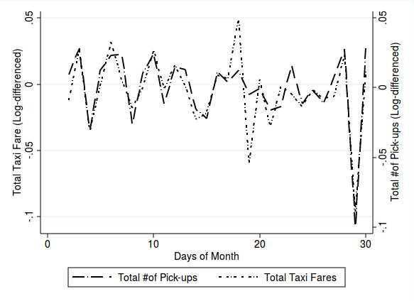
(a) Rain and Taxi Speed                        (b) Rain and Taxi Trip Attributes

                      Figure 1: Scatterplot: Rain and Taxi Trips (Log-scale)

passengers seem to carry harmful objects that would damage the vehicle. According to the
TLC rulebook, “a driver shall not seek to ascertain the destination of a passenger before such
passenger is seated in the taxicab.” 4
    We revisit the rain effect on taxi trip supply and find that precipitation is almost uncor-
related with average speed of taxi trip. As shown in Figure 1(a), the scatterplot of average
taxi trip speed is almost flat on precipitation. We further find that; log of precipitation is
positively correlated with (log of) number of taxi trips (0.0081); and negatively correlated
with trip distance (-0.0018), trip time (-0.0040), and total fare (-0.0013). These correlation
coefficients rather support that taxi trips become more frequent and short when it rains. The
magnitudes of the correlation coefficients are, however, too small to be treated as significant
on, as shown at the first column of the scatterplot matrix in Figure 1(b).

2.3      Spatiotemporal Distribution
To control for nonstationarity issues, we apply the first-differencing transformation by day
of month of year for all variables in (2.1). Number of NYC medallion taxi trips and Uber
trips are nonstationary over time. The time variations of taxi pick-up such as day and night
shifts, and rush hours are quite well known phenomena. The cab drivers’ income targeting,
addressed by a number of behavioral economics papers, effects also on the nonstationary taxi
trip. Farber (2015), in particular, demonstrates the time variation of the NYC medallion
cab. He shows that day shift cab drivers have less flexible begin time, whereas end time is
  4
      See TLC (2010) for more details about rules and regulations for the NYC Yellow cab and Green cab.

                                                    7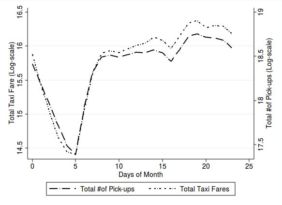
1
    13
    12

                                                                                                              .5
    11

                                                                                                              0
    10

                                                                                                              −.5
    9

   01apr2014                        01jul2014   01oct2014          01jan2015      01apr2015   01jul2015       01apr2014                          01jul2014   01oct2014          01jan2015    01apr2015   01jul2015
                                                            date                                                                                                         date

                                                 Medallion cab                   Uber                                                                         Medallion cab                 Uber

                                   (a) Time Series Plot (Log-scale)                                                                          (b) Time Series Plot (Log-differenced)
                13.5

                                                                                                                             .2
   Number of Medallion Trips

                                                                                                                 Number of Medallion Trips
                       13

                                                                                                                         −.2          0
      12.5

                                                                                                               −.4
                12

                                                                                                                             −.6

                               9                10                          11                   12                                             −.5                         0                              .5
                                                     Number of Uber Trips                                                                                        Number of Uber Trips

                                      (c) Scatterplot (Log-scale)                                                                               (d) Scatterplot (Log-differenced)

                               Figure 2: (Aggregate) Time Variation: Medallion Taxi pick-up and Total Fare

not flexible for night shift drivers.5 Econometric estimation with nonstationary data may
cause either inconsistent target parameter estimation due to serially correlated error term,
or inefficient standard error estimation due to heteroskedasticity.
    In our dataset, daily variation of taxi trip may cause the nonstationarity issue. Figure
2(a) is time series plots for number of NYC medallion cab trips and Uber trips by day. We
can see that Uber trip has steady growth trend while NYC medallion cab is stable. These
different long-run trends may interrupt to estimate the causal relationship between NYC
medallion and Uber trip. The scatterplot of first differenced variables in Figure 2(d) shows
a clear positive linear relationship, which does not appear in Figure 2(c).
    By looking at the spatial distribution of the taxi trip data, we can see that the three
NYC taxis serve for different area. Uber and Green cab pick-up occurred in wider areas than
   5
    Farber (2015) finds that there are two peaks in hourly distribution of shift start time. This is another
evidence that the time variation of NYC taxi trips is nonstationary.

                                                                                                          8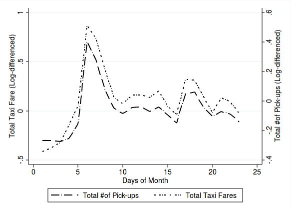
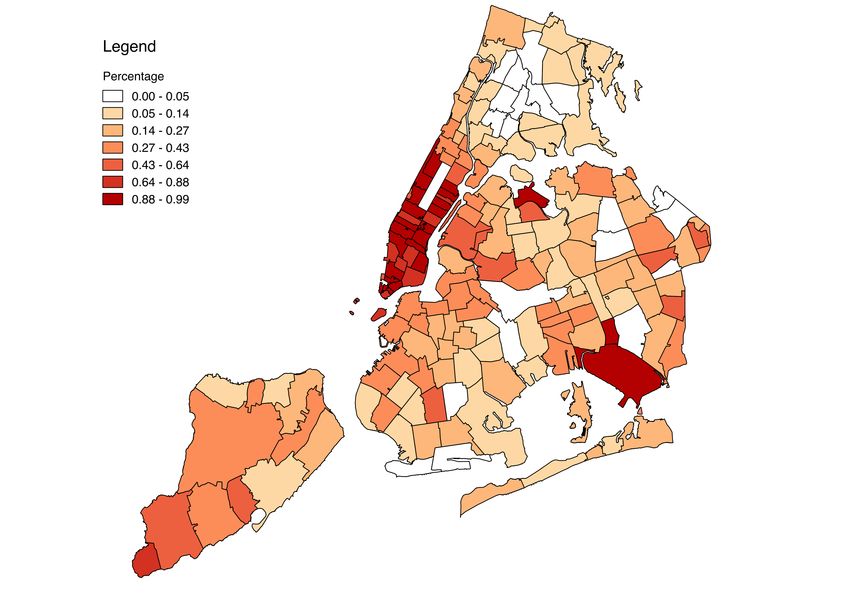
(a) Yellow cab pick-up                      (b) Green cab pick-up

                         (c) Uber pick-up

Figure 3: Spatial Distribution: Proportion of pick-up by Zipcode

                                9
Table 2: Model Estimates with Log-Differenced Variables
# of Taxi Pickups by hour and zipcode
Yellowcab Greencab
OLS TSLS GMM OLS TSLS GMM
Uber 0.0242*** 0.0706*** 0.0466** 0.0154*** 0.1127*** 0.0912***
(Log-differenced) [0.000] (0.017) (0.018) [0.001] (0.027) (0.025)
Trip distance -0.0895*** -0.2494*** -0.2407*** -0.0906*** 0.0543* 0.0212
(Log-differenced) [0.004] (0.053) (0.063) [0.005] (0.029) (0.027)
Trip time 0.1017*** 0.1044** 0.0674** 0.0461*** 0.0209 0.0170***
(Log-differenced) [0.002] (0.047) (0.032) [(0.001] (0.013) (0.004)
Passengers 0.4463*** 0.5316*** 0.6236*** 0.4603*** 0.4810*** 0.4932***
(Log-differenced) [0.002] (0.027) (0.045) [0.002] (0.035) (0.043)
Meter fare 0.4514*** 0.5269*** 0.4800*** 0.4841*** 0.3177*** 0.3513***
(Log-differenced) [0.006] (0.052) (0.096) [0.007] (0.053) (0.063)
Tip -0.0420*** -0.0469*** -0.0388*** -0.0401*** -0.0359*** -0.0363***
(Log-differenced) [0.001] (0.004) (0.007) [0.001] (0.004) (0.005)
Constant -0.0238*** -0.0297*** -0.0177** -0.0243*** 0.0065 0.0010
[0.002] (0.006) (0.008) [0.002] (0.007) (0.007)
# of obs 391,181 391,181 391,181 208,385 208,385 208,385
R2 0.9008 0.8867 0.8787 0.8944 0.8774 0.8837
χ2 Test (df) 375.92(150) 102.70(150) 276.89(126) 74.91(126)
(P-value) (0.0000) (0.9988) (0.0000) (0.9999)
Notes: Standard errors are reported in parentheses. Heteroskedasticity robust standard errors are reported
in square brackets. The symbols, ∗ , ∗∗ , and ∗∗∗ indicate respectively that the estimated coefficient is
statistically significant under 10%, 5%, and 1% significance levels. The TSLS and GMM estimates treat
“# of Uber pickups” , “trip distance”, “trip time”, and “#of passenger”, as endogenous covariates. The
instrumental variables are precipitation and the dummy variables for trip origin ZIP Code . The row for
χ2 Test, 2nd from the bottom, reports the overidentification test statistics with its degrees of freedom
in parentheses. The associated P-values are reported at the bottom in parentheses. Note that all model
estimates contains fixed effect dummy variables for i) months, ii) years, and iii) weekdays.
Yellow cab in NYC. Figure 3 presents the NYC taxi zone maps for the median proportion
of daily pick-ups by zipcode. The Yellow cab pick-up had mostly occurred in Manhattan
below Central park and a few other areas such as airports, whereas Uber and Green cab have
relatively wider pick-up distributions. Note that the Green cabs are restricted to pick-up
passengers up to Central park Manhattan, except special situations, and NYC airports.6
This is the reason that Green cab has almost no daily pick-ups in that area and the airports
as shown in Figure 3(b).
3 Empirical Results
Table 2 reports estimation results of the model (2.1). Three columns on the left panel are the
model estimates for Yellow cab trip, and the three on the right are for Green cab trip. The
Recall that Green cab’s restriction is not to pick-up passengers in Manhattan below west 110th street
6
and east 96th street, the north end of Central Park, and the two NYC airports. See TLC (2013).
10data is a panel data with hours of days of months of year as its time unit. And the spatial
unit is the 5-digit zip code polygon in NYC. Note that all variables, excluding indicators,
are log-differenced from day ago. Since all the variables are in log scale, each coefficients
implies elasticity of each variable.
Overall, we estimate 4.7% Uber elasticity of Yellow cab trip, and 9.1% Uber elasticity
of Green cab trip. These positive and statistically significant coefficients imply that Uber is
a complement for both Yellow cab and Green cab passengers. In particular, one additional
Uber trip causes 4.7% of an additional Yellow cab trip, and 9.1% of an additional Green
cab trip. We choose the GMM estimates and interpret them as our main result. The three
different estimations report different Uber elasticity coefficients for each Yellow cab and
Green cab trip. The sign and statistical significance are, however, not different in all three
estimates.
Our identification strategy aims to control for endogenous cab drivers’ labor supply, and
nonstationary taxi pick-up. The GMM estimates seem to achieve the goal, and provide reli-
able and statistical consistent Uber elasticity estimates. By looking at the overidentification
(overid) test statistics, we can see that the TSLS results strongly reject the null hypothesis
in which the instrumental variables are exogenous, but GMM results do not. These overid
test statistics do not mean that our instrumental variables are invalid. Rather, it means that
heteroskedasticity due to nonstationary data cause rejecting the overidentifying restriction
in TSLS.
The heteroskedasticity seems to come from hourly variation, which is nonstationary, and
the GMM can successfully controls for it. Daily variation of the log-differenced variables that
we use are (relatively) stationary, but their hourly variations do not. Figure 4 show daily
and hourly variations of number of pick-ups and total fare before and after log-differencing.
By looking at panel 4(a) and 4(b), the log-differencing makes daily variation stationary
in which the data series randomly fluctuated around zero. The log-differencing for hourly
variation, however, seems to amplify morning and evening rush hour, which is nonstationary.
By looking at panel 4(c) and 4(d), the log-scale variable series substantially decline in night
time. Their log-differenced series seem to have two peaks, one at morning rush hours between
6am and 9am, and the other at evening rush hours between 5pm and 7pm.
The Uber elasticity of Green cab is twice bigger than that of Yellow cab. This differ-
ence comes from different market share by NYC Borough that Yellow cab and Green cab
differently have. As shown in Table 3, about 91% daily Yellow cab trips and 72% daily
Uber trips occurred in Manhattan below 110th street, whereas only 7% of Green cab trips
occurred in that area. The 4.7% Uber elasticity of Yellow cab trip is therefore mostly made
in Manhattan below 110th street, and 9.1% Uber elasticity of Green cab trip is made mostly
11(a) Day of Month (Log-scale) (b) Day of Month Variation (Log-differenced)
(c) Hour of Day (Log-scale) (d) Hour of Day (Log-differenced)
Figure 4: (Aggregate) Time Variation: Medallion Taxi pick-up and Total Fare
Table 3: Descriptive Statistics: Number of Trips by Borough
Yellow cab Green cab Uber
Median Std.Dev Total Median Std.Dev Total Median Std.Dev Total
th
Below 110 st 386,145 44,875 139,228,280 3,578 1,025 1,237,478 28,928 18,213 12,489,445
Above 110th st 5,234 1,279 1,987,334 10,135 2,710 3,609,152 891 1,132 515,003
Brooklyn 8,356 3,810 3,513,685 16,440 6,567 6,074,914 6,544 5,327 2,811,660
Queens 15,320 2,148 5,563,737 13,023 4,021 4,703,185 2,408 2,858 1,399,821
Bronx 297 117 121,565 3,601 1,144 1,308,222 369 637 254,801
Staten Island 5 4.62 2,064 7 4.94 2,616 15 20 7,992
Airports 8,439 1,169 3,093,857 161 52.1 58,952 828 626 378,678
12Table 4: GMM Estimates of Yellow Cab Demand (# of pick-ups)
Entire sample Manhattan Brooklyn Queens Bronx
All Below 110th Above 110th
Uber 0.0466** 0.0330 0.0407** 0.2278 0.1082 0.1236 0.0344
(Log-differenced) (0.018) (0.022) (0.021) (0.271) (0.097) (0.096) (0.077)
# of obs 391,181 259,791 228,679 31,112 75,543 46,014 1,785
2
R 0.8787 0.8889 0.9208 0.6974 0.8758 0.8173 0.7541
χ2 Test (df) 102.70(150) 14.75(63) 9.90(51) 0.81(8) 19.74(32) 21.40(30) 8.49(11)
(P-value) (0.9988) (1.0000) (1.0000) (0.9992) (0.9556) (0.8751) (0.6690)
Notes: Standard errors are reported in parentheses. Heteroskedasticity robust standard errors are reported in
square brackets. The symbols, ∗ , ∗∗ , and ∗∗∗ indicate respectively that the estimated coefficient is statistically
significant under 10%, 5%, and 1% significance levels.
in Brooklyn and Queens, where 63% Green cab trips occurred.
3.1 Uber Effect on NYC Yellow Cab
Table 4 reports the GMM estimates of the Uber elasticity of Yellow cab trip by borough. We
use the same model specification as Table 2. The estimation results in Table 4 are thus an
extension of the third column in Table 2, the GMM estimate for Yellow cab trip demand. We
perform the GMM estimation by NYC borough, and Manhattan below/above 110th street,
the north end of Central park. The overid test statistics at all seven columns do not reject
the overidentifying restriction, and therefore our instrumental variables are valid one for all
model estimates in Table 4.
The 4.7% Uber elasticity for all NYC Yellowcab trip demand comes mostly from Man-
hattan below 110th street. The Uber elasticity estimate in that area is about 4.1%, reported
at the third column of Table 4. The Uber elasticity estimate in the entire Manhattan is
about 3.3%, and 23% in Manhattan above 110th street. But, neither of both estimates are
statistically significant under 10% significance level. This is an empirical evidence that Uber
is a complement for Yellow cab passengers particularly in Manhattan below 110th street.
The Uber elasticity estimates in the other NYC boroughs than Manhattan are all positive
but statistically insignificant under 10% significance level. The elasticity estimates in Brook-
lyn and Queens have, however, Z-statistics that exceed one. It is thus too early to conclude
Uber has no impact on Yellow cab demand in the other boroughs but Manhattan below 110th
street. We are unable to estimate the elasticity in Staten Island due to insufficient number
of observations.
We estimate the Uber elasticity during rush hours in weekday and weekend, in Manhattan
13Table 5: GMM Estimates for Yellow Cab By Rush Hour and Weekend
Manhattan Below 110th st Manhattan Above 110th st Other Boroughs
Morning Evening Weekend Morning Evening Weekend Morning Evening Weekend
Uber -0.0207** 0.0041 0.0389*** 0.0254 0.1278 -0.0488 0.0458* 0.0443 0.0969***
(0.010) (0.009) (0.008) (0.141) (0.118) (0.086) (0.024) (0.028) (0.028)
# of obs 26,714 24,604 63,605 4,070 3,112 10,115 18,352 11,750 43,390
R2 0.9309 0.8540 0.9139 0.7698 0.8252 0.7647 0.7194 0.8386 0.7587
2
χ Test (df) 79.73(49) 41.67(51) 233.41(51) 1.81(8) 3.00(8) 8.79(8) 88.55(70) 74.09(60) 128.71(78)
(P-value) (0.0036) (0.8213) (0.0000) (0.9863) (0.9346) (0.3607) (0.0665) (0.1043) (0.0003)
Notes: Standard errors are reported in parentheses. Heteroskedasticity robust standard errors are reported in square
brackets. The symbols, ∗ , ∗∗ , and ∗∗∗ indicate respectively that the estimated coefficient is statistically significant under
10%, 5%, and 1% significance levels. Morning rush hour is between 6am and 9am in weekday. Evening rush hour is
between 5pm and 7pm.
below/above 110th street and the other NYC boroughs than Manhattan, reported in Table 5.
Interestingly, we have a negative Uber elasticity estimate in Manhattan during the moring
rush hour between 6am and 9am. The GMM estimate is about -2.1% and it is statistically
significant under 5% significance level. The elasticity estimate for the weekend is about 4%,
which is close to the overall Uber elasticity of Yellow cab trip. The elasticity estimate for the
evening rush hour between 5pm and 7pm is less than 1% but it is not statistically significant
under 10% significance level.
In summary, the Uber elasticity is significant during the moring rush hour and weekend.
And, the morning rush hour elasticity is negative that means Uber is a substitute for the
morning rush hour Yellow cab passengers. However, the overid test statistics for both morn-
ing rush hour and weekend strongly reject the overidentifying restriction. Thus, these two
Yellow cab trip samples need to be re-examined with more observations.
3.2 The Uber effect on NYC Green Cab
Table 6 reports GMM estimates of the Uber elasticity of Green cab during the moring and
evening rush hours in weekday, and during the weekend in Manhattan above 110th street and
the other boroughs than Manhattan. Recall that Green cabs are restricted not to pick-up
passengers in Manhattan below west 110th street and east 96th street. Other regulations
imposed by the TLC are the same for both Yellow cab and Green cab.
In the other boroughs than Manhattan, the Uber elasticity estimate is about 5% during
the moring rush hour, and it is statistically significant under 10% significance level. During
the weekend, however, the elasticity estimate is about -6.5% with statistical significance
under 1% significance level. The weekend elasticity estimate for Green cab has opposite
14Table 6: GMM Estimates By Rush Hour and Weekend
Manhattan Above 110th st Other Boroughs
Morning Evening Weekend Morning Evening Weekend
Uber -0.0080 0.0107 -0.0704 0.0526* -0.0000 -0.0648***
(0.106) (0.086) (0.051) (0.031) (0.018) (0.024)
# of obs 4,346 3,472 10,719 20,802 17,655 52,202
R2 0.8649 0.6257 0.8953 0.8244 0.7760 0.7799
χ2 Test (df) 4.23(8) 0.31(8) 5.65(8) 97.81(75) 91.36(78) 208.95(89)
(P-value) (0.8358) (1.0000) (0.6868) (0.0397) (0.1430) (0.0000)
Notes: Standard errors are reported in parentheses. Heteroskedasticity robust stan-
dard errors are reported in square brackets. The symbols, ∗ , ∗∗ , and ∗∗∗ indicate
respectively that the estimated coefficient is statistically significant under 10%, 5%,
and 1% significance levels. Morning rush hour is between 6am and 9am in weekday.
Evening rush hour is between 5pm and 7pm.
sign with the positive Uber elasticity for Yellow cab. This negative elasticity might be an
empirical evidence that; for Green cab passengers, Uber is a substitute in the other boroughs
than Manhattan during the weekend. But, the Green cab’s negative Uber elasticity estimate
needs to be re-examined with more observations because its overid test statistics show that
strongly reject the overidentifying restriction. There are no statistically significant Uber
elasticity estimates in any time in Manhattan above 110th street.
References
Arnott, R. (1996). Taxi travel should be subsidized. Journal of Urban Economics, 40(3):316–
333.
Beesley, M. E. and Glaister, S. (1983). Information for regulating: the case of taxis. The
economic journal, 93(371):594–615.
Brodeur, A. and Nield, K. (2016). Has uber made it easier to get a ride in the rain? IZA
Discussion Paper No. 9986.
Buchholz, N. (2016). Spatial equilibrium, search frictions and efficient regulation in the taxi
industry.
Cairns, R. D. and Liston-Heyes, C. (1996). Competition and regulation in the taxi industry.
Journal of Public Economics, 59(1):1–15.
Camerer, C., Babcock, L., Loewenstein, G., and Thaler, R. (1997). Labor supply of new york
city cabdrivers: One day at a time. The Quarterly Journal of Economics, 112(2):407–441.
15Chen, M. K., Chevalier, J. A., Rossi, P. E., and Oehlsen, E. (2017). The value of flexible
work: Evidence from uber drivers. Technical report, NBER Working Paper No. 23296.
Cohen, P., Hahn, R., Hall, J., Levitt, S., and Metcalfe, R. (2016). Using big data to estimate
consumer surplus: The case of uber. Technical report. NBER Working Paper No. 22627.
Cramer, J. and Krueger, A. B. (2016). Disruptive change in the taxi business: The case of
uber. The American Economic Review, 106(5):177–182.
Crawford, V. P. and Meng, J. (2011). New york city cab drivers’ labor supply revisited:
Reference-dependent preferences with rationalexpectations targets for hours and income.
The American Economic Review, 101(5):1912–1932.
De Vany, A. S. (1975). Capacity utilization under alternative regulatory restraints: an
analysis of taxi markets. Journal of Political Economy, 83(1):83–94.
Domencich, T. A. and McFadden, D. (1975). Urban travel demand-a behavioral analysis.
Technical report.
Douglas, G. W. (1972). Price regulation and optimal service standards: The taxicab industry.
Journal of Transport Economics and Policy, pages 116–127.
Farber, H. S. (2008). Reference-dependent preferences and labor supply: The case of new
york city taxi drivers. American Economic Review, 98(3):1069–82.
Farber, H. S. (2015). Why you can‘t find a taxi in the rain and other labor supply lessons
from cab drivers. The Quarterly Journal of Economics, 130(4):1975–2026.
Flores-Guri, D. (2003). An economic analysis of regulated taxicab markets. Review of
Industrial Organization, 23(3):255–266.
Hall, J. V. and Krueger, A. B. (2016). An analysis of the labor market for uberâĂŹs driver-
partners in the united states. Technical report, NBER Working Paper No. 22843.
Hamidi, A., Devineni, N., Booth, J. F., Hosten, A., Ferraro, R. R., and Khanbilvardi, R.
(2017). Classifying urban rainfall extremes using weather radar data: An application to
the greater new york area. Journal of Hydrometeorology, 18(3):611–623.
Jackson, C. K. and Schneider, H. S. (2011). Do social connections reduce moral hazard?
evidence from the new york city taxi industry. American Economic Journal: Applied
Economics, 3(3):244–267.
16McFadden, D. (1974). The measurement of urban travel demand. Journal of public eco-
nomics, 3(4):303–328.
Peters, J., Shim, H., and Kress, M. (2011). Disaggregate multimodal travel demand modeling
based on road pricing and access to transit. Transportation Research Record: Journal of
the Transportation Research Board, (2263):57–65.
Schneider, H. (2010). Moral hazard in leasing contracts: Evidence from the new york city
taxi industry. The Journal of Law and Economics, 53(4):783–805.
TLC (2010). Old Rule Book. The New York City Taxi & Limousine Commission.
TLC (2013). Background on the Boro Taxi program. The New York City Taxi & Limou-
sine Commission. http://www.nyc.gov/html/tlc/html/passenger/shl_passenger_
background.shtml.
TLC (2016). 2016 TLC Factbook. The New York City Taxi & Limousine Commission.
http://www.nyc.gov/html/tlc/html/about/factbook.shtml.
17You can also read