ON THE NATURE OF EARTH-MARS PORKCHOP PLOTS
←
→
Page content transcription
If your browser does not render page correctly, please read the page content below
(Preprint) AAS 13-226

        ON THE NATURE OF EARTH-MARS PORKCHOP PLOTS

                            Ryan C. Woolley* and Charles W. Whetsel †

              Porkchop plots are a quick and convenient tool to help mission designers plan
              ballistic trajectories between two bodies. Parameter contours give rise to the
              familiar “porkchop” shape. Each synodic period the pattern repeats, but not ex-
              actly, primarily due to differences in inclination and non-zero eccentricity. In
              this paper we examine the morphological features of Earth-to-Mars porkchop
              plots and the orbital characteristics that create them. These results are compared
              to idealistic and optimized transfers. Conclusions are drawn about “good” op-
              portunities versus “bad” opportunities for different mission applications.

INTRODUCTION
    Plotting interplanetary trajectory parameters such as C 3 and V ∞ in launch-date/arrival-date
space and tracing isometric lines are a valuable mission design tool that are used in optimizing the
trajectories for most interplanetary missions. The most important energy parameters (C 3 and V ∞ )
typically create bi-lobed characteristic shapes which have earned these plots the colloquial nick-
name of “porkchop” plots. Porkchop plots aide early mission designers in selecting launch dates,
in calculating launch energies and ΔV budgets, and visually optimizing trajectories. Launch peri-
ods are designed by applying constraints on some parameters (e.g. launch declination, arrival
dates, launch period duration, entry speed, sun angles) while simultaneously minimizing others
(e.g. launch energy, Mars orbit insertion (MOI) ΔV). 1,2,3
   Each opportunity (~26 months for Earth to Mars) a new porkchop plot is created with similar
characteristics, but with different minima (on either side of the central ridge), minima locations,
ridge width, and lobe shapes. In this paper we investigate how the orbital characteristics of Earth
and Mars affect the nature of the porkchop plots and how they compare to ideal (circular, co-
planar) and optimized (allowing launch, arrival, and transfer time to be free parameters) porkchop
plots. We also explore what defines a “good” opportunity for Mars missions and to what extent
certain characteristics repeat with Mars cycles (approximately 15 years or 7 opportunities) and
super-cycles.

PORKCHOP PLOTS
   Lambert’s Theorem can be used to calculate the orbital parameters of the trajectory between
any two points for a given time of flight (TOF). 4 This means that for any launch date at Earth

*
  Systems Engineer, Pre-Projects Systems Engineering Group, Jet Propulsion Laboratory, California Institute of Tech-
nology, 4800 Oak Grove Drive, Pasadena, CA 91109.
†
  Manager, Mars Advanced Studies and Program Architecture Office, Jet Propulsion Laboratory.
2013 California Institute of Technology. Government sponsorship acknowledged.

                                                           1
(which specifies location 1) and arrival date at Mars (which specifies location 2 and TOF), there
exists a conic trajectory connecting the two. Plotting contours of the relevant parameters of the
connecting trajectories against combinations of launch date and arrival date create a two-lobed
chart known as a porkchop plot. While traditional porkchop plots often portray the specific depar-
ture energy and hyperbolic excess arrival energy individually (C 3 and V ∞ respectively), for the
purposes of this investigation, the authors chose to focus on a combination of these parameters,
termed the “total transfer ΔV”. Figure 1 shows total transfer ΔV (defined in Equation 1, below)
for the 2018 Earth-to-Mars opportunity.

                                    Total ∆ V                                                               15
                   01/10/20
                                                                                                            14

                   10/02/19                                                                                 13

                                                                                                            12

                                                                                                                 Total ∆ V (km/s)
                   06/24/19
    Arrival Date

                                                                                                            11

                   03/16/19                                                                                 10

                                                                                                            9
                   12/06/18
                                                                                                            8

                   08/28/18                                                                                 7

                                                                                                            6
                         09/12/17 11/01/17 12/21/17 02/09/18 03/31/18 05/20/18 07/09/18 08/28/18 10/17/18
                                                           Launch Date

                              Figure 1. 2018 Earth-to-Mars Porkchop Plot with total ΔV contours.

    Trajectories below the central ridge are referred to as Type I trajectories (< 180°), and trajecto-
ries above are Type II’s (>180°). The ridge itself is due to the fact that Earth and Mars do not lie
in the same plane. Hohmann-like transfers, therefore, generally necessitate a large out-of-plane
component which in turn requires a large amount of energy, creating the ridge. When Earth and
Mars are phased properly the trajectory remains in-plane and a “bridge” is formed across that
central ridge.
    Over a larger range of departure and arrival dates we can see that the minima are repeated
each synodic period, as shown in Figure 2. A closer examination of each opportunity reveals that
the lobed structure varies in size and shape, as do the central ridge width and locations (Type I vs.
II) and values of the minimum ΔV trajectory. Since the Earth goes around the sun 2.14 times
each synodic period, the relative geometry of Earth and Mars shifts by 48.7 degrees. 5

                                                                  2
Figure 2. Multiple porkchop plots from 2011-2028 showing changing shape and structure.
Each date on the x and y axes corresponds to perihelion for Earth and Mars, respectively.
Note the location of the minimum ΔV for each opportunity with respect to the squares on
the grid. Every 7 opportunities the minima are in a similar location resulting in a near-
repeat.
OPTIMIZED PORKCHOP PLOTS AND TRANSFERS
In order to compare the quality of trajectories from one opportunity to the next, it is necessary
to choose a figure-of-merit (FOM). This simplifies matters by allowing us to plot one set of con-
tours and to define optimal trajectories. The choice of a FOM is subjective and can be defined by
mission objectives. For our purposes we chose to use the total transfer ΔV as defined by
∆V = VEarth (t1 ) − VT (t1 ) + VMars (t 2 ) − VT (t 2 ) (1)
where t 1 is the time at launch, t 2 is the time at arrival, and V T is the velocity of the transfer trajec-
tory. This is the orbital transfer equation (neglecting gravity at Earth and Mars) and was chosen
because it balances the contributions of C 3 and V ∞.
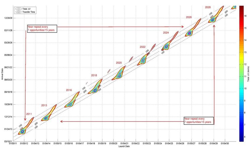
Since Mars is inclined 1.85° to the ecliptic and both Earth and Mars have non-zero eccentri-
cities, true Hohmann transfers are not possible. The actual ephemerides of the planets constrain
the transfer angles and times when other parameters are chosen. If we let launch location (true
anomaly of Earth, ν Earth ), arrival location (true anomaly of Mars, ν Mars ), and transfer time (Δt) be
free variables it is possible to find the ΔV optimized trajectory for each ν Earth -ν Mars pair. Plotting
the contours of minimized ΔV vs. ν Earth and ν Mars (as opposed to launch date/arrival date) creates
an “optimized porkchop plot” that is that is strictly a function of departure and arrival geometry
for Earth and Mars, and is decoupled from time (i.e. makes no assumption about in which real
years or which real launch/arrival opportunities these specific geometric conditions exist).
3Table 1. ΔV Optimized Earth-Mars Transfers
Case 1 Case 2 Case 3 Case 4 Case 5 Actuals (2011-2043)
Parameter Circular Eccentric Rotated Circular Full Best Worst
Co-planar Co-planar Apsides Inclined Model (2026) (2016)
Total ΔV (km/s) 5.59 5.49 5.51 5.66 5.60 5.61 7.12
ΔV 1 (km/s) 2.94 3.40 3.57 2.98 3.06 3.04 3.36
ΔV 2 (km/s) 2.65 2.09 1.94 2.68 2.54 2.57 3.76
Transfer Angle 180° 180° 187° 180° 205.3° 205.7° 214.1°
Transfer Time 259 days 278 days 293 days 259 days 313 days 311 days 277 days
Launch (ν Earth ) n/a 0° 236.4° 306.7° 290.2° 294.2° 13.1°
Arrival (ν Mars ) n/a 180° 190° 253.5° 262.3° 266.8° 354.6°
Eccentricity 0.208 0.258 0.245 0.208 0.221 0.218 0.176
ANALYSIS
This research was carried out using Earth and Mars true anomaly as a coordinate frame for
departures and arrival so that it would be readily apparent how close transfers occur to the apsi-
des. Earth true anomaly can also be used as a surrogate for day of the year since Earth perihelion
typically occurs around January 4 and 365 days is close to 360°. Mars true anomaly is not as en-
lightening, other than to indicate where Mars is with respect to its apsides. Once we note that
Mars line of nodes occurs at ν Mars = 74° and 254° it is easier to see why the most fuel-efficient
trajectories cluster there. Also of interest to mission designers is the Mars season at arrival,
measured by the solar longitude, or L s . Mars L s starts at 0° at its vernal equinox in the same way
that Earth’s vernal equinox starts at the 1st point of Aries – both being related to axial tilt orienta-
tion. The 1st point of Ares is the point of reference for most heliocentric reference frames. It may
be useful to convert the locations presented in this paper into one of these alternate frames of ref-
erence. For this purpose Table 2 is included with the appropriate conversion factors.
Table 2 - Heliocentric Longitudinal Reference Frames and Conversions
Convert From:
Measurement Frame Reference Point
Heliocentric Earth ν Mars ν Mars L s
Heliocentric (Earth L s ) 1st Point of Aries --- +102.9° -23.9° +95.1°
Earth True Anomaly (ν) Earth Perihelion -102.9° --- -126.8° +7.8°
Mars True Anomaly (ν)* Mars Perihelion +23.9° +126.8° --- -119°
Mars Solar Longitude (L s )* Mars Vernal Equinox -95.1° -7.8° +119° ---
*Mars is inclined 1.85° to the ecliptic, rendering these conversions approximate and quasi-linear
The bottoms of the contour troughs on either side of the 180° ridge in the optimized porkchop
plot is are not flat. They are lowest near the bridges and rise to a saddle on either side of the ridge
somewhere in between the two bridges. Since most real transfers are not able to take place at the
global optimum, it is useful to know when Type I is better than Type II, and vice versa. For Case
4, where the orbits are inclined but circular, the troughs are symmetrical about the ridge when
sampled perpendicularly (see Figure 9a). However, when sampled on either side along the same
Earth true anomaly they are not symmetric. Figure 9c shows the minimum ΔV’s vs. Earth true
anomaly for both Type I and Type II trajectories. The asymmetry along the true anomaly lines
9The minimum ΔV transfer in each case are within 30 m/s of each other, but since Mars’ periheli-
on is 74° from the ascending node and 116° from the descending node they are not symmetric and
Type II is slightly more favored. *
The eccentricity of the orbits causes the local minimum near the bridges to move away from
the line of nodes. This causes the bridges to no longer be switching points between trajectory
type regions – reducing their number from four to two. As can be seen in Figure 9d, Type I tra-
jectories are favored earlier in the year with Type II being favored later. The peaks at the switch-
ing points are also asymmetrical with the one at ν Earth = 50° reaching 7.4 km/s and the one at ν Earth
= 230° reaching 6.7 km/s. Actual trajectory optima for the years 2011-2180 are plotted as data
points. Note the absence of trajectories around the first switching point peak.
Comparison to Actual Data
It is possible to plot the actual ephemerides of Mars onto the optimized porkchop plot in terms
of where Mars is with respect to Earth. Since the ratio of one Earth period to one Mars period is
365 days vs. 687 days, the slope on the n-n plot would be 365/687 = 0.53, or about ½, with some
variation due to eccentricity. It would be more instructive to plot the location of Mars around
200-300 days in the future – roughly the length of optimal transfers. These isochrones would be
parallel and cross the region of optimal transfer angles (the troughs on either side of the 180°
transfer ridge, which has a slope of 1 on this plot) once every synodic period (~26 months).
When the isochrones of the true ephemeris are equal to the optimal transfer times (of Figure 8b)
for a given ν Earth -ν Mars pair, the transfer ΔV is equal to the optimal ΔV at that point.
Of course, the majority of the time the optimal transfer locations and transfer times will not
exactly coincide. The regions where the actual transfer times and transfer locations approach
those of the optimal porkchop plot then create the bi-lobed structure of the opportunity-specific
porkchop plot. Actual porkchop plots for the Earth-Mars opportunities between 2011 and 2180
were created and the locations for optimized transfer ΔV were found. The data points are plotted
on Figure 9b and Figure 9d, and the parameters up through 2073 are listed in Table 3. Note that
they come quite close to the true minima, but not quite. It is also notable that the trajectories
“avoid” the peak around ν Earth = 20-70° and tend to be more dense around the global minimum
Type II trajectory.
*
The location of Earth perihelion also plays a role.
11Table 3 - Optimal ∆V Transfers for 2011-2073
Year ∆V Tot ΔV 1 ΔV 2 ν Earth ν Mars Transfer T angle Type e LD AD
km/s km/s km/s deg. deg. days deg.
2011 5.70 2.99 2.70 303.1 278.5 307 208.6 2 0.210 11/9/2011 9/11/2012
2013 6.24 3.07 3.17 330.8 312.4 295 214.7 2 0.190 12/6/2013 9/27/2014
2016 7.12 3.36 3.76 13.1 354.0 277 214.1 2 0.176 1/17/2016 10/20/2016
2018 5.76 2.80 2.96 128.0 47.6 204 152.8 1 0.175 5/12/2018 12/2/2018
2020 6.32 3.71 2.61 199.2 112.6 205 146.5 1 0.231 7/25/2020 2/15/2021
2022 6.49 3.84 2.65 236.2 215.4 351 212.3 2 0.251 9/2/2022 8/19/2023
2024 5.82 3.36 2.45 265.9 242.0 334 209.3 2 0.237 10/2/2024 9/1/2025
2026 5.61 3.04 2.57 294.2 266.8 311 205.7 2 0.218 10/31/2026 9/7/2027
2028 5.99 3.02 2.97 318.8 298.8 301 213.2 2 0.198 11/24/2028 9/21/2029
2030 6.75 3.22 3.53 353.8 336.3 285 215.7 2 0.180 12/29/2030 10/10/2031
2033 6.33 3.00 3.33 102.8 17.4 198 147.8 1 0.167 4/16/2033 10/31/2033
2035 5.85 3.21 2.64 170.7 86.4 201 148.8 1 0.208 6/26/2035 1/13/2036
2037 6.85 4.03 2.82 223.8 203.3 354 212.7 2 0.254 8/20/2037 8/9/2038
2039 6.03 3.54 2.49 254.3 232.0 342 210.9 2 0.243 9/21/2039 8/28/2040
2041 5.62 3.13 2.48 283.3 256.5 319 206.3 2 0.226 10/20/2041 9/4/2042
2043 5.79 3.00 2.79 308.8 285.7 305 210.1 2 0.206 11/15/2043 9/15/2044
2045 6.41 3.11 3.30 338.7 320.9 292 215.4 2 0.186 12/14/2045 10/2/2046
2048 6.95 3.26 3.69 76.3 350.2 199 147.1 1 0.171 3/20/2048 10/5/2048
2050 5.63 2.83 2.80 141.2 62.4 206 154.4 1 0.185 5/26/2050 12/18/2050
2052 6.59 3.98 2.61 213.3 126.6 210 146.5 1 0.241 8/9/2052 3/7/2053
2054 6.31 3.73 2.58 242.7 221.3 348 211.9 2 0.248 9/9/2054 8/23/2055
2056 5.72 3.27 2.45 272.5 247.0 328 207.6 2 0.233 10/9/2056 9/2/2057
2058 5.65 3.01 2.64 298.9 272.6 308 207.0 2 0.214 11/5/2058 9/9/2059
2060 6.13 3.04 3.08 325.6 306.5 298 214.1 2 0.194 12/1/2060 9/25/2061
2063 6.95 3.29 3.66 3.7 345.8 281 215.4 2 0.178 1/8/2063 10/16/2063
2065 5.98 2.86 3.12 117.1 34.3 201 150.4 1 0.169 5/1/2065 11/18/2065
2067 6.10 3.49 2.61 187.6 101.1 202 146.7 1 0.222 7/14/2067 2/1/2068
2069 6.64 3.91 2.72 231.2 210.5 353 212.5 2 0.252 8/28/2069 8/16/2070
2071 5.90 3.44 2.46 260.8 237.3 337 209.7 2 0.239 9/28/2071 8/30/2072
2073 5.60 3.08 2.52 290.0 261.6 313 204.8 2 0.222 10/27/2073 9/5/2074
CONCLUSIONS AND FUTURE RESEARCH
The nature of Earth-Mars porkchop plot morphology and how it varies from opportunity to
opportunity was investigated by the authors. Total transfer ΔV was used as a surrogate FOM that
is used to optimize trajectories and to compare to actuals. The “best” trajectory of each oppor-
tunity varies from near-optimal up to 30% worse for the total ΔV FOM. The actual impact of
these variances on interplanetary mission design is often a strong function of the mission objec-
tives and propulsion technology. Orbiters utilizing chemical propulsion are most sensitive to the
required ΔV both leaving Mars and upon arrival, although aeroassist techniques (aerobraking,
12aerocapture) minimize the penalties associated with higher arrival velocities. Direct entry landed
missions are typically much less sensitive to arrival velocity as long as constraints such as the
maximum allowable heating rate and total heat load to their entry aeroshells can be maintained
within the arrival conditions. Alternate FOMs should be investigated to determine the optimality
of trajectories for different mission applications which may take into account things such as trans-
fer time, launch declination, arrival date, entry speed, etc.
Earth-Mars geometry roughly repeats every 15 years, or 7 opportunities. However, the subtle
differences in true anomalies amplify the effects of inclination, eccentricity, and transfer time, so
as to make repeatability of most specific trajectory parameters crude at best and non-existent at
worst, although “representative regions” of the porkchop plot coordinate space repeat from op-
portunity to opportunity. Applying constraints to these parameters to meet mission requirements
further exacerbates the challenges of finding “exact repeats.”
This type of comparative analysis across multiple launch opportunity has greatest utility dur-
ing the earliest phases of planning for a mission or series of missions when programmatic uncer-
tainties preclude detailed planning for a specific opportunity. Better understanding of the varia-
bility from opportunity to opportunity allows mission and system architects to better scope by
how much the key mission-driven parameters of the system may vary depending on the selected
opportunity, or, if programmatic robustness or flexibility to design a system capable of launching
in more than one candidate launch opportunity is mandated, this type of analysis could prove in-
valuable.
Another pathway for future investigation is the opposite of mission specific applications of
this research. Rather, it would be to further generalize the analyses presented in this paper to
transfers between any two orbits. This would shed further light on the effects of orbital parame-
ters on optimal transfers and the morphology of FOM contours. The key parameters of optimal
transfers (ΔV 1 , ΔV 2 , locations, etc.) are derivable from e 1 , e 2 , Δi, and Γ. Much exists in the lit-
erature on numerical methods for trajectory optimization. However, it would be instructive to
formalize analytically, visually, and algebraically the relationships between orbital parameters
and optimal transfers.
ACKNOWLEDGMENTS
This research was carried out at the Jet Propulsion Laboratory, California Institute of Tech-
nology, under a contract with the National Aeronautics and Space Administration. Government
sponsorship acknowledged.
REFERENCES
1
A.B. Sergeyevsky, G.C. Snyder, and R.A. Cunniff, “Interplanetary Mission Design Handbook. Volume I, Part 2:
Earth to Mars Ballistic Mission Opportunities, 1990-2005”, JPL Publication 82-43, September 15, 1983.
2
S. Matousek and A.B. Sergeyevsky, “To Mars and Back: 2002-2020. Ballistic Trajectory Data for the Mission Archi-
tect”, AIAA 98-4396, AIAA/AAS Astrodynamics Specialist Conference, Boston, MA, August 10-12, 1998.
3
L.E. George and L.D. Kos, “Interplanetary Mission Design Handbook: Earth-to-Mars Mission Opportunities and
Mars-to-Earth Return Opportunities 2009-2024”, NASA/TM-1998-208533, 1998.
4
D.A. Vallado, Fundamentals of Astrodynamics and Applications, Space Technology Library, Microcosm Press, El
Segundo, California, 2001.
5
C.F. Capen, “A Guide to Observing Mars”, Strolling Astron., Vol. 30, Nos. 9 - 10, p. 186 – 190, 1984.
136
C.H. Won, "Fuel- or Time-Optimal Transfers Between Coplanar, Coaxial Ellipses Using Lambert's Theorem", Jour-
nal of Guidance, Control, and Dynamics, Vol. 22, No. 4, pp. 536-542, 1999.
14You can also read