Optical solitons via the collective variable method for the classical and perturbed Chen-Lee-Liu equations - De Gruyter
←
→
Page content transcription
If your browser does not render page correctly, please read the page content below
Open Physics 2021; 19: 559–567
Research Article
Reyouf Alrashed, Aisha Abdu Alshaery*, and Sadah Alkhateeb
Optical solitons via the collective variable
method for the classical and perturbed
Chen–Lee–Liu equations
https://doi.org/10.1515/phys-2021-0065 munication and optical fibers. In addition, solitary wave
received July 03, 2021; accepted August 13, 2021 solutions or solitons are important structures of evolution
Abstract: In this article, the collective variable method to equations with fascinating characteristics that occur in
study two types of the Chen–Lee–Liu (CLL) equations, is various forms and have great uses. One of the renowned
employed. The CLL equation, which is also the second equations in this category is the Chen–Lee–Liu (CLL)
member of the derivative nonlinear Schrödinger equa- equation [8] which emerged in 1979. CLL equation which
tions, is known to have vast applications in optical is also the second member of the derivative nonlinear
fibers, in particular. More specifically, a consideration Schrödinger equations is known to have many applica-
to the classical Chen–Lee–Liu (CCLL) and the perturbed tions in optical fibers and in the sub-picosecond soliton
Chen–Lee–Liu (PCLL) equations, is made. Certain gra- propagation, in particular. Due to its interesting applica-
phical illustrations of the simulated numerical results tions, CLL model has over the years undergone various
that depict the pulse interactions in terms of the soliton extensions, modifications, and perturbations in relation
parameters are provided. Also, the influential parameters to different situations and applications [9–14]. Besides,
in each model that characterize the evolution of pulse optical soliton perturbation is one of the most energetic
propagation in the media, are identified. areas of study in the areas of telecommunication technology
and physics [15–22]. Furthermore, there exist various com-
Keywords: CLL equations, perturbation term, collective putational, semi-analytical, and analytical techniques to
variables method, solitons treat different forms of nonlinear Schrödinger equations
including the computational Adomian’s method [23–25],
tanh function expansion method [26,27], certain integra-
tion schemes [28], Kudryashov method [29], rational (G/G)-
1 Introduction expansion method [30], trial equation approach [31],
sine-Gordon equation approach [32], and many more
Nonlinear Schrödinger equations are complex-valued time- [33,34] to mention a few.
evolving equations that are known to have a variety of Furthermore, a method of interest in this article is the
applications in nonlinear sciences including biological collective variable method [35–43]. In the given refer-
models, optics, fluid dynamics, plasma physics, among ences, different researchers have over a time employed
other fields [1–7]. Hyperbolic function solutions of these the collective variable method to examine various evolu-
equations or rather solitary wave solutions which are also tion and Schrödinger equations. This method is relatively
referred to as solitons are found to play a vital role in a new technique that splits the complex-valued wave
many pulse propagation processes in modern telecom- function into two components and thereafter introduces
new variables to characterize the dynamics of soliton
propagation. Additionally, the method which was first
introduced by Boesch et al. [44] is a mixture of an analy-
tical process with a computational technique or semi-ana-
* Corresponding author: Aisha Abdu Alshaery, Department of lytical process to analyze the model under consideration.
Mathematics, Faculty of Science, University of Jeddah, Jeddah,
Above and beyond, the method gives the dynamics of each
P.O. Box 80327, Saudi Arabia, e-mail: aaal-shaery@uj.edu.sa
Reyouf Alrashed, Sadah Alkhateeb: Department of Mathematics,
of the pulse parameter by utilizing the Gaussian ansatz to
Faculty of Science, University of Jeddah, Jeddah, P.O. Box 80327, get hold of the resulting dynamical equations of motions
Saudi Arabia for the subsequent examination. The resulting equations
Open Access. © 2021 Reyouf Alrashed et al., published by De Gruyter. This work is licensed under the Creative Commons Attribution 4.0
International License.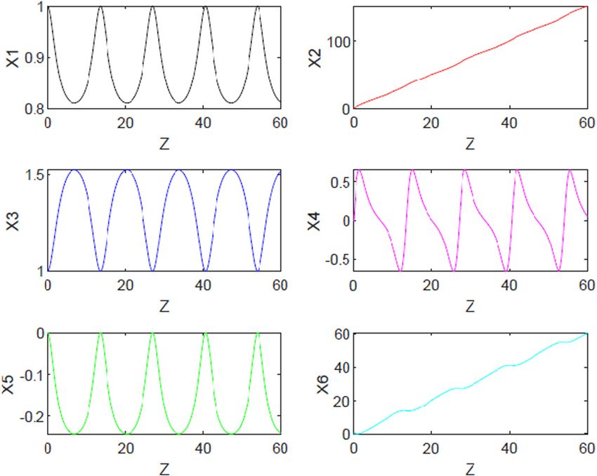
560 Reyouf Alrashed et al.
of motions are set to be numerically examined with the 2.2 Perturbed Chen–Lee–Liu (PCLL)
help of fourth-order Runge–Kutta numerical technique. equation
Moreover, different methods have been utilized in the lit-
erature to examine various forms of evolution equations The governing CLL equation in the presence of perturba-
as cited in the above references and references therein; tion terms is expressed in dimensionless as follows [13,14]:
besides, most of these methods used to examine the CLL
iqz + aqtt + ib∣q ∣2 qt = i[αqt + β (∣q∣2 q )t + γ (∣q∣2 )t q]. (2)
models gave only sets of exact soliton solutions to the
model via various analytical approaches. Clearly, equation (2) emanates from equation (1) due
However, we employ in this study the collective vari- to the presence of perturbation terms with q = q (z , t )
able method to investigate two forms of the CLL equa- being the complex-valued wave function that depends
tions. Specifically, we will examine the CCLL and the on the spatial and temporal variables z and t , respec-
PCLL equations. Also, certain graphical illustrations of tively. Similarly, the real constants a and b represent
the simulated numerical results will be depicted to the coefficients of the group-velocity dispersion and non-
portray the pulse interactions, in addition to identifying linearity term, respectively. Furthermore, going to the
the influential parameters in each model that charac- other side of the equation, the real constant α denotes
terize the evolution of pulse propagation in the media. the coefficient of inter-modal dispersion; while the real
Additionally, we arrange the present study as follows: constants β and γ denote the coefficients of self-stee-
Section 2 gives the two models of interest; while Section pening and nonlinear dispersion, respectively. Moreover,
3 gives the basic outline of the adopted methodology. the subscripts in equations (1) and (2) are partial deriva-
Section 4 considers a particular pulse configuration func- tives in the respective spatial and time variables.
tion f through the Gaussian ansatz to construct the
resulting equations of motions for both models; while
Sections 5 and 6 present the numerical results and con-
clusion, respectively. 3 Collective variable methodology
This section presents the method collective variable
approach [35–43] based on the initial work by Boesch
2 Governing equations et al. [44]. First, the method starts off by splitting the
complex-valued wave function (solution) of the given
In this section, we consider the two famous dimension- nonlinear Schrödinger equation into two parts. The first
less types of the governing CLL equation to be analyzed part constitutes the soliton solution that is called the pulse
in the present study. configuration; while the second part is called the residual
field function. Mathematically, we express the complex-
valued wave function q (z , t ) after splitting as
q (z , t ) = f (z , t ) + g (z , t ) , (3)
2.1 Classical Chen–Lee–Liu (CCLL) equation
where f (z , t ) is the pulse configuration and g (z , t ) is the
The governing CCLL equation that is known for its var- residual field function. Moreover, the pulse configuration
ious applications in optical fibers is given in dimension- function f (z , t ) is further assumed to depend on N vari-
less form as follows [8–12]: ables symbolically represented by Xj , for j = 1, 2, … , N .
Thus, the above equation in the presence of these new
iqz + aqtt + ib∣q ∣2 qt = 0, (1)
variables can be expressed as
where q = q (z , t ) is the complex-valued wave function q (z , t ) = f (X1 , X2 , … , XN , t ) + g (z , t ) , (4)
that depends on the spatial and temporal variables z
and t, respectively. Furthermore, the real constant a where the collection of these new variables stands for the
represents the coefficient of group-velocity dispersion; soliton’s amplitude, central position, inverse-width, chirp,
while b is a real constant that denotes the coefficient of frequency, and the phase among others. Additionally, the
nonlinearity. Additionally, it is very clear for one to introduction of these new variables in the pulse configura-
obtain a regular CLL equation from equation (1) by simply tion function f increases the degree of freedom, which
setting a = 1 and b = 1. results in the available phase space of the dynamical
Optical solitons via the collective variable method for the CCLL and PCLL equations 561
equations. Thus, in view of the objectionable effect, the Therefore, on using Dirac’s theory, a function is
constraints and the residual free energy expressed as nearly not zero for all parameters, if its variations can
∞ ∞ be set to zero [35–43]. Hence, Cj is minimum when
E= ∫ ∣g∣2 dt = ∫ ∣q − f (X1, X2 , … , XN , t )∣2 dt , (5) Cj ≈ 0 (10)
−∞ −∞
and
should be minimized. Now, if Cj designates the partial Ċj ≈ 0. (11)
derivative of the residual free energy with respect to
(w.r.t.) Xj , then Thus, on using either of the governing models given
∞ ∞
in equations (1) and (2), we have
∂E ∂ ∂ N
Cj =
∂Xj
=
∂Xj
∫ ∣g∣2 dt =
∂Xj
∫ gg∗dt , qz = ∑
∂f dXj
+
∂g (z , t )
, (12)
−∞ −∞ ∂Xj d z ∂z
∞ ∞ (6) j=1
∗
= ∫ ∂
∂Xj
gg ∗dt = ∫ ⎛ ∂∂Xgj g∗ + g ∂∂gXj ⎞dt.
⎜ ⎟
or equally
−∞ ⎝ ⎠ N
−∞ ∂f dXj ∂g (z , t )
∑ + = τr , r = c, p, (13)
Additionally, since j=1
∂Xj dz ∂z
g (z , t ) = q (z , t ) − f (X1(z , t ) , X2 (z , t ) , … , XN (z , t ) , t ) , (7) where r = c corresponds to the CCLL equation given in
equation (1), and r = p stands for the PCLL equation
we could rewrite equation (6) as
given in equation (2).
∂g ∗ ∂g ∗ Therefore, the CCLL equation given in equation (1)
Cj = , g + g,
∂Xj ∂Xj coupled to equation (12) reveals from equation (13) the
following:
∂g ∗ ∂g ∗
= ,g + ,g , τc = iaftt + iagtt − b∣f + g∣2 ft − b∣f + g∣2 gt . (14)
∂Xj ∂Xj
∂g ∗ ∂g ∗ Similarly, combination of the PCLL equation given in
= ,g + ,g equation (2) to equation (12) yields via equation (13) the
∂Xj ∂Xj
following:
⎛ ∂g ∗ ⎞
= 2R⎜ ,g ⎟, τp = iaftt + iagtt − b∣f + g∣2 ft − b∣f + g∣2 gt + αft
∂Xj (8)
⎝ ⎠ (15)
+ αgt + β (∣f + g∣2 f )t + β (∣f + g∣2 g )t
⎛ ∂(q (z , t ) − f (X1 , X2 , … , Xn , t ))∗ ⎞
= 2R⎜ , g ⎟, + γ (∣f + g∣2 )t ( f + g ) .
∂Xj
⎝ ⎠
Thus, we express from equation (13) the following:
⎛ ∂q∗(z , t ) ∂f ∗(X1 , X2 , … , Xn , t ) ⎞
= 2R⎜ − ,g ⎟, N
∂Xj ∂Xj ∂g ∂f dXj
⎝ ⎠ = −∑ + τr , r = c, p. (16)
∞
∂z j=1
∂Xj dz
⎛ ∂f ∗ ⎞ ⎛ ∂f ∗ ⎞
= − 2R⎜
∂Xj
, g ⎟ = − 2R⎜
⎜ ∂Xj ⎟
∫
g dt ⎟ , On putting equation (16) into equation (9), we thus obtain
⎝ ⎠ ⎝ −∞ ⎠ ∞
⎛N ∂f ∗ ∂f
N
∂ 2f ∗ ⎞ dXk
C˙ j = − 2R⎜ ∑ ⎛⎜−
∞
with ⟨.,.⟩ denoting ∫ (⋅ ) and R denotes the real part of
−∞ ⎜ k=1
∫
∂Xj ∂Xk
+ ∑ g ⎟dt
∂Xk ∂Xj ⎠ dz
the given expressions. Therefore, the rate of change of Cj ⎝ −∞ ⎝ k=1
w.r.t. z is expressed as follows: ∞
∗ ⎞
dCj
+ ∫ ∂∂fXj τr dt ⎟⎟,
C˙ j = −∞ ⎠ (17)
dz ∞
N
∂f ∗ ∂ 2f ∗ dX
∫ ⎛ ∂Xj ∂∂Xfk
∞
⎧d⎛ ∂f ∗ ⎞⎫ = 2R ∑ ⎜ − g ⎟⎞dt k
= − 2R ⎜
⎨ dz ⎜ ∂Xj
∫
g dt ⎟ ,
⎟⎬ (9) k=1
−∞ ⎝
∂Xk ∂Xj ⎠ dz
⎩ ⎝ −∞ ⎠⎭ ∞
∗
⎛
∞
∂f ∗ ∂g
N
∞
∂ 2f ∗
∂Xk ⎞ − 2R ∫ ∂∂fXj τr dt ,
= − 2R⎜
⎜
∫
∂Xj ∂z
dt + ∑ ∫ ∂Xj∂Xk ∂z
g dt ⎟ .
⎟
−∞
k=1
⎝ −∞ −∞ ⎠
for j ∈ {1, 2, 3, … , N } .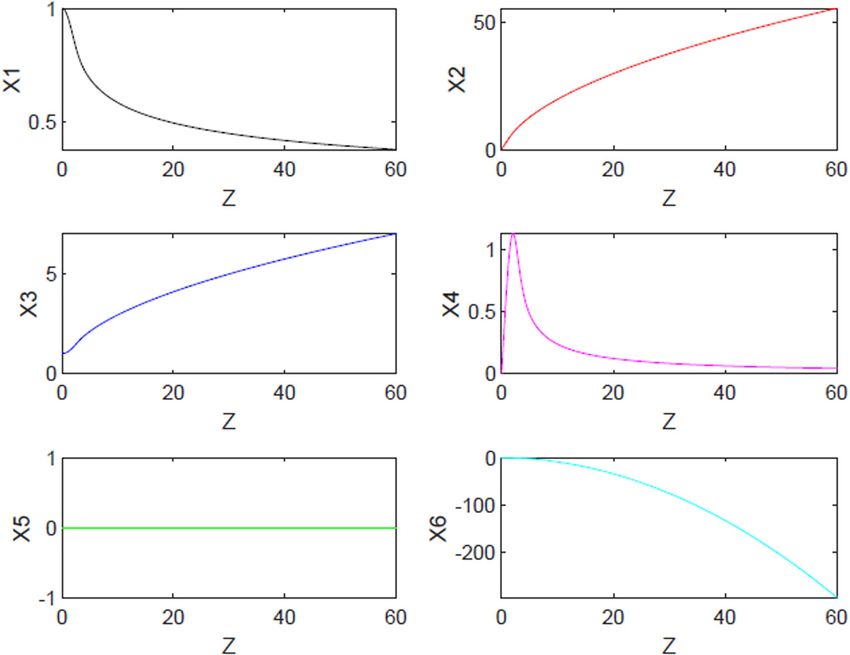
562 Reyouf Alrashed et al.
Alternatively, equation (17) can equally be expressed The equations of the collective variables otherwise
in compact form as follows: called the dynamical equations of motions are deter-
∂C ˙ mined through the application of the theory of lowest
C˙ = X + R, (18) order collective variable, also referred to as the bare
∂X
approximation (theory). Thus, with this development,
with the residual field function g (z , t ) becomes zero.
⎛ ∂C1 ∂C1
⋯
∂C1 ⎞
⎜ ∂X1 ∂X2 ∂XN ⎟
⎜ ∂C2 ∂C2 ∂C2 ⎟
∂C ⋯ 4.1 Dynamical equations of motions for CCLL
= ⎜ ∂X1 ∂X2 ∂XN ⎟,
∂X ⎜ equation
⋮ ⋮ ⋮ ⎟
⎜ ∂C ∂CN ⎟
N ∂CN
⋯ (19)
⎜ ⎟ To determine the resulting dynamical equations of motions
∂
⎝ 1X ∂X2 ∂XN ⎠
of the CCLL equation given in equation (1), we first compute
⎡ X˙ 1 ⎤ ⎡ R1 ⎤ the entries of the matrix R with the help of Maple soft-
⎢ ⎥
X˙ = ⎢ X˙ 2 ⎥, R = ⎢ R2 ⎥, ware as
⋯ ⎢⋯⎥
⎢ ⎥ ⎢ RN ⎥
X ˙
⎣ N⎦ ⎣ ⎦ R1 = 0, (22)
π x12 (2 2 ax5(3x42x34 + 4x52x32 + 12) + b(x42x34 + 8x52x32 + 4)x12 )
R2 = − , (23)
8x3
where the entries are explicitly computed using R3 = − 2π ax12x4, (24)
∞
∗ π x12x3( 2 a(3x42x34 + 4x52x32 − 4) + 2bx12x5x32 )
Rj = − 2R ∫ ∂∂fXj τr dt and R4 =
32
, (25)
−∞
(20)
∞
π x33x4(4 2 ax5x12 + bx14)
∂Ci ∗ 2 ∗
⎛⎜ ∂f ∂f − ∂ f g ⎞⎟dt . R5 = , (26)
∂Xj
= 2R ∫ 8
−∞ ⎝ ∂Xi ∂Xj ∂Xi∂Xj ⎠
π x12 ( 2 a(x42x34 + 4x52x32 + 4) + 4bx12x5x32 )
R6 = . (27)
4x3
Therefore, the resulting dynamical equations of
4 Dynamical equations of motions motions are thus given by
This section determines the resulting dynamical equa- X˙ 1 = −ax1x4, (28)
tions of motions of the two forms of CLL equations under
1
consideration via the outlined collective variable method. X˙ 2 = (8ax5 + 2 bx12 ) , (29)
4
First, by the Gaussian ansatz, we suppose the following
pulse configuration function f (X1 , X2 , X3 , X4 , X5 , X6) for X˙ 3 = 2ax3x4, (30)
both models as follows:
8a 2 bx5x12
X˙ 4 = −2ax42 + 4 + , (31)
f (X1 , X2 , X3 , X4 , X5 , X6) x3 x32
(t − X2 )2
(21)
= X1e
−
x32 ei( 2 (t − X2)
X4 2
+ X5(t − X2 ) + X6 ), Ẋ5 = 0, (32)
with the pulse characteristic parameters including the 2a 3bx5x12
X˙ 6 = ax52 − 2 − . (33)
amplitude X1, central position X2 , inverse-width X3 , chirp x3 4 2
X4 , frequency X5, and the phase X6 .Optical solitons via the collective variable method for the CCLL and PCLL equations 563
4.2 Dynamical equations of motions for CCLL [8–11] and PCLL [12,13] models. Moreover, the
PCLL equation obtained dynamical equations of motions via the appli-
cation of the collective variable method [35–43] in both
To determine the resulting dynamical equations of motions cases and given in equations (28)–(33) and equations
of the PCLL equation given in equation (2), we first compute (40)–(45), respectively, are simulated numerically for
the entries of the matrix R as follows:
R1 = 0, (34)
2 2π x12 (x42x34(α − 3ax5) + 4x52x32 (α − ax5) + 4(α − 3ax5)) π x12 (x12 ((x32x42 + 8x52 )x32 ( −(b − β )) − 4b + 8γ + 12β ))
R2 = + , (35)
8x3 8x3
R3 = −a 2π x12x4, (36)
π x12x3( 2 a(3x42x34 + 4x52x32 − 4) − 2x32x5(2 2 α + x12 (β − b)))
R4 = , (37)
32
π x12x33x4(x12 (b − β ) − 2 2 (α − 2ax5))
R5 = , (38)
8
π x12 ( 2 (4x5x32 (ax5 − α) + ax42x34 + 4a) + 4x12x5x32 (b − β ))
R6 = . (39)
4x3
Thus, the resulting dynamical equations of motions the dynamics of pulse parameters with the help of fourth-
are as follows: order Runge–Kutta numerical technique. In doing so, we
consider the following common initial conditions in both
X˙ 1 = −ax1x4, (40)
the CCLL and PCLL models as:
x 2 (b − 2γ − 3β ) X1 = X3 = 1, at t = 0, (46)
X˙ 2 = 2ax5 + α + 1 , (41)
2 2
and
X˙ 3 = 2ax3x4, (42)
X2 = X4 = X5 = X6 = 0 at t = 0. (47)
8a 2 x5x12 (b − β)
X˙ 4 = −2ax42 + 4 + , (43) More so, Figure 1 depicts the discrepancy of the pulse
x3 x32
characteristic parameters including the amplitude X1,
x 2 x 4 (γ + β ) central position X2 , inverse-width X3 , chirp X4 , frequency
X˙ 5 = − 1 , (44)
2 X5, and the phase X6 with respect to a specified distance z
of the CCLL equation; while Figures 2 and 3 give similar
2a x5x12 (3b + 4γ + β ) depictions in relation to the PCLL equation. In Figure 1,
X˙ 6 = ax52 − 2 − . (45)
x3 4 2 the influence of the pulse propagation parameters is not
that visible for different values of a and b with regards to
the CCLL equation; however, X4 seems to be an active
5 Numerical simulations and parameter in the propagation having oscillates. Also, it
is noted in Figures 2 and 3 that the pulse parameters
discussion X1 , X3 , X4 , and X5 are the most influential parameters as
the real constant b increases with regard to the evolution
In this section, we give some graphical depictions of the of pulse propagation associated with the PCLL equation
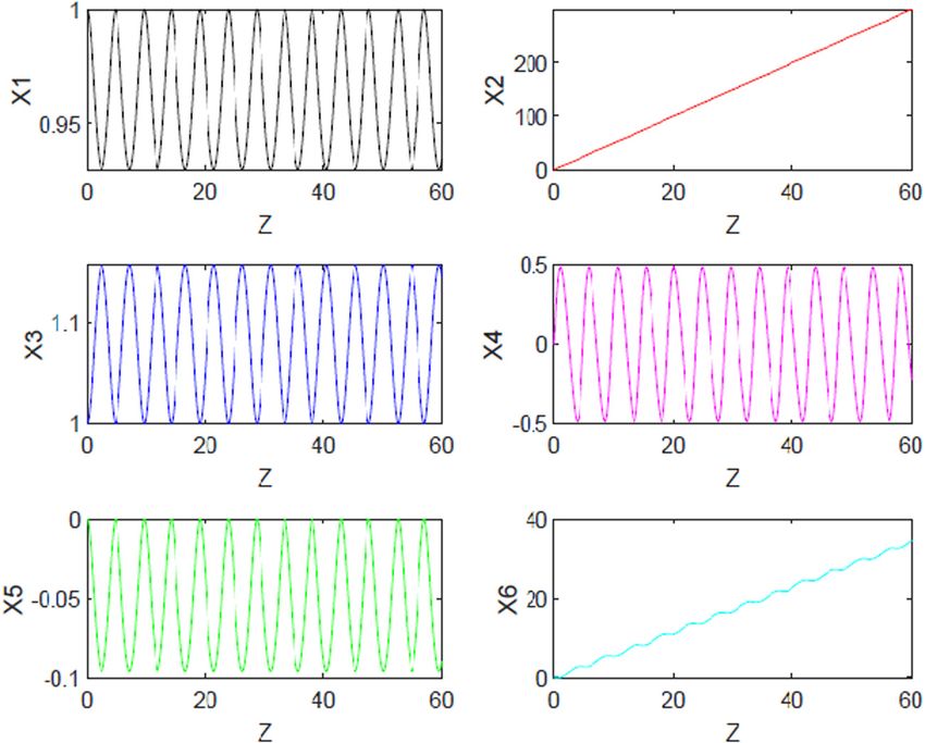
obtained computational results with regard to both the (see Figure 4 for b = 8).564 Reyouf Alrashed et al. Figure 1: Evolution of pulse characteristic parameters against the propagating distance when a = 0.1 , b = 10. Figure 2: Evolution of pulse characteristic parameters against the propagating distance when a = 0.1 , b = 9, α = 0.25, β = 0.1 , and γ = 0.1 .
Optical solitons via the collective variable method for the CCLL and PCLL equations 565
Figure 3: Evolution of pulse characteristic parameters against the propagating distance when a = 0.1 , b = 15, α = 0.25, β = 0.1 , and γ = 0.1 .
Figure 4: Evolution of pulse characteristic parameters against the propagating distance when a = 0.1 , b = 8, α = 0.25, β = 0.1 , and γ = 0.1 .
6 Conclusion equation. The method is a very powerful technique that
splits the complex-valued wave function into two com-
In conclusion, the collective variable method is employed ponents and thereafter introduces new variables to char-
to investigate the evolution of pulse propagation via acterize the dynamics of soliton propagation. Additionally,
optical solitons of the two famous members of the CLL the method is a mixture of an analytical process with a566 Reyouf Alrashed et al.
computational technique or a semi-analytical process. [10] Yildirim Y. Optical solitons to Chen–Lee–Liu model in bire-
More specifically, we extensively examined the classical fringent fibers with modified simple equation approach. Optik.
and perturbed versions of the CLL equation in optical 2019;183:612–8.
[11] Zhao Y, Fan EG. N-soliton solution for a higher-order
fibers. Also, we provided supportive graphical depictions
Chen–Lee–Liu equation with nonzero boundary conditions.
for the simulated numerical results of both models that Mod Phys Lett B. 2020;34:2050054.
depicted pulse interactions in terms of the soliton para- [12] Biswas A, Ekisi M, Sonimezoglu A, Alshomrani AS, Zhou Q,
meters. Finally, we identified the most influential para- Moshokoa SP, et al. Chirped optical solitons of Chen–Lee–Liu
meters in each model that characterized pulse propagation equation by extended trial equation scheme. Optik.
2018;156:999–1006.
in the media. In the end, it is recommended that other com-
[13] Yildirim Y, Biswas A, Asma M, Ekici M, Ntsime BP, Zayed EME,
plex-valued nonlinear evolution equations can be scruti- et al. Optical soliton perturbation with Chen–Lee–Liu equa-
nized using the employed method. tion. Optik. 2020;220:165–77.
[14] Biswas A. Chirp-free bright optical soliton perturbation with
Funding information: The authors state no funding Chen–Lee–Liu equation by traveling hypothesis and semi-
inverse variational principle. Optik. 2018;172:772–6.
involved.
[15] Aljohani AF, El-Zahar ER, Ebaid A, Ekici M, Biswas A. Optical
soliton perturbation with Fokas-Lenells model by Riccati
Author contributions: All authors have accepted respon- equation approach. Optik. 2018;172:741–5.
sibility for the entire content of this manuscript and [16] Biswas A, Kara AH, Alqahtani RT, Ullah MZ, Triki H, Belic M.
approved its submission. Conservation laws for optical solitons of Lakshmanan-
Porsezian-Daniel model. Proc Roman Acad Ser A.
2018;19(1):39–44.
Conflict of interest: The authors state no conflict of
[17] Lakshmanan M, Porsezian K, Daniel M. Effect of discreteness
interest. on the continuum limit of the Heisenberg spin chain. Phys Lett
A. 1988;133(9):483–8.
[18] Alqahtani RT, Babatin MM, Biswas A. Bright optical solitons for
Lakshmanan-Porsezian-Daniel model by semi-inverse varia-
References tional principle. Optik. 2018;154:109–14.
[19] Biswas A, Yildirim Y, Yasar E, Zhou Q, Moshokoa SP, Belic M.
[1] Liu WJ, Tian B, Zhang HQ, Li LL, Xue YS. Soliton interaction in the Optical solitons for Lakshmanan-Porsezian-Daniel model by
higher-order nonlinear Schrödinger equation investigated with modified simple equation method. Optik. 2018;160:24–32.
Hirotaas bilinear method. Phys Rev E. 2008;77(6):066605. [20] Mohammed WW, Abdelrahman MAE, Hamza AE, Akinlar MA.
[2] Sulaiman TA, Bulut H, Atas SS. Optical solitons to fractional Soliton solutions for system of ion sound and Langmuir waves.
Schrödinger-Hirota equation. Appl Math Nonl Sci. 2019;4(2):535–42. Opt Quant Electro. 2020;52:460.
[3] Xianguo G, Yanyan L. Darboux transformation for an integrable [21] Qingjie C, Tiande Z, Djidjeli K, Price DW, Twizell EH. Soliton
generalization of the nonlinear Schrödinger equation. solution of a class of generalized nonlinear Schrödinger
Nonlinear Dyn. 2012;69(4)2012:1621–30. equations. Math J Chin Univ. 1997;12(4):389–98.
[4] Nuruddeen RI. Elzaki decomposition method and its applica- [22] Seadawy AR, Khalid KA, Nuruddeen RI. A variety of soliton
tions in solving linear and nonlinear Schrödinger equations. solutions for the fractional Wazwaz-Benjamin-Bona-Mahony
Sohag J Math. 2017;4(2):31–35. equations. Results Phys. 2019;12:2234–41.
[5] Bakodah HO, Banaja MA, Alqarni AA, Alshaery AA, Younis M, [23] AlQarni AA, Banaja MA, Bakodah HO. Numerical analyses
Zhou Q, et al. Optical solitons in birefringent fibers with optical solitons in dual core couplers with Kerr law nonli-
Adomian decomposition method. J Comput Theor Nanosci. nearity. Appl Math. 2015;6:1957–67.
2015;12(10):5846–58. [24] Bakodah HO, Banaja MA, Alshaery AA, AlQarni AA. Numerical
[6] Banaja MA, AlQarni AA, Bakodah HO, Zhou Q, Moshokoa SP, solution of dispersive optical solitons with Schrödinger-Hirota
Biswas A. The investigate of optical solitons in cascaded equation by improved Adomian decomposition method.
system by improved adomian decomposition scheme. Optik. Math Probl Eng. 2019;2019:2960912.
2017;130:1107–14. [25] AlQarni AA, Ebaid A, Alshaery AA, Bakodah HO, Biswas A,
[7] Bernstein I, Zerrad E, Zhou Q, Biswas A, Melikechi N. Khan S, et al. Optical solitons for Lakshmanan-Porsezian-
Dispersive optical solitons with Schrödinger Hirota equation Daniel model by Riccati equation approach. Optik.
by traveling wave hypothesis. Optoelectron Adv Materials- 2019;128:922–9.
Rapid Commun. 2015;9(5–6):792–7. [26] Khalid KA, Nuruddeen RI, Raslan KR. New hyperbolic struc-
[8] Chen HH, Lee YC, Liu CS. Integrability of nonlinear Hamiltonian tures for the conformable time fractionalvariant bussinesq
systems by inverse scattering method. Phys Scr. equations. Opt Quant Electron. 2018;50:1–10.
1979;20:490–2. [27] Sedeeg AKH, Nuruddeen RI, Gomez-Aguilar JF. Generalized
[9] Bansal A, Biswas A, Zhou Q, Arshed S, Alzahrani AK, Belic MR. optical soliton solutions to the (3.1) dimensional resonant
Optical solitons with Chen–Lee–Liu equation by Lie symmetry. nonlinear Schrödinger equation with Kerr and parabolic law
Phy Let A. 2020;384(10):126202. nonlinearities. Opt Quant Electro. 2019;51:173.Optical solitons via the collective variable method for the CCLL and PCLL equations 567
[28] Biswas A, Ekici M, Sonmezoglu A, Triki H, Majid FB, Zhou Q, [36] Green P, Milovic D, Lott D, Biswas A. Dynamics of Gaussian
et al. Optical solitons with Lakshmanan-Porsezian-Daniel optical solitons by collective variables method. Appl Math
model using a couple of integration schemes. Optik. Infor Sci. 2008;2:259–73.
2018;158:705–11. [37] Asma M, Othman W, Wong B, Biswas A. Chirped optical
[29] Nuruddeen RI, Nass AM. Exact solitary wave solution for the Gausson perturbation with quadratic-cubic nonlinearity by
fractional and classical GEW-Burgers equations: an applica- collective variables. Opt Quant Electron. 2019;51:200.
tion of Kudryashov method. J Taibah Univ Sci. [38] Veljkovic M, Milovic D, Belic M, Zhou Q, Moshokoa SP,
2018;12(3):309–14. Biswas A. Super-sech soliton dynamics in optical metamater-
[30] Islam MT, Akbar MA, Azad AK. Multiple closed form solutions ials using collective variables. Facta Univ Ser Electron Energ.
to the KdV and modified KdV equations through the rational 2017;30:39–48.
(G/G)-expansion method. J Asso Arab Univ Basic Appl Sci. [39] Moubissi AB, Dinda PT, Kofane TC. Note on collective variable
2017;24:160–8. theory of nonlinear Schrödinger solitons. J Phy A Math
[31] Yıldırım Y. Optical solitons to Chen–Lee–Liu model with trial General. 2000;33(12):2453.
equation approach. Optik. 2019;183:849–53. [40] Moubissi AB, Nakkeeran K, Dinda PT, Kofane TC. Non-
[32] Yıldırım Y, Dakova A, Biswas A, Khan S, Moshokoa SP, Lagrangian collective variable approach for optical solitons in
Alzahrani AK, et al. Cubic-quartic optical soliton perturbation fibres. J Phy A Math General. 2001;34(1):129.
with Fokas-Lenells equation by sine-Gordon equation [41] Shwetanshumala S. Temporal solitons in nonlinear media
approach. Results Phy. 2021;26:104409. modeled by modified complex Ginzburg Landau equation under
[33] Triki H, Benlalli A, Zhou Q, Biswas A, Yıldırım Y, Alzahrani AK, collective variable approach. Int J Theor Phy. 2009;48(4):1122.
et al. Gray optical dips of Kundu-Mukherjee-Naskar model. [42] Biyoghe S, Ekogo TB, Moubissi AB. Collective variable ana-
Phy Lett A. 2021;401(17):127341. lysis of the nonlinear Schrödinger equation for soliton
[34] Yıldırım Y, Biswas A, Kara AH, Ekici M, Zayed EM, Alzahrani AK, molecules in fibers. J Nonlinear Opt Phy Mater.
et al. Cubic-quartic optical soliton perturbation and conser- 2017;26(2):1750023.
vation laws with Kudryashovas law of refractive index. [43] Olivier A, Diby A, Yoboue P, Kamagate A. Spatio-temporal
Phy Lett A. 2020;384(34):126884. pulsating dissipative Solitons through collective variable
[35] Veljkovic M, Xu Y, Milovic D, Mahmood MF, Biswas A, Belic MR. methods. J Appl Math Phy. 2016;4:1032–41.
Super-Gaussian solitons in optical metamaterials using [44] Boesch R, Stancioff P, Willis CR. Hamiltonian equations for
collective variables. J Comput Theor Nanosci. multiple-collective-variable theories of nonlinear Klein-
2015;1:5119–24. Gordon equations. Phy Rev B. 1988;38(10):6713–35.You can also read