Fast 4D Segmentation of Large Datasets using Graph Cuts

Fast 4D Segmentation of Large Datasets using Graph Cuts
                        Herve Lombaerta , Yiyong Sunb , and Farida Cherieta
                   a École   Polytechnique de Montréal, Montréal, Québec, Canada
                      b Siemens    Corporate Research, Princeton, NJ 08540, USA

                                               ABSTRACT
In this paper, we propose to use 4D graph cuts for the segmentation of large spatio-temporal (4D) datasets.
Indeed, as 4D datasets grow in popularity in many clinical areas, so will the demand for efficient general seg-
mentation algorithms. The graph cuts method1 has become a leading method for complex 2D and 3D image
segmentation in many applications. Despite a few attempts2–5 in 4D, the use of graph cuts on typical medical
volume quickly exceeds today’s computer capacities. Among all existing graph cuts based methods6–10 the mul-
tilevel banded graph cuts9 is the fastest and uses the least amount of memory. Nevertheless, this method has
its limitation. Memory becomes an issue when using large 4D volume sequences, and small structures become
hardly recoverable when using narrow bands. We thus improve the boundary refinement efficiency by using a 4D
competitive region growing. First, we construct a coarse graph at a low resolution with strong temporal links to
prevent the shrink bias inherent to the graph cuts method. Second, we use a competitive region growing using
a priority queue to capture all fine details. Leaks are prevented by constraining the competitive region growing
within a banded region and by adding a viscosity term. This strategy yields results comparable to the multilevel
banded graph cuts but is faster and allows its application to large 4D datasets. We applied our method on both
cardiac 4D MRI and 4D CT datasets with promising results.

                                          1. INTRODUCTION
The amount of information contained in medical images can become overwhelming during an intervention,
especially when dealing with volume sequences. The time spent in interpreting these images can be greatly
decreased with segmentation algorithms, highlighting anatomical structures of interest, thus leading to a better
image understanding and organ localization. Spatial images (2D and 3D) have been heavily studied. Spatio-
temporal images (4D, or 3D+t) are becoming widely available and they still present an unsolved computational
challenge. Scanners output gigabytes of data and the trend is towards even higher definitions.
    Explicit deformable models11, 12 have been used as initial attempts for 4D segmentation. Free form deforma-
tions11 and simplex meshes12 have been applied in the temporal domain to track 3D surfaces over time. However,
4D segmentation is not treated as a whole; the temporal dimension is rather treated separately. The surface of
a particular frame serves as an initial guess for the next frame. Later, temporal correlation13 is considered by
adding 4D a priori knowledge in the segmentation. A probabilistic 4D atlas14 can help the segmentation using
the EM algorithm, and temporal constraints15 can also be incorporated in a 4D deformable model. The level
set method16 is a well established segmentation algorithm in 2D and 3D images. Although this method is easily
extendable to N -D, few works have been done in 4D. For instance, a 4D levelset17 is used to approximate the
aortic shape, the surface itself is computed with a graph-based method. Shape priors are used18, 19 to improve
the segmentation of low quality images. The Graph Cuts method20 uses the maxflow algorithm to find the min-
imum cut on a graph. Compared with the previous local approaches, maxflow-mincut algorithms yield optimal
solutions in polynomial time. Graph Cuts have already been used for 4D surface selection2 and reconstruction.21
In image segmentation, although being N -D interactive, Boykov and Jolly’s method1 is impractical for typical
4D medical datasets using current processing capacities. New designs have been proposed to get around this
issue. Active contours6 are simulated by evolving banded graph cuts. However, in this method, the band inner
boundary has a smaller surface than the band outer boundary; the difference in surface area creates a shrinkage
bias. Lazy snapping7, 22 uses the graph cuts technique on watershed regions of the image. The algorithm pre-
segmentation is however time consuming when using large datasets, and produces an unpredictable number of
watershed regions. Moreover, the fine segmentation depends on the watershed boundaries, and as shown in,23
these boundaries are not necessarily robust to noise. Rather than watershed regions, the mean shift algorithm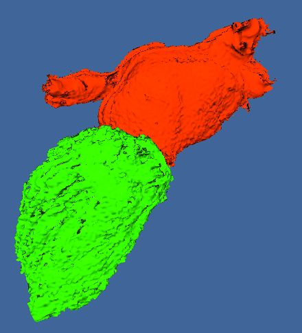

Figure 1. 4D graph corresponding to 3 frames of a 33 volume. Spatial n-links in grey lines, temporal n-links for a single
node in green lines, and t-links in red and blue.

has been used8 to segment objects in a (2D+t) video. This method still relies on pre-segmented results, which
are also time-consuming in this case. A different coarse-to-fine approach is the multilevel banded graph cuts
method.9 The algorithm iteratively projects the results from a coarse image up to the fine resolution. Results in
2D and 3D are comparable to the standard graph cut algorithm. However, small and thin structures can easily
be lost with this method when using very large 4D datasets. Active Graph Cuts10 could solve this problem as it
retains the global optimality of the solution, but requires the same amount of memory than the standard graph
cuts. Laplacian pyramids24 could be used in order to catch finer details. These graph cuts based techniques are
all efficient with 2D and 3D images, but the memory required by large 4D datasets is prohibitive.
   We propose in section 2 a segmentation method based on 4D graph cuts. To overcome the computational
limitation, a coarse-to-fine strategy is developed. Results presented in section 3 show that the segmentation
accuracy is indeed improved when using 4D graph cuts rather than when using 3D graph cuts sequentially.
Moreover, our method performs well in segmentation of cardiac structures on both 4D MR and 4D CT. A
general discussion as well as guidelines for future work are provided in section 4.

                                                    2. METHOD
First, the graph cuts algorithm for image segmentation20 is briefly described. In a graph representing a 4D
image, a cut separates graph nodes into two categories, object and background. Second,a coarse-to-fine strategy
is developed in order to successfully run the method on large 4D datasets.

2.1 4D Graph Cuts
Given a 4D image, a weighted undirected graph G = hV, Ei is constructed (Fig. 1). There are two special nodes,
or vertices, in V, a source node specifying the “object” terminal, and a sink node specifying the “background”
terminal. Each remaining node in V uniquely identifies an image point. There are two types of edges in E,
n-links (spatial and temporal neighborhood links), and t-links (terminal links). Each image node has two t-links
connecting the node to the terminals. The n-links are determined by a spatio-temporal neighborhood system
N , e.g., |N (t) | = 26 and |N (t−1) | = |N (t+1) | = 6. The weight used for edges between two nodes p and q is
based on the data intensity difference. Boykov and Jolly1 proposed to use the weight for spatial n-links as
                                      x2
wp,q = f (|Ip − Iq |) with f (x) = e− σ2 where σ is a smoothness parameter. We define the weight of temporal n-
links as wp(t) ,q(t+1) = τ · f (|Ip(t) − Iq(t+1) |), where τ is a parameter implementing temporal integrity. Additionally,
the user provides the seed points O and B marked as “object” and “background” (Fig. 2(a)). The t-links of
these seed points have infinity weights, i.e., wp,”obj” = ∞|p ∈ O, and wp,”bkg” = ∞|p ∈ B. Zero weight t-links
are used elsewhere. The segmentation is determined by a cut C on the graph. Severed edges in E separate the
terminal nodes, classifying    P each image node into either object or background. The cost of a cut is the sum of
all severed edges: |C| = ep,q ∈C wp,q . Therefore, segmentation can be solved by finding the minimum cut on
the graph. This can be computed efficiently with polynomial-time complexity algorithms such as Boykov and
Kolmogorov’s maxflow implementation.20
   The graph cuts method is known25 to have a bias towards small cuts. The cost of a small cut surrounding
the seed points might be cheaper than the cost of a larger cut around the object’s boundary. In 4D, it might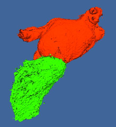

Figure 2. Banded approach: (a) object and background seed points provided by the user; (b) global shape computed
via graph cuts; (c) construction of the band around the coarse boundary; (d) refinement of the boundary (thick black
contour) using fast competitive region growing.

be cheaper to segment the organ in a single 3D frame rather than in the whole 4D sequence. We propose to
use slightly more expensive temporal n-links. When the object is assumed to be seen on all frames, stronger
temporal correlation are imposed with τ > 1.

2.2 Fast Banded Approach
For typical medical datasets, a 4D graph needs a prohibitive amount of memory. For example, the maxflow
implementation from Boykov and Kolmogorov20 requires 24|V| + 14|E| bytes. That is over 21GB for a 4D
10 × 2563 dataset. Furthermore, the polynomial complexity of the algorithm makes graph cuts impractical using
today’s processing power. To overcome this problem, the graph is constructed at a low resolution. The 4D
data is scaled down by a factor k using the mean filter, so the resulting graph fits in the computer’s memory.
Similarly, the seed point coordinates are scaled down by the factor k. Note that this factor can be different for
each dimension (e.g., k > 1 for spatial dimensions and k = 1 for the temporal dimension).
     The segmentation resulting from the low resolution graph is refined in a band around the graph’s minimum
cut (Fig. 2(c)). The band radius is ideally the size of one low resolution voxel, or k voxels in high resolution. It
is assumed that the inner surface of the band remains inside the object, and that the outer band remains outside
it. The boundary is refined using competitive region growing between the inner and the outer surfaces within
the band. Leaking, inherent to region growing algorithms, is thus confined in the band. Note that the boundary
refinement takes place in 4D, a hyper-band and hyper-regions are indeed used. Similarly to the seeded region
growing,23 all potentially new object or background voxels are placed in one priority queue. Their order in the
queue depends on the intensity difference diff (p) = |Ip − Ipar (p) | between the candidate voxel p and its parent
par (p). For a newly inserted voxel in the priority queue, its key value key(p) is an integration of previous keys,
i.e., key(p) = diff (p) + λ · key(par (p)), with λ bounded between 0 and 1. Regions first grow to include voxels
with similar intensities. However, when λ > 0, this heuristics favors the growing of regions close to the seed
points. Hence, λ simulates the smoothness of the grown boundary. In the section 3.2, a comparison between the
multilevel banded graph cuts9 and this competitive region growing shows that both methods yield comparable
results.
    Optionally, the refinement step can be iterative. During an iteration, a new band is constructed around the
previous refined boundary. This band evolution allows an incremental segmentation of structures not fully present
in the initial band (e.g., vessels originating, or ending, in the segmented organ). However, as the competitive
region growing does not yield a global optimum result, there is no guarantee of convergence to such an iterative
approach.

                                                 3. RESULTS
The method is compared with the standard graph cuts. The results, although slightly different, show that this
new method is a valid alternative when using very large 4D datasets. Segmentations of cardiac structures on
both 4D MR and 4D CT are presented.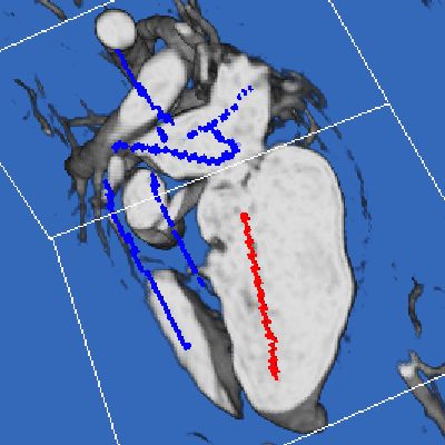

(a) ground truth              (b) noisy image                (c) 3D slice                 (d) 4D slice
Figure 3. 4D vs. 3D Segmentation with Graph Cuts: (a) ground truth with seed points, (b) image with noise, (c) slice
from the 3D segmentation (12.89% error with the ground truth), (d) slice from the 4D segmentation (7.35% error with
the ground truth).

3.1 4D vs. 3D Segmentation with Graph Cuts
Temporal correlations improves the segmentation accuracy. It is demonstrated with a noisy synthetic image where
a ground truth is known. The segmentation accuracy is compared when using the algorithm in a 3D version and
in a 4D version. The 4D volume (5 × 323 ) has a static bright cube of intensity 0.75 on a dark background of
intensity 0.25 (Fig. 3(a)). A Gaussian noise with σ = 0.35 is added to the image. With such a strong noise, spatial
information becomes weak (Fig. 3(b)). A 3D segmentation of a single 3D frame yields 12.89% of error compared
to the ground truth; 0.59% of the voxels are over-segmented, and 12.30% are under-segmented (Fig. 3(c)). When
temporal information is added in a 4D graph (|N (t) | = 26, |N (t−1) | = |N (t+1) | = 6), the segmentation error drops
to 7.35%; 0.98% of the voxels are over-segmented, and 6.37% of the voxels are under-segmented (Fig. 3(d)).

3.2 Fast 4D Segmentation
In order to measure the computational improvement of our method, a single frame from a 15 × 192 × 192 × 80
MR volume is used (Fig. 4(a)). With a core 2 duo 2.8GHz and 2GB of memory, the standard graph cuts runs
in 20.88s, and requires 1270MB of memory (Fig. 4(b)). With one level using a downscaling factor k = 5, the
multilevel banded graph cuts runs in 1.53s, and requires 47.5MB of memory. Our method runs in 0.59s and
requires 13.6MB of memory.
    When considering the whole sequence (15 frames), 23GB of memory would be required to construct a standard
4D graph. This is not possible with current computers. Since there is no ground truth available for the left
ventricle segmentation, our method is compared with the multilevel banded graph cuts. The latter runs in 44.72s,
and requires 854MB (Fig. 4(c)). With the same conditions, our method runs in 9.42s, and requires 253MB;
3.46% of the voxels are under-segmented, and 5.52% of the voxels are over-segmented (Fig. 4(d)). After a second
iteration of the boundary refinement, the error drops to 3.62% of under-segmented and 4.45% of over-segmented

       (a) seed points            (b) 3D Graph Cuts          (c) 4D M. banded GC              (d) our method
Figure 4. Comparison with existing methods: (a) seed points for the left ventricle segmentation, (b) 3D standard graph
cuts on a single frame (20.88s, 1270MB), (c) 4D multilevel banded graph cuts on 15 frames (44.72s, 854MB), (d) our
method on 15 frames (9.42sec, 253MB).

frame 1                       frame 5                      frame 9                      frame 14
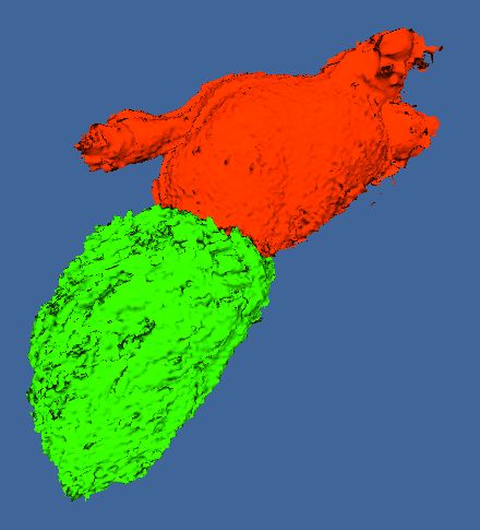
Figure 5. 4D MR Segmentation of the Left Atrium in red (10.50s, 253MB), of the Left Ventricle in green (9.51s, 253MB),
of the Right Atrium in blue (9.51s, 253MB), and of the Right Ventricle in yellow (10.83s, 253MB) from a 15×192×192×80
data.

voxels. It is possible to see differences between the multilevel banded graph cuts and our method in regions with
weak boundaries, for instance, between the left ventricle and the left atrium.

3.3 Segmentation of Cardiac Structures
From the 4D MR dataset, all 4 cardiac chambers are segmented (Fig. 5 shows the left atrium segmented in
10.50s, 253.8MB; left ventricle, 9.51s, 253.8MB; right atrium, 8.92s, 253.8MB; right ventricle, 10.83s, 253.8MB).
On even larger 4D datasets, the multilevel banded graph cuts runs out of memory. Multilevels can be used at
the expense of computation time. It is also possible to foresee the memory problem with very large datasets.
Our method runs successfully on these large datasets. Cardiac structures of a human heart are segmented in a
10 × 512 × 512 × 141 CT sequence (Fig. 6). To segment the left atrium, 79.42s and 1367MB is required. Details of
the algorithm show that the low resolution graph cuts used as little as 4.86s, and the competitive region growing
runs in 21.58s. Much of the computation time is spent constructing the band (30sec) as well as scaling down
and scaling up the volume (10sec each). To segment the left ventricle, 81.20s and 1371MB is required.

                frame 1                                 frame 4                                 frame 9
Figure 6. 4D CT Segmentation of the Left Atrium in red (79.42s, 1367MB), of the Left Ventricle in green (81.20s, 1371MB)
from a 10 × 512 × 512 × 141 data.

4. CONCLUSIONS
In this paper, 4D graph cuts have been proposed for 4D segmentation. The results showed that temporal
correlation improves the segmentation accuracy of very noisy data. In order to use graph cuts in typical medical
volumes, a coarse-to-fine strategy has been developed. In our proposed method, which is applicable to both 3D
and 4D, we improved the boundary refinement using competitive region growing. Besides yielding comparable
results, our approach is faster and uses less memory than the multilevel banded graph cuts. It is therefore well
suited for applications with very large 4D datasets. Our method shows promising results with the segmentation
of both 4D MR and 4D CT.
    Drawbacks of our method are inherent to the graph cut method. The seed size is important. If it is small,
a small graph cut around the seeds can be cheaper than a larger graph cut around the organ. In 4D datasets,
it might be cheaper to cut the organ within a single 3D frame rather than in all frames. This is usually solved
by using large seeds. To prevent these small cuts, we propose to use heavier weights for temporal links between
frames. Future work will further investigate this issue.

Acknowledgement
The authors wish to acknowledge the financial support from Siemens Corporate Research (SCR) and the Natural
Sciences and Engineering Research Council of Canada (NSERC).

                                              REFERENCES
 [1] Boykov, Y. and Jolly, M.-P., “Interactive Organ Segmentation Using Graph Cuts,” in [MICCAI], 276–286
     (2000).
 [2] Waschbüsch, M., Würmlin, S., and Gross, M., “Interactive 3D video editing,” Visual Computer 22(9),
     631–641 (2006).
 [3] Bai, X., Wang, J., Simons, D., and Sapiro, G., “Video snapcut: robust video object cutout using localized
     classifiers,” in [SIGGRAPH ], 1–11 (2009).
 [4] Vaudrey, T., Gruber, D., Wedel, A., and Klappstein, J., “Space-time multi-resolution banded graph-cut for
     fast segmentation,” in [DAGM Symposium Pattern Recognition], 203–213 (2008).
 [5] Lombaert, H. and Cheriet, F., “Spatio-temporal segmentation of the heart in 4d mri images using graph
     cuts with motion cues,” in [ISBI], (2010).
 [6] Xu, N., Bansal, R., and Ahuja, N., “Object segmentation using graph cuts based active contours,” in
     [CVPR ], 46–53 (2003).
 [7] Li, Y., Sun, J., Tang, C.-K., and Shum, H.-Y., “Lazy snapping,” in [SIGGRAPH ], 303–308 (2004).
 [8] Wang, J., Bhat, P., Colburn, A. R., Agrawala, M., and Cohen, M. F., “Interactive video cutout,” in
     [SIGGRAPH ], 585–594 (2005).
 [9] Lombaert, H., Sun, Y., Grady, L., and Xu, C., “A Multilevel Banded Graph Cuts Method for Fast Image
     Segmentation,” in [ICCV], 259–265 (2005).
[10] Juan, O. and Boykov, Y., “Active Graph Cuts,” in [CVPR ], 1023–1029 (2006).
[11] Bardinet, E., Cohen, L. D., and Ayache, N., “Tracking and motion analysis of the left ventricle with
     deformable superquadrics.,” Medical Image Analysis 1(2), 129–149 (1996).
[12] McInerney, T. and Terzopoulos, D., “A dynamic finite element surface model for segmentation and tracking
     in multidimensional medical images with application to cardiac 4D image analysis,” Computerized Medical
     Imaging and Graphics 19(1), 69–83 (1995).
[13] Chandrashekara, R., Rao, A., Sanchez-Ortiz, G. I., Mohiaddin, R. H., and Rueckert, D., “Construction of
     a Statistical Model for Cardiac Motion Analysis Using Nonrigid Image Registration,” in [IPMI], 599–610
     (2003).
[14] Lorenzo-Valdés, M., Sanchez-Ortiz, G. I., Mohiaddin, R., and Rueckert, D., “Segmentation of 4D Cardiac
     MR Images Using a Probabilistic Atlas and the EM Algorithm,” in [MICCAI], 440–450 (2003).
[15] Montagnat, J. and Delingette, H., “4D deformable models with temporal constraints: application to 4D
     cardiac image segmentation.,” Medical Image Analysis 9(1), 87–100 (2005).

[16] Osher, S. and Sethian, J. A., “Fronts Propagating with Curvature-Dependent Speed: Algorithms Based on
     Hamilton-Jacobi Formulations,” Computational Physics 79, 12–49 (1988).
[17] Zhao, F., Zhang, H., Wahle, A., Scholz, T. D., and Sonka, M., “Automated 4d segmentation of aortic
     magnetic resonance images,” in [BMVC ], 247–257 (2006).
[18] Kohlberger, T., Cremers, D., Rousson, M., Ramaraj, R., and Funka-Lea, G., “4D Shape Priors for a Level
     Set Segmentation of the Left Myocardium in SPECT Sequences,” in [MICCAI], 92–100 (2006).
[19] Abufadel, A., Yezzi, T., and Schafer, R., “4D segmentation of cardiac data using active surfaces with
     spatiotemporal shape priors,” in [SPIE ], (2007).
[20] Boykov, Y. and Kolmogorov, V., “An experimental comparison of min-cut/max-flow algorithms for energy
     minimization in vision.,” PAMI 26(9), 1124–1137 (2004).
[21] Yu, T., Xu, N., and Ahuja, N., “Reconstructing a Dynamic Surface from Video Sequences Using Graph
     Cuts in 4D Space-Time,” in [ICPR], 245–248 (2004).
[22] Li, Y., Sun, J., and Shum, H.-Y., “Video object cut and paste,” in [SIGGRAPH ], 595–600 (2005).
[23] Adams, R. and Bischof, L., “Seeded region growing,” PAMI 16(6), 641–647 (1994).
[24] Sinop, A. K. and Grady, L., “Accurate banded graph cut segmentation of thin structures using laplacian
     pyramids.,” in [MICCAI], 896–903 (2006).
[25] Shi, J. and Malik, J., “Normalized cuts and image segmentation,” PAMI 22(8), 888–905 (2000).