On the optical solutions to nonlinear Schrödinger equation with second-order spatiotemporal dispersion
←
→
Page content transcription
If your browser does not render page correctly, please read the page content below

Open Physics 2021; 19: 111–118
Research Article
Hadi Rezazadeh, Waleed Adel, Mostafa Eslami, Kalim U. Tariq,
Seyed Mehdi Mirhosseini-Alizamini, Ahmet Bekir, and Yu-Ming Chu*
On the optical solutions to nonlinear Schrödinger
equation with second-order spatiotemporal
dispersion
https://doi.org/10.1515/phys-2021-0013
received November 22, 2020; accepted February 16, 2021
1 Introduction
Abstract: In this article, the sine-Gordon expansion method The nonlinear Schrödinger equation (NLSE) is one of the
is employed to find some new traveling wave solutions to most powerful generic family of models, fascinating great
the nonlinear Schrödinger equation with the coefficients of attention of both mathematicians and physicists because
both group velocity dispersion and second-order spatio- of their potential applications in the recent era of the
temporal dispersion. The nonlinear model is reduced to optical theory. A lot of natural complex phenomena can
an ordinary differential equation by introducing an intelli- be described by this model of the nonlinear type. A good
gible wave transformation. A set of new exact solutions are understanding of the solutions, configurations, inter-
observed corresponding to various parameters. These novel dependence, and supplementary features may contribute
soliton solutions are depicted in figures, revealing the new to a more study of more complex models in several areas
physical behavior of the acquired solutions. The method of science and engineering. For example, electromagnetic
proves its ability to provide good new approximate solu- theory, condensed matter physics, acoustics, cosmology,
tions with some applications in science. Moreover, the asso- and plasma physics are some of the areas that benefit
ciated solution of the presented method can be extended to from studying this type of equation. With these above-
solve more complex models. mentioned applications, the need to further study the
Keywords: solitary wave, Schrödinger equation, sine- NLSE is of interest and this was the motivation to inves-
Gordon expansion method tigate more about the behavior of this model. The study
with an effective method which may provide accurate
results with physical meaning is an ongoing research
for such model and similar ones. In the sense of fractional
calculus, an extended model of the NLSE can be proposed
* Corresponding author: Yu-Ming Chu, Department of Mathematics, and studied to take into account the effect of the frac-
Huzhou University, Huzhou 313000, China; Hunan Provincial Key tional term. Fractional calculus has a great amount of
Laboratory of Mathematical Modeling and Analysis in Engineering,
work for solving models with applications and continues
Changsha University of Science and Technology, Changsha 410114,
China, e-mail: chuyuming2005@126.com
to prove the ability to provide more realistic models. For
Hadi Rezazadeh: Faculty of Engineering Technology, Amol example, optimal control of diabetes [1], blood ethanol
University of Special Modern Technological, Amol, Iran concentration system modeling [2], and dengue fever
Waleed Adel: Department of Mathematical Sciences, Faculty of modeling [3] are some of the real-life applications of
Engineering, Mansoura University Mansoura, Egypt
models with fractional derivatives. We are interested in
Mostafa Eslami: Department of Mathematics, Faculty of
Mathematical Sciences, University of Mazandaran, Babolsar, Iran
the future to simulate the fractional NLSE. For more
Kalim U. Tariq: School of Mathematics and Statistics, Huazhong details regarding other areas of application, one may
University of Science and Technology, Wuhan 430074, China; see refs. [4–30].
Department of Mathematics, Mirpur University of Science and Many researchers were interested in nonlinear models
Technology, Mirpur (AJK)10250, Pakistan due to their complexity. Analytical solutions can elucidate
Seyed Mehdi Mirhosseini-Alizamini: Department of Mathematics,
the physical behavior of a natural system more accurately
Payame Noor University, Tehran 19395-3697, Iran
Ahmet Bekir: Neighbourhood of Akcaglan, Imarli Street, Number: corresponding to a particular process. New, innovative,
28/4, 26030, Eskisehir, Turkey and accurate techniques are being developed to find a
Open Access. © 2021 Hadi Rezazadeh et al., published by De Gruyter. This work is licensed under the Creative Commons Attribution 4.0
International License.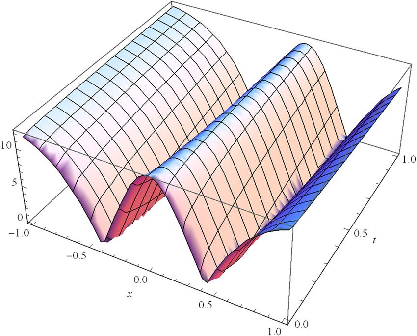
112 Hadi Rezazadeh et al.
new solution to nonlinear equations, which may contri- 2 sine-Gordon expansion method
bute in recent areas of science and technology. Recently,
many numerical and analytical approaches are being devel- The main steps of the sine-Gordon expansion method are
oped such as the auxiliary equation method [31], Cole-Hopf described below to determine an exact solution for the
transformation, exp-function method [32], sine-cosine partial differential equation. The sine-Gordon equation
method [33], Darboux transformation [34], Hirota method can take the following form [48,54]:
[35], Lie group analysis [36], modified simple equation
uxx − utt = m2 sin(u), (2)
method [37], similarity reduced method, tanh method,
inverse scattering scheme [38], Bäcklund transform method where u = u(x , t ) and m is a constant. Next, equation (2)
[39], homogeneous balance scheme [40], sine-cosine can be reduced into a nonlinear ordinary differential
method, tanh-coth method, extended FAN sub-equation equation with the aid of a traveling wave transform
method [41], auxiliary equation method [42], and many more. u(x , t ) = U (ξ ), ξ = x − νt into the following:
One of these important and effective methods that m2
may provide good solutions with important physical U″ = sin(U ), (3)
1 − ν2
behaviors is the sine-Gordon expansion method. The
method has been used numerous times for solving dif- where ν is the wave velocity in the aforementioned wave
ferent science and engineering models of physical impor- transform. Then, by multiplying both sides of equation
tance. For example, Baskonus in ref. [43] applied this (3) with the term U ′ and integrating one, we reach the
method for investigating the behavior of a Davey– following:
Stewartson equation with power-law nonlinearity, which 2
U ′
sin2 + C ,
m2 U
has some applications in fluid dynamics. Also, Yel et al. = (4)
2
2 1 − ν 2
[44] adopted the same method for solving the new
coupled Konno–Oono equation acquiring new solitons where C is an integration constant. Assuming that C = 0,
like solutions. In ref. [45], the method is used to find U m2
= H (ξ ), and 1 − ν 2 = a2 in equation (4), we obtain
2
new dark-bright solitons for the shallow water wave model.
H ′ = a sin(H ), (5)
Other related models that have been solved using this
method including Fokas–Lenells equation [46], nona- and by replacing the coefficient a = 1 into equation (5),
utonomous NLSEs equations [47], conformable time- we acquire the following equation:
fractional equations in RLW-class [48], 2D complex
H ′ = sin(H ). (6)
Ginzburg–Landau equation [49], time-fractional Fitzhugh–
Nagumo equation [50], and references therein. It is worth As can be seen, equation (6) can be considered as the
mentioning that this study is the first to be dealing with known sine-Gordon equation with a simplified form.
finding the solution to the Schrödinger equation with the Now, to solve equation (6), we adapt the separation of
coefficients of both group velocity dispersion and second- variables method and with some simplifications, one can
order spatiotemporal dispersion using this method. find the following relations:
In the present article, we use the sine-Gordon expan- sin(H (ξ )) = sech(ξ ), cos(H (ξ )) = tanh(ξ ), (7)
sion method to derive exact traveling wave solutions for
the NLSE with its coefficients of both group velocity and sin(H (ξ )) = i csch(ξ ), cos(H (ξ )) = coth(ξ ). (8)
spatiotemporal dispersion. The model can take the fol- Now, consider a nonlinear partial differential equation as
lowing form: follows:
∂q ∂q ∂ 2q ∂ 2q P(u , ux , ut , uxx , uxt , utt , …) = 0, (9)
i + α + β 2 + γ 2 + ∣q∣2 q = 0, (1)
∂x ∂t ∂t ∂x
by using the transformation u(x , t ) = U (ξ ) with ξ = x − νt ,
where q(x , t ), α, β , and γ are defined in refs. [51–53]. equation (8) can be converted into the following form:
This article is organized as follows. In Section 2, we
G(U , U ′ , U ″ , …) = 0. (10)
describe the sine-Gordon expansion method. The appli-
cation of the method is presented in Section 3. The con- The trial solution to equation (9) is assumed to be of the
clusions are drawn in Section 4. following form: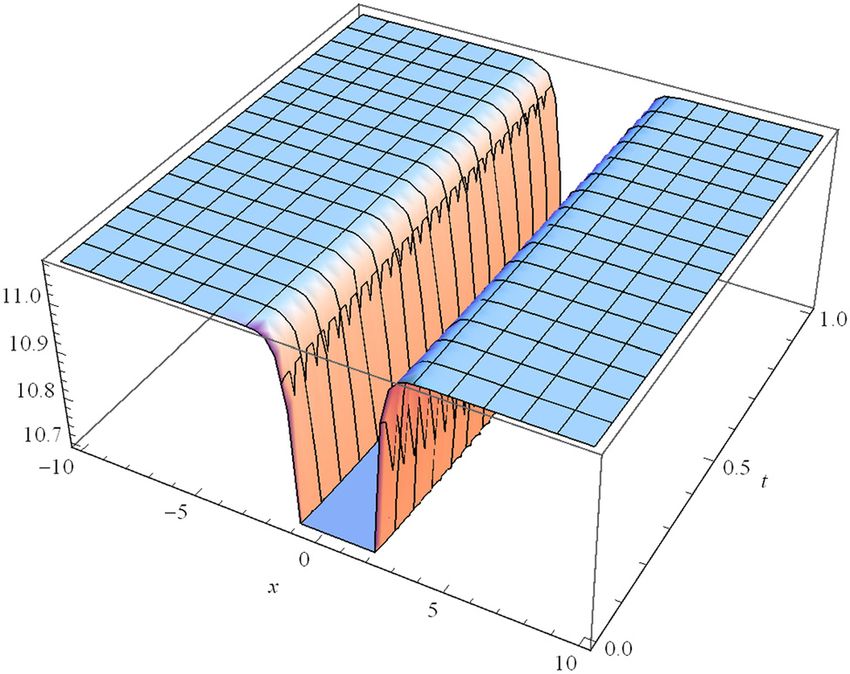
On the optical solutions to NLSE with second-order spatiotemporal dispersion 113
N
Substituting equation (14) into equation (1), we have
U (H ) = ∑ cos j−1(ξ )[Bj sin(H ) + Aj cos(H )] + A0 . (11)
j=1 i(1 − αν ) U ′ − (αω − κ ) U + (βν 2 + γ ) U ″
(17)
Based on equations (7) and (8), the solution of equations − 2i(ωνβ + γκ ) U ′ − (βω 2 + γκ 2) U + U3 = 0.
(11) can be written as follows:
Imaginary part:
N
U (ξ ) = ∑ tanhj−1(ξ )[Bj sech(ξ ) + Aj tanh(ξ )] + A0 (12) 1 − 2γκ
1 − αν − 2(ωνβ + γκ ) = 0 ⇒ ν= . (18)
j=1 α + 2ωβ
and Real part:
N
(βν 2 + γ ) U ″ + (κ − αω − βω 2 + γκ 2) U + U3 = 0. (19)
U (ξ ) = ∑ cos j−1(ξ )[iBj csch(ξ ) + Aj coth(ξ )] + A0 , (13)
j=1 By applying equation (18) in equation (19), we get
where N is an integer value that can be calculated by bal- 1 − 2γκ 2
β + γ U ″ + (κ − αω − βω + γκ ) U (20)
2 2
ancing the terms of the highest derivative with the non-
linear terms. Inserting equation (11) into (10) and some α + 2ωβ
algebra, yields a polynomial equation in sin j(H ) cos j (H ). + U3 = 0.
Then, by setting the coefficients of sin j(H ) cos j (H ) to zero Thus, we obtain
will result in a set of over-determined algebraic equations
in Aj , Bj , and ν . Next, the algebraic system is tried to be (β(1 − 2γκ )2 + γ(α + 2ωβ)2 ) U ″
(21)
solved for the coefficients Aj , Bj , and ν . For the last step, + (α + 2ωβ)2 ((κ − αω − βω 2 + γκ 2) U + U3) = 0.
Aj , Bj values are substituted into equations (12) and (13),
which will result in the new solution to equation (9) in the With the aid of the homogenous principle, and by balan-
form of a traveling wave. cing the two terms U ″ and U3 will yield N = 1.
With N = 1, equations (11), (12), and (13) take the form
U (H ) = B1 sin(H ) + A1 cos(H ) + A0 , (22)
3 Application of the method U (ξ ) = B1 sech(ξ ) + A1 tanh(ξ ) + A0 , (23)
and
To begin, we take the travelling wave transformation
as: U (ξ ) = iB1 csch(ξ ) + A1 coth(ξ ) + A0 . (24)
q(x , t ) = U (ξ ) e iϕ, ξ = x − νt , ϕ = −κx + ωt Then, by substituting the form of equation (22) along with
(14)
its second derivative into (21), a polynomial in powers of a
+ θ 0,
hyperbolic function form will result. By setting the summa-
where tion of the coefficients of the trigonometric identities with
qx = (U ′ − iκU ) e iϕ, qt = (−νU ′ + iωU ) e iϕ, (15) the same power to zero, we find a group of algebraic equa-
tions. This set of equations is simplified and the parameter
qxx = (U ″ − 2iκU ′ − κ 2U ) e iϕ, values can be found. For each case, the solution of equation
(16)
qtt = (ν 2U ″ − 2iωνU ′ − ω 2U ) e iϕ. (1) can be found by substituting the values of the parameters
into equations (23) and (24) and then, into equation (14).
Case I:
−2(α2γ + β)
A0 = 0, A1 = ± , B1 = 0,
4β 2 ω 2 + 4αβω + α2 + 8βγ
2
1
1 2 2 − 1 βω + 1 α β 2 ω 2 + β(αω + 2γ ) + 1 α2 (4β 2 ω 2 + 4αβω + α2 + 8βγ )−1 .
2
κ= 1 ± 8 − γω β + γωα + 2γ
2γ 4 2 4 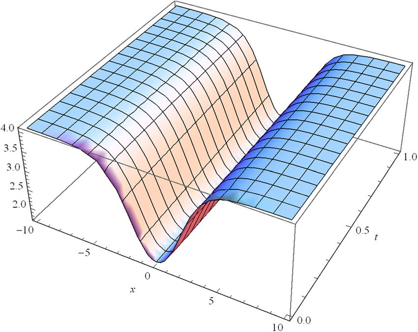
114 Hadi Rezazadeh et al.
From (14), we deduce the following exact solutions:
−2(α2γ + β)
q1(x , t ) = ± tanh(x − νt )
4β 2 ω 2 + 4αβω + α2 + 8βγ
1 1 2
× exp i − 1 ± 8 −γω 2β + γωα + 2γ 2 − βω + α
1
2γ 4 2
2
1
1 2
× β ω + β(αω + 2γ ) + α (4β ω + 4αβω + α + 8βγ ) x + ωt + θ0 ,
2 2 2 2 2 −1
4
and
−2(α2γ + β)
q2(x , t ) = ± coth(x − νt )
4β 2 ω 2 + 4αβω + α2 + 8βγ
1 1 2
× exp i − 1 ± 8 −γω 2β + γωα + 2γ 2 − βω + α
1
2γ 4 2
2
1
1 2
× β ω + β(αω + 2γ ) + α (4β ω + 4αβω + α + 8βγ ) x + ωt + θ0 .
2 2 2 2 2 −1
4
Case II:
−2(α2γ + β)
A0 = 0, A1 = 0, B1 = ± , B1 = 0,
−4β 2 ω 2 − 4αβω − α2 + 4βγ
) .
2
κ=
1
1 8
( 1
)(
1
)( 1
− γω 2β + γωα − γ 2 − 4 βω + 2 α β 2 ω 2 + β(αω − γ ) + 4 α2
2γ
±
−4β 2 ω 2 − 4αβω − α2 + 4βγ
From (14), we deduce the following exact solutions:
−2(α2γ + β)
q3(x , t ) = ± sech(x − νt )
−4β 2 ω 2 − 4αβω − α2 + 4βγ
1 1 2
× exp i − 1 ± 8 −γω 2β + γωα − γ 2 − βω + α
1
2γ 4 2
2
1
× β 2 ω 2 + β(αω − γ ) + α2 (−4β 2 ω 2 − 4αβω − α2 + 4βγ )−1 x + ωt + θ0 ,
1
4
and
2(α2γ + β)
q4(x , t ) = ± csch(x − νt )
−4β 2 ω 2 − 4αβω − α2 + 4βγ
1 1 2
× exp i − 1 ± 8 −γω 2β + γωα − γ 2 − βω + α
1
2γ 4 2
2
1
× β 2 ω 2 + β(αω − γ ) + α2 (−4β 2 ω 2 − 4αβω − α2 + 4βγ )−1 x + ωt + θ0 .
1
4
On the optical solutions to NLSE with second-order spatiotemporal dispersion 115
Case III:
1 −2(α2γ + β) 1 2(α2γ + β)
A0 = 0, A1 = ± , B1 = ± ,
2 4β 2 ω 2 + 4αβω + α2 + 2βγ 2 4β 2 ω 2 + 4αβω + α2 + 2βγ
1 −(4γω 2β + 4γωα + 2γ 2 − 1)(2βω + α)2 (4β 2 ω 2 + 2β(2αω + γ ) + α2)
κ= 1 ± .
2γ 4β 2 ω 2 + 4αβω + α2 + 2βγ
From (14), we deduce the following exact solutions:
2(α2γ + β)
q5(x , t ) = ± (sech(x − νt ) + i tanh(x − νt ))
4β 2 ω 2 + 4αβω + α2 + 2βγ
1
× exp i − (1 ± ((−(4γω 2β + 4γωα + 2γ 2 − 1)(2βω + α)2
2γ
× (4β 2 ω 2 + 2β(2αω + γ ) + α2))(4β 2 ω 2 + 4αβω + α2 + 2βγ )−1 )2 x + ωt + θ0 ,
) )
1
and
−2(α2γ + β)
q6(x , t ) = ± (csch(x − νt ) + coth(x − νt ))
4β 2 ω 2 + 4αβω + α2 + 2βγ
1
× exp i − (1 ± ((−(4γω 2β + 4γωα + 2γ 2 − 1)(2βω + α)2
2γ
× (4β 2 ω 2 + 2β(2αω + γ ) + α2))(4β 2 ω 2 + 4αβω + α2 + 2βγ )−1 )2 x + ωt + θ0 .
) )
1
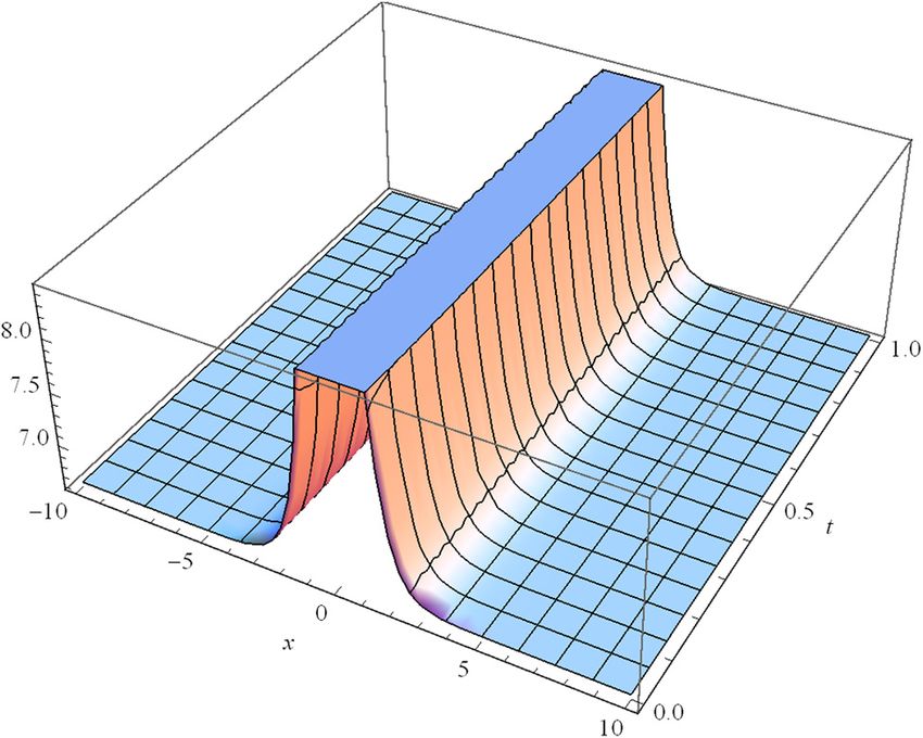
Figure 1: Graphical representation of solution q1(x , t ) with the Figure 2: Graphical representation of solution q3(x , t ) with the
parameter values as: ς1 = 2, ς2 = 3, ς3 = 1, ϑ1 = 3, ϑ2 = 1 , ϑ3 = 1 , parameter values as: ς1 = 2, ς2 = 3, ς3 = 1, ϑ1 = 5, ϑ2 = 3, ϑ3 = 2,
α = 3, β = 2 , γ = 4 , μ = 3, ν = 2, ω = 3 . α = −1 , β = 2, γ = −2, μ = 2, ν = −2, ω = 3.
4 Graphical representation of 5 Conclusions
solutions In this study, the sine-Gordon expansion method was
In this section, the solitons solution for the main equation employed to integrate the NLSE with the coefficients of
for different cases and different values of the parameters group velocity dispersion and second-order spatiotem-
is being investigated and represented throughout the poral dispersion. Some new traveling wave solutions
following figures with the help of Mathematica 11.0. are found while changing the values of the parameters.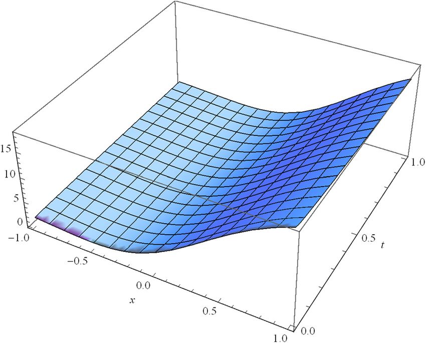
116 Hadi Rezazadeh et al.
Figure 3: Graphical representation of solution q3(x , t ) with the Figure 5: Graphical representation of solution q5(x , t ) with the
parameter values as: ς1 = 2, ς2 = 4, ς3 = 1 , ϑ1 = 1, ϑ2 = 2, ϑ3 = 3, parameter values as: ς1 = 2, ς2 = −3, ς3 = 4, ϑ1 = 0, ϑ2 = −1 , ϑ3 = 1 ,
α = 3, β = 2, γ = −2, μ = 2, ν = 3, ω = 2. α = −4, β = 2, γ = −2, μ = 2, ν = 1 , ω = −3, λ1 = −1 , λ2 = 1 .
Figure 4: Graphical representation of solution q4(x , t ) with the Figure 6: Graphical representation of solution q6(x , t ) with the
parameter values as: ς1 = 2, ς2 = 3, ς3 = 5, ϑ1 = 4, ϑ2 = 5, ϑ3 = 3, parameter values as: ς1 = 2, ς2 = 1 , ς3 = 3, ϑ1 = 0, ϑ2 = 3, ϑ3 = −2,
α = 4, β = 3, γ = −4, μ = 2, ν = 2, ω = 3. α = 4 , β = 2 , γ = 2, μ = 2 , ν = 4 , ω = 2 .
The new form of solutions possesses some novel traveling Acknowledgements: The authors would like to express
wave behaviors. A graphical representation of these solu- their sincere thanks to the support of National Natural
tions is provided in Figures 1–6. The proposed method is Science Foundation of China.
shown to provide a solution with important physical
representation which may help in dealing with similar
Conflict of interest: Authors state no conflict of interest.
complex nonlinear models with applications in contem-
porary science and other related areas. The method proves
to be a reliable method for solving such models with high Funding information: This work was supported by the
accuracy. This work, thus, provides a lot of encouragement National Natural Science Foundation of China (Grant
for subsequent research in this area, and the results of that Nos. 11971142, 11871202, 61673169, 11701176, 11626101, and
research will be reported in near future. 11601485).On the optical solutions to NLSE with second-order spatiotemporal dispersion 117
Author contributions: All authors have accepted respon- [15] Khater MM, Lu D, Hamed YS. Computational simulation for the
sibility for the entire content of this manuscript and (1+1)-dimensional Ito equation arising quantum mechanics
approved its submission. and nonlinear optics. Results Phys. 2020 Dec 1;19:103572.
[16] Abdel-Aty AH, Khater MM, Baleanu D, Khalil EM, Bouslimi J,
Omri M. Abundant distinct types of solutions for the nervous
biological fractional FitzHugh-Nagumo equation via three
different sorts of schemes. Adv Differ Equ. 2020
Dec;2020(1):1–7.
References [17] Chu Y, Khater MM, Hamed YS. Diverse novel analytical and
semi-analytical wave solutions of the generalized (2+1)-
[1] Jajarmi A, Ghanbari B, Baleanu D. A new and efficient numer- dimensional shallow water waves model. AIP Advances. 2021
ical method for the fractional modeling and optimal control of Jan 1;11(1):015223.
diabetes and tuberculosis co-existence. Chaos: [18] Srivastava HM, Baleanu D, Machado JA, Osman MS,
Interdisciplinary J Nonlin Sci. 2019 Sep 9;29(9):093111. Rezazadeh H, Arshed S, Günerhan H. Traveling wave solutions
[2] Qureshi S, Yusuf A, Shaikh AA, Inc M, Baleanu D. Fractional to nonlinear directional couplers by modified Kudryashov
modeling of blood ethanol concentration system with real data method. Physica Scripta. 2020 Jun 1;95(7):075217.
application. Chaos: Interdisciplinary J Nonlin Sci. 2019 Jan [19] Ghanbari B, Nisar KS, Aldhaifallah M. Abundant solitary wave
31;29(1):013143. solutions to an extended nonlinear Schrödinger’s equation
[3] Jajarmi A, Arshad S, Baleanu D. A new fractional modelling and with conformable derivative using an efficient integration
control strategy for the outbreak of dengue fever. Physica A: method. Adv Differ Equ. 2020 Dec;2020(1):1–25.
Stat Mech Appl. 2019 Dec 1;535:122524. [20] Ghanbari B, Yusuf A, Baleanu D. The new exact solitary wave
[4] Qureshi S, Rangaig NA, Baleanu D. New numerical aspects of solutions and stability analysis for the (2+1)-dimensional
Caputo-Fabrizio fractional derivative operator. Mathematics. Zakharov-Kuznetsov equation. Adv Differ Equ. 2019
2019 Apr;7(4):374. Dec;2019(1):1–5.
[5] Munawar M, Jhangeer A, Pervaiz A, Ibraheem F. New general [21] Munusamy K, Ravichandran C, Nisar KS, Ghanbari B. Existence
extended direct algebraic approach for optical solitons of of solutions for some functional integrodifferential equations
Biswas-Arshed equation through birefringent fibers. Optik. with nonlocal conditions. Math Meth Appl Sci. 2020 Nov
2021 Feb 1;228:165790. 30;43(17):10319–31.
[6] Jhangeer A, Hussain A, Junaid-U-Rehman M, Baleanu D, [22] Inc M, Khan MN, Ahmad I, Yao SW, Ahmad H, Thounthong P.
Riaz MB. Quasi-periodic, chaotic and travelling wave struc- Analysing time-fractional exotic options via efficient local
tures of modified Gardner equation. Chaos, Solitons & meshless method. Results Phys. 2020 Dec 1;19:103385.
Fractals. 2021 Feb 1;143:110578. [23] Rezazadeh H, Inc M, Baleanu D. New solitary wave solutions
[7] Hussain A, Jhangeer A, Abbas N, Khan I, Sherif ES. Optical for variants of (3+1)-dimensional
solitons of fractional complex Ginzburg–Landau equation with Wazwaz–Benjamin–Bona–Mahony equations. Front Phys.
conformable, beta, and M-truncated derivatives: a compara- 2020 Sep 4;8:332.
tive study. Adv Differ Equ. 2020 Dec;2020(1):1–9. [24] Khater MM, Inc M, Attia RA, Lu D, Almohsen B. Abundant new
[8] Hosseini K, Osman MS, Mirzazadeh M, Rabiei F. Investigation computational wave solutions of the GM-DP-CH equation via
of different wave structures to the generalized third-order two modified recent computational schemes. J Taibah Univ Sci.
nonlinear Scrödinger equation. Optik. 2020 Mar 2020 Jan 1;14(1):1554–62.
1;206:164259. [25] Rahman G, Nisar KS, Ghanbari B, Abdeljawad T. On general-
[9] Hosseini K, Mirzazadeh M, Vahidi J, Asghari R. Optical wave ized fractional integral inequalities for the monotone weighted
structures to the Fokas-Lenells equation. Optik. 2020 Apr Chebyshev functionals. Adv Differ Equ. 2020 Dec;2020(1):1–9.
1;207:164450. [26] Akinyemi L, Senol M, Huseen SN. Modified homotopy methods
[10] Rezazadeh H. New solitons solutions of the complex for generalized fractional perturbed Zakharov–Kuznetsov
Ginzburg–Landau equation with Kerr law nonlinearity. Optik. equation in dusty plasma. Adv Differ Equ. 2021
2018 Aug 1;167:218–27. Dec;2021(1):1–27.
[11] Hosseini K, Mirzazadeh M, Ilie M, Gómez-Aguilar JF. Biswas- [27] Akinyemi L. A fractional analysis of Noyes-Field model for the
Arshed equation with the beta time derivative: optical solitons nonlinear Belousov–Zhabotinsky reaction. Comput Appl Math.
and other solutions. Optik. 2020 Sep 1;217:164801. 2020 Sep;39:1–34.
[12] Yokus A, Durur H, Ahmad H, Thounthong P, Zhang YF. [28] Akinyemi L, Senol M, Iyiola OS. Exact solutions of the
Construction of exact traveling wave solutions of the generalized multidimensional mathematical physics
Bogoyavlenskii equation by (G ∕ G, 1 ∕ G)-expansion and (1 ∕ G)- models via sub-equation method. Math Comput Simul. 2021
expansion techniques. Results Phys. 2020 Dec 1;19:103409. April 1;182:211–33.
[13] Yokus A, Durur H, Ahmad H. Hyperbolic type solutions for the [29] Senol M, Iyiola OS, Kasmaei HD, Akinyemi L. Efficient analy-
couple Boiti-Leon-Pempinelli system. Facta Universitatis, tical techniques for solving time-fractional nonlinear coupled
Series: Mathematics and Informatics. 2020 May Jaulent-Miodek system with energy-dependent Schrödinger
28;35(2):523–31. potential. Adv Differ Equ. 2019 Dec;2019(1):1–21.
[14] Yokus A, Durur H, Ahmad H, Yao SW. Construction of different [30] Khater MM. On the dynamics of strong Langmuir turbulence
types analytic solutions for the Zhiber-Shabat equation. Math. through the five recent numerical schemes in the plasma
2020 Jun;8(6):908. physics. Numer Methods Partial Differ Equ. 2020 Dec 4.118 Hadi Rezazadeh et al.
[31] Tariq KU, Seadawy AR. On the soliton solutions to the modified arising in fluid dynamics. Nonlin Dyn. 2016 Oct;
Benjamin-Bona-Mahony and coupled Drinfelad-Sokolov- 86(1):177–83.
Wilson models and its applications. J King Saud Univ Sci. 2020 [44] Yel G, Baskonus HM, Bulut H. Novel archetypes of new coupled
Jan 1;32(1):156–62. Konno-Oono equation by using sine-Gordon expansion
[32] Bhrawy AH, Biswas A, Javidi M, Ma WX, Pınar Z, Yıldırım A. New method. Opt Quant Electron. 2017 Sep;49(9):1–10.
solutions for (1+1)-dimensional and (2+1)-dimensional Kaup- [45] Yel G, Baskonus HM, Gao W. New dark-bright soliton in the
Kupershmidt equations. Results Math. 2013 shallow water wave model. Aims Math. 2020 Apr
Feb;63(1):675–86. 20;5(4):4027–44.
[33] Mirzazadeh M, Eslami M, Zerrad E, Mahmood MF, Biswas A, [46] Ismael HF, Bulut H, Baskonus HM. Optical soliton solutions to the
Belic M. Optical solitons in nonlinear directional couplers by Fokas-Lenells equation via sine-Gordon expansion method and
sine-cosine function method and Bernoulli’s equation (m + (G ′∕G))-expansion method. Pramana. 2020 Dec;94(1):1–9.
approach. Nonlin Dyn. 2015 Sep;81(4):1933–49. [47] Ali KK, Wazwaz AM, Osman MS. Optical soliton solutions to the
[34] Qiao Z. Darboux transformation and explicit solutions for two generalized nonautonomous nonlinear Schrödinger equations
integrable equations. J Math Anal Appl. 2011 Aug in optical fibers via the sine-Gordon expansion method. Optik.
15;380(2):794–806. 2020 Apr 1;208:164132.
[35] Wazwaz AM, El-Tantawy SA. Solving the (3+1)-dimensional KP- [48] Korkmaz A, Hepson OE, Hosseini K, Rezazadeh H, Eslami M.
Boussinesq and BKP-Boussinesq equations by the simplified Sine-Gordon expansion method for exact solutions to con-
Hirota’s method. Nonlin Dyn. 2017 Jun;88(4):3017–21. formable time fractional equations in RLW-class. J King Saud
[36] Yang S, Hua C. Lie symmetry reductions and exact solutions of Univ Sci. 2020 Jan 1;32(1):567–74.
a coupled KdV-Burgers equation. Appl Math Comput. 2014 [49] Leta TD, El Achab A, Liu W, Ding J. Application of bifurcation
May 15;234:579–83. method and rational sine-Gordon expansion method for sol-
[37] Younis M. A new approach for the exact solutions of nonlinear ving 2D complex Ginzburg–Landau equation. Int J Mod Phys B.
equations of fractional order via modified simple equation 2020 Apr 10;34(9):2050079.
method. Appl Math. 2014 Jul 7;5(13):1927–32. [50] Tasbozan O, Kurt A. The new travelling wave solutions of time
[38] Ablowitz MJ, Ablowitz MA, Clarkson PA, Clarkson PA. Solitons, fractional Fitzhugh–Nagumo equation with Sine-Gordon
nonlinear evolution equations and inverse scattering. London: expansion method. Adıyaman Universitesi Fen Bilimleri
Cambridge University Press; 1991 Dec 12. Dergisi. 2020 June 26;10(1):256–63.
[39] Hirota R. Exact solution of the Korteweg-de Vries equation for [51] Tariq KU, Younis M. Bright, dark and other optical solitons with
multiple collisions of solitons. Phys Rev Lett. 1971 Nov second order spatiotemporal dispersion. Optik. 2017 Aug
1;27(18):1192. 1;142:446–50.
[40] Wang M. Exact solutions for a compound KdV-Burgers equa- [52] Christian JM, McDonald GS, Hodgkinson TF, Chamorro-
tion. Phys Lett A. 1996 Apr 29;213(5–6):279–87. Posada P. Wave envelopes with second-order spatiotemporal
[41] Tariq KU, Seadawy AR, Younis M, Rizvi ST. Dispersive traveling dispersion. I. Bright Kerr solitons and cnoidal waves. Phys Rev
wave solutions to the space-time fractional equal-width A. 2012 Aug 21;86(2):023838.
dynamical equation and its applications. Opt Quant Electron. [53] Christian JM, McDonald GS, Hodgkinson TF, Chamorro-
2018 Mar;50(3):1–6. Posada P. Wave envelopes with second-order spatiotemporal
[42] Tariq KU, Seadawy AR. Bistable Bright-Dark solitary wave dispersion. II. Modulational instabilities and dark Kerr soli-
solutions of the (3+1)-dimensional Breaking soliton, tons. Phys Rev A. 2012 Aug 21;86(2):023839.
Boussinesq equation with dual dispersion and modified [54] Rezazadeh H, Mirhosseini-Alizamini SM, Neirameh A,
Korteweg-de Vries-Kadomtsev-Petviashvili equations and Souleymanou A, Korkmaz A, Bekir A. Fractional Sine-Gordon
their applications. Results Phys. 2017 Jan 1;7:1143–9. equation approach to the coupled Higgs system defined in
[43] Baskonus HM. New acoustic wave behaviors to the time-fractional form. Iran J Sci Technol Trans A: Sci. 2019
Davey-Stewartson equation with power-law nonlinearity Dec;43(6):2965–73.You can also read