Optimal Allocations to Heterogeneous Agents with an Application to the COVID-19 Stimulus Checks - Vegard M. Nygaard, Bent E. Sorensen, Fan Wang ...
←
→
Page content transcription
If your browser does not render page correctly, please read the page content below
Optimal Allocations to Heterogeneous Agents
         with an Application to the
        COVID-19 Stimulus Checks

   Vegard M. Nygaard, Bent E. Sorensen, Fan Wang

                  Department of Economics
                   University of Houston

                      June 25, 2021

        paper pdf | project website | abstract | slides

                                                          1/21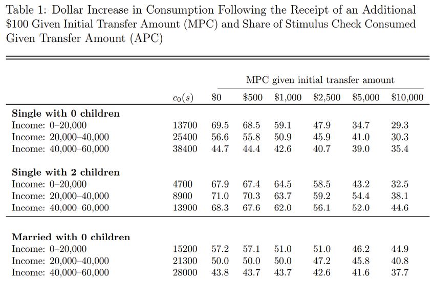
Motivation: Allocation Among Heterogeneous Agents

 1. Nutrition
      • Height/stunting in the absence of supplements (Ai )
      • Marginal effects of protein or rice supplements (αi )
 2. Job training
      • Employment probability without training (Ai )
      • Marginal effects of training (αi )
 3. Heterogeneity by demographic and human-capital attributes
 4. Given observables, what are the allocative implications of
    estimates and predictions from reduced-form or structural
    models?

                                                                 2/21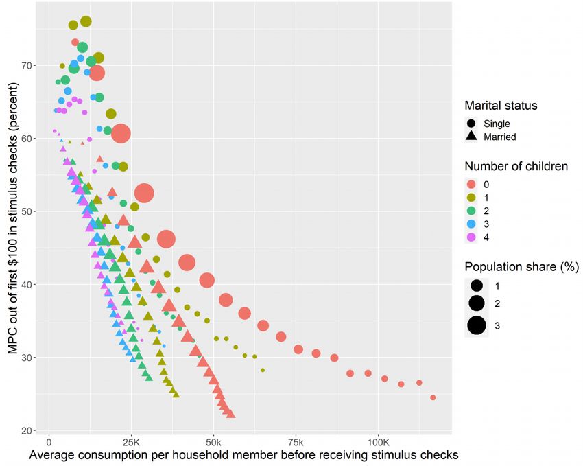
Motivation: COVID-19 Stimulus Checks

1. Trump checks (CARES Act)
     • $1200 per spouse, $500 per child
     • Married phase-out starts at $150,000, decrease by $5 for
       every additional $100 in income
2. Biden checks (ARRA Act)
     • $1400 per spouse, $1400 per child
     • Married phase-out starts at $150,000, zero after $160,000
3. Focus on consumption response, goal of policy
     • Consumption without stimulus (Ai )
     • Consumption gain from one more $100 check (αi )
4. How to gauge welfare among alternatives? What is optimal?

                                                                   3/21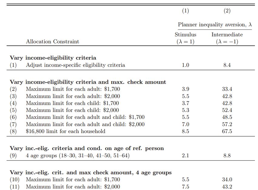
Literature

1. No prior work studying the optimal allocation of COVID-19
   stimulus checks (Falcettoni and Nygaard 2021)
2. Optimal policy literature often rely on first order conditions to
   design parametric policy-rules that are optimal for an
   Utilitarian planner. We have:
     • Analytical solutions without FOC
     • Individually-constrained optimal allocations
     • Heterogeneous planner preferences

                                                                       4/21
The Allocation Problem

A planner affects changes in some individual outcome Hi
(consumption in 2021) with individual specific allocation Vi
(stimulus check amounts), whose effects depend on observables x i
(marital stuats, number of children, income) and estimates θ i
(structural parameters):

                            H (Vi ; x i , θ i )

Planners aggregate Hi , and differ in inequality aversion and biases.

                                                                        5/21
The Allocation Problem
Given Atkinson preferences (CES aggregation) (Atkinson 1970):
!1
N λ
U {Hi }N
i=1 = ∑ βi (H (Vi ; x i , θ i ))λ ,
i=1
(1)
N
where βi > 0 , ∑ βi = 1, and − ∞ < λ ≤ 1 ,
i=1
on the constraint choice set
N
C ≡ V = (V1 , · · · , VN ) : 0 ≤ Vi ∈ Ωi , and, c ∈ R+
∑ Vi ≤ W .
i=1
(2)
6/21The Allocation Problem: Breaking Standard CES
Under the standard CES problem, Hi is proportional in Vi :
!1
N λ
max
{Vi }N
∑ βi (Hi )λ (3)
i=1 i=1
s.t. ∀ i, Hi = αi Vi and 0 ≤ Vi , and ΣN
i=1 Vi = W
c
Three CES allocative assumptions (aspects of Inada) that the
stimulus checks problem breaks:
1. Hi (Vi = 0) = 0, but empirically, Hi (Vi = 0) > 0 possible
2. The objective function is continuously differentiable in Vi
3. No potential binding constraints on Vi
7/21Discrete Choice Set
Discrete problems: bags of rice, pre-natal check-up slots, training
spots, or stimulus checks. The discrete choice set is:
(
n o
C ≡ D = (D1 , · · · , DN ) : Di ∈ D i , D i + 1, · · · , D̄i ,
D
¯ ¯
) (4)
N
D i ∈ N0 , ∑ Di ≤ W c .
¯ i=1
• Nests continuous choices
• Upper and lower bounds on allocations Di
• Binary if D i = D = 0 and D̄i = D̄ = 1
¯ ¯
Wc+N−1) !
• Number of choices between N! and
N−W !W !
c c (N−1))!W
c!
8/21Discrete Input Output
Without imposing structural or parametric assumptions, for
individual i, l indexes each increment of discrete allocations:
D̄i
Hi = Ai + ∑ αil · 1 l ≤ Di . (5)
l=1
1. Consumption without checks: Ai
2. MPC: αil is the i and increment specific effects
9/21Discrete Assumption
Assumption
Marginal effects αil for the l th increment of Di on Hi are: (1)
positive, αil > 0; (2) non-increasing, αil ≤ αi,l−1 ; and (3) can lead
i −1
to positive outcomes, Ai + ∑D̄ l=1 αil > 0.
1. The first restriction is innocuous
2. The second restriction accommodates both constant returns,
as well as arbitrarily step functions of decreasing returns
3. The third restriction allows for Ai > 0 or Ai < 0
10/21Discrete Problem
Definition
Optimal
allocation functions D∗ = (D1∗ , · · · , DN∗ ),
n oN
∗ N N D̄i N
Dj W , λ , {βi }i=1 , {Ai }i=1 , {αil }l=1
c , D i , D̄i i=1 : N ×
i=1 ¯
N
N N (∑i=1 D̄i ) (N·2)
(−∞, 1] × (0, 1) × R × R+ × N0 → D j , D j + 1, · · · , D̄j
, maximize ¯ ¯
! 1
N D̄i
λ λ
(6)
max ∑ βi Ai + ∑ αil · 1 l ≤ Di ,
D∈C D i=1 l=1
N
on the constraint set C D W
c, D , D̄i
i i=1
.
¯
11/21Discrete Theorem Intuition
Solve for a resource-invariant optimal allocation queue QilD :
• The queue is ranked from 1 to ∑N i=1 D̄i .
D
• Qil = 1 is the top ranked individual.
• If an individual has two units of allocations ranked at the 1st
and the 4th spot of the queue, when aggregate resources is
equal to 4, the individual receives both units of allocation.
Under Assumption 1, as W c increases, the planner will only allocate
more to individuals—the discrete resource (income) expansion path
does not bend backwards.
12/21Discrete Theorem
Theorem
Given Assumption 1 and assume WLOG D i = 0, then:
¯
D̄i n o
Di∗ = ∑ 1 QilD ≤ W
c (7)
l=1
!λ !λ
l
e l−1
e
−
D̄
Aei + ∑ αeil 0 Ai
+ ∑ α il 0
N i
0
e
0
e
l =1 l =0
e β
D i
Qil = ∑ ∑ 1 · ≥ 1 .
e
λ λ
βi l l−1
i=1 l=1
− Ai + ∑ αil 0
Ai + ∑ αil 0
e e
l 0 =1 l 0 =0
(8)
13/21Life-cycle Consumption and Savings Model
We develop a dynamic life-cycle model:
1. Ex-ante heterogeneity in discount factor, education and
marital status
2. Household-head and spousal stochastic income process and
child (up to 4) transition process
3. Endogenous consumption and savings choices
4. Equilibrium in government spending and revenue
COVID-19:
1. Unexpected unemployment shock with partial UI benefits in
2020 and 2021 (MIT shocks)
2. Possibly lock-down effects on consumption
3. Optimal policy in for 2021 given 2020 information
14/21Model Predictions: Ai and αi,1
15/21Model Predictions: αil
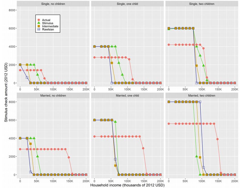
16/21Optimal Policy Three Planners
17/21Perturbing Ai and Bounds
18/21The Allocation Queue
19/21Tradeoffs Between Policies
20/21Conclusion and Summary
We developed an optimal allocation framework:
1. Heterogenous preferences
2. Arbitrary individual bounds
3. Derivative-free (non-increasing)
4. Linearly increasing computational cost with N
COVID-19 Stimulus Checks:
1. Negatively correlated Ai and αi
2. Allocate more to poorer
3. Framework to evaluate trade-offs across allocation rules.
21/21You can also read