Genome assembly with ALLPATHS- LG: How to make it work
←
→
Page content transcription
If your browser does not render page correctly, please read the page content below
Genome
assembly
with
ALLPATHS-‐LG:
How
to
make
it
work
How to use ALLPATHS-‐LG What you will need: -‐ High-‐quality data -‐ Libraries of different sizes -‐ Long mate-‐pair links (40kb): difficult to make libraries!! -‐ A BIG compute server: recommended at least 1TB of RAM
Preparing data for ALLPATHS-‐LG Before assembling, prepare and import your read data. ALLPATHS-‐LG expects reads from: • At least one fragment library. One should come from fragments of size ~180 bp. This isn’t checked but otherwise results will be bad. • At least one jumping library. IMPORTANT: use all the reads, including those that fail the Illumina purity filter (PF). These low quality reads may cover ‘difficult’ parts of the genome.
ALLPATHS-‐LG
input
format
ALLPATHS-‐LG
can
import
data
from:
BAM,
FASTQ,
FASTA/QUALA
or
FASTB/QUALB
files.
You
must
also
provide
two
metadata
files
to
describe
them:
in_libs.csv
-‐
describes
the
libraries
in_groups.csv
-‐
_es
files
to
libraries
FASTQ
format:
consists
of
records
of
the
form
@
+
Libraries – in_libs.csv (1 of 3) in_libs.csv is a comma separated value (CSV) file. For clarity, blanks and tabs are allowed and ignored. The first line describes the field names, listed below. Each subsequent line describes a library. library_name -‐ a unique name for the library. Each physically different library should have a different name!
Libraries – in_libs.csv (2 of 3) For fragment libraries only frag_size -‐ es_mated mean fragment size frag_stddev -‐ es_mated fragment size std dev For jumping libraries only insert_size -‐ es_mated jumping mean insert size insert_stddev -‐ es_mated jumping insert size std dev These values determine how a library is used. If insert_size is ≥ 20000, the library is assumed to be a Fosmid jumping library. paired -‐ always 1 (only supports paired reads) read_orientation -‐ inward or outward. Paired reads can either point towards each other, or away from each other. Currently fragment reads must be inward, jumping reads outward, and Fosmid jumping reads inward.
Libraries
–
in_libs.csv
(3
of
3)
Reads
can
be
trimmed
to
remove
non-‐genomic
bases
produced
by
the
library
construc_on
method:
genomic_start
genomic_end - inclusive zero-based range of read bases
to be kept; if blank or 0 keep all bases
Reads
are
trimmed
in
their
original
orienta_on.
Extra
op_onal
fields
(descrip_ve
only
–
ignored
by
ALLPATHS)
project_name
-‐
a
string
naming
the
project.
organism_name
-‐
the
organism
name.
type
-‐
fragment,
jumping,
EcoP15I,
etc.
EXAMPLE
library_name, type, paired, frag_size, frag_stddev, insert_size, insert_stddev, read_orientation, genomic_start, genomic_end
Solexa-11541, fragment, 1, 180, 10, , , inward ,
Solexa-11623, jumping, 1, , , 3000, 500, outward 0, 25Input
files
–
required
format
Each
BAM
or
FASTQ
file
contains
paired
reads
from
one
library.
Data
from
a
single
library
can
be
split
between
files.
Example,
one
file
for
each
Illumina
lane
sequenced.
For
FASTQ
format,
the
paired
reads
can
be
divided
in
two
files
(readsA.fastq,
readsB.fastq),
or,
if
in
a
single
file
(reads.fastq),
must
be
interleaved:
pair1_readA
pair1_readB
pair2_readA
pair2_readB
…Input
files
–
in_groups.csv
Each
line
in
in_groups.csv
comma
separated
value
file,
corresponds
to
a
BAM
or
FASTQ
file
you
wish
to
import
for
assembly.
The
library
name
must
match
the
names
in
in_libs.csv.
group_name
-‐
a
unique
nickname
for
this
file
library_name
-‐
library
to
which
the
file
belongs
file_name
-‐
the
absolute
path
to
the
file
(should
end
in
.bam
or
.fastq)
(use
wildcards
‘?’,
‘*’
for
paired
fastqs)
Example:
group_name, library_name, file_name
302GJ, Solexa-11541, /seq/Solexa-11541/302GJABXX.bam
303GJ, Solexa-11623, /seq/Solexa-11623/303GJABXX.?.fastqALLPATHS-‐LG
directory
structure
PrepareAllPathsInputs.pl
You
create.
You
create.
Root
for
your
Generally
one
assemblies.
per
data
set.
Fixed
name.
////ASSEMBLIES/test
You
create.
You
provide
Fixed
name.
Where
Generally
one
name.
One
per
you’ll
find
per
organism.
assembly.
assembly
results.
RunAllPaths3G
How
  to
  import
  assembly
  data
  files


PrepareAllPathsInputs.pl
    IN_GROUPS_CSV=
    IN_LIBS_CSV=
    DATA_DIR=
    PLOIDY=
    PICARD_TOOLS_DIR=
    HOSTS=

• IN_GROUPS_CSV and IN_LIBS_CSV: optional arguments with default
values ./in_groups.csv and ./in_libs.csv. These arguments
determine where the data are found.

• DATA_DIR:
  imported
  data
  will
  be
  placed
  here.


(con'nued)
How to assemble Do this: RunAllPathsLG \ PRE= \ REFERENCE_NAME= \ DATA_SUBDIR= \ RUN= Automa_c resump_on. If the pipeline crashes, fix the problem, then run the same RunAllPathsLG command again. Execu_on will resume where it leq off. Results. The assembly files are: final.contigs.fasta -‐ fasta con_gs final.contigs.efasta -‐ efasta con_gs final.assembly.fasta -‐ scaffolded fasta final.assembly.efasta -‐ scaffolded efasta
Linearized
  graph
  assemblies


Example of an assembly in efasta format
>scaffold_1!
TCCTAGATCCACTTGGACTTGAGCTTTGTATATATATATATATATATA{,TA}CAAGATGACATATATAGGAGACAGCCA!
GTTATACCAGCACCATTTATTGAAGACACTTTCTTTATTCCATTGTATATTTTTTTACTTCCTTGTCAAAAATCAAGTGA!
CCATGAGTATGTGGTTTCATTTCTGGGTCTTCAATTGTATTCCATTAGTCAACATATCTGTCTCTGTACCAATACCATGC!
NNNNNNNN!
AGTTTTTACCACAATTGCTCTATAGTAAAGCTTGAGGTCAGGGTTGGTGATCCCTCCAGCCATTCTTTCATTATTAAGAA!
TTGTTTTCCCTAGTCTGGGTTTTTTGCTTTTCCAGGCGAATTTGAGAATTGCTCTTTCCATGTCTTTGAAGAATTGTGTT!
NNNNNNNNNNNNNNNNNNNNNNNNNNNNNNNNNNNN!
GGGATTTTGATGGGGTTTGCATTGAATCTGTAGATTGTCTTTGGTAAGATGGTTAGTTTTACTATGTTAATTCTGCCAAT!
CCACAAGCATGGGAGCGCTCTCCATTTTCTGAGATCTTCTTCAATTTCTTTCTTGAGAAACTTGAAGTTATTGTCATACA!
>scaffold_2!
CTGAAGTTGTTTATCAGCTGGAGAAGTTCTCAGGTAGAATTTTTGGGATT{A,C,G}GCTTATGTATGCTATCTTGCAAA!
TAGTGATACCTTGATTTCTTTTTTACCAATATGTATCCCATTGATCTCTTTCTGTTGTCTTATTGTTCTAGCTAACACTT!
CAAGTACTATATTGAATAGATATGGGGAGAGTGGGAATCCTTGTCTTGTCTCCGATTTCAGTGGGATTGCTTCAAGTATG!
Metrics, output and diagnosQcs final.assembly.efasta ! final.contigs.efasta ! final.contigs.fastb ! final.summary ! final.assembly.fasta ! final.contigs.fasta ! final.rings ! final.superb ! assembly_stats.report! library_coverage.report! Metric: N50 “length-‐weighted median” ⇒ 50% of sequences are this long or longer
Things
  that
  can
  go
  wrong


•
  Not
  enough
  RAM

•
  Not
  enough
  CPU
  _me
  (allpaths
  can
  resume
  from
  where
  it
  died!)


•
  Ar_facts
  in
  the
  data
ComputaQonal
requirements
•
64-‐bit
Linux
•
runs
mul_-‐threaded
on
a
single
machine
•
memory
requirements
o
about
160
bytes
per
genome
base,
implying
need
512
GB
for
mammal
(Dell
R315,
48
processors,
€18,000)
need
1
GB
for
bacterium
(theore_cally)
o
if
coverage
different
than
recommended,
adjust!
o
poten_al
for
reducing
usage
•
wall
clock
_me
to
complete
run
o
5
Mb
genome
1
hour
(8
processors)
o
2500
Mb
genome
500
hours
(48
processors)
Short
jumping
libraries
(2-‐3
kb)
10
μg
DNA
Illumina
protocol,
blunt-‐
shear
and
size
select
end
liga_on
2-‐3
kb
fragments
bio_nylate
ends
shear
and
select
Short jumping libraries (2-‐3 kb) Problem 1. Many steps many opportuni_es for failure. Example: a reagent might degrade. (This has happened.)
Short jumping libraries (2-‐3 kb) Problem 2. Many steps many DNA losses. Here are good results for a mammalian genome: Input: 10 μg DNA ~3,000,000x physical coverage Output: (if fully sequenced) ~3,000x physical coverage Loss: 99.9% (not including DNA between reads) Small genomes are much easier!
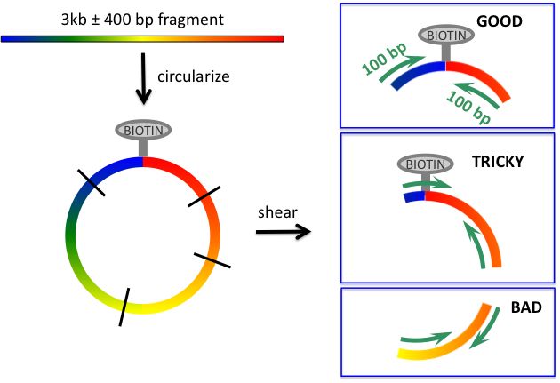
Short jumping libraries (2-‐3 kb) Problem 3. Read passes through circulariza_on junc_on. This reduces the effec_ve read length (and complicates algorithm). What might be done to reduce incidence of this: shear circles to larger size and select larger fragments
Short jumping libraries (2-‐3 kb) Problem 4. Reads come from nonjumped fragments and are thus in reverse orienta_on and close together on the genome. This reduces yield (and complicates algorithm). Puta_ve cause: original DNA is nicked or becomes nicked during process – bio_ns become ‘ectopically’ ayached at these nicks
Long jumping libraries (~6 kb) Method 1. Instead of shearing circles, using EcoP15I restric_on enzyme. Pros -‐ demonstrated to work -‐ no ar_facts Cons -‐ read length = 26 bases Method 2. Use Illumina blunt-‐end liga_on protocol, but shear and size select larger fragments. Pros -‐ long reads Cons -‐ yield may be very low (probably not problem for small genomes)
You can also read