Organismal Biology A Journal of the Society for Integrative and Comparative Biology
←
→
Page content transcription
If your browser does not render page correctly, please read the page content below
Downloaded from https://academic.oup.com/iob/article/2/1/obaa009/5818881 by guest on 15 October 2020
 Integrative
Organismal
       Biology   A Journal of the Society
                 for Integrative and
                 Comparative Biology

                 academic.oup.com/icb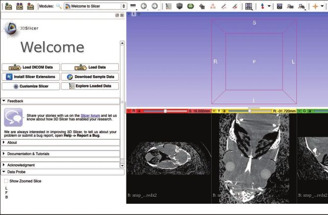
Integrative Organismal Biology
Integrative Organismal Biology, pp. 1±25
doi:10.1093/iob/obaa009 A Journal of the Society for Integrative and Comparative Biology
BEST PRACTICES
The Natural Historian’s Guide to the CT Galaxy: Step-by-Step
Instructions for Preparing and Analyzing Computed Tomographic
(CT) Data Using Cross-Platform, Open Access Software
T. J. Buser ,1, O. F. Boyd,† A. Cortes, C. M. Donatelli,‡ M. A. Kolmann,§ J. L. Luparell,
Downloaded from https://academic.oup.com/iob/article/2/1/obaa009/5818881 by guest on 15 October 2020
J. A. Pfeiffenberger,¶ B. L. Sidlauskas and A. P. Summersk
Department of Fisheries and Wildlife, Oregon State University, Corvallis, OR, USA; †Department of Integrative Biology,
Oregon State University, Corvallis, OR, USA; ‡Department of Biology, University of Ottawa, Ottawa, ON, USA;
§
Department of Biological Sciences, George Washington University, Washington, DC, USA; ¶Department of Biology,
Temple University, Philadelphia, PA, USA; kDepartment of Biology and SAFS, University of Washington, Friday Harbor
Laboratories, Friday Harbor, Washington, DC, USA
1
E-mail: BuserT@OregonState.edu
Synopsis The decreasing cost of acquiring computed to- Synopsis
mographic (CT) data has fueled a global effort to digitize (ARABIC) ﻉﺭﺏﻯ
the anatomy of museum specimens. This effort has pro- ﺩﻝﻱﻝ ﺍﻝﻡﺅﺭﺥ ﺍﻝﻁﺏﻱﻉﻱ ﻝﻡﺝﺭﺓ ﺍﻝﺕﺹﻭﻱﺭ ﺍﻝﻡﻕﻁﻉﻱ ﺍﻝﻡﺡﻭﺱﺏ
duced a wealth of open access digital three-dimensional ﺕﻉﻝﻱﻡﺍﺕ ﺥﻁﻭﺓ ﺏﺥﻁﻭﺓ ﻝﺇﻉﺩﺍﺩ ﻭﺕﺡﻝﻱﻝ ﺏﻱﺍﻥﺍﺕ:CT
(3D) models of anatomy available to anyone with access ﺍﻝﺕﺹﻭﻱﺭ
to the Internet. The potential applications of these data are
broad, ranging from 3D printing for purely educational ( ﺏﺍﺱﺕﺥﺩﺍﻡ ﺏﺭﺍﻡﺝ ﻡﻑﺕﻭﺡﺓ ﻡﺕﺩﺍﺥﻝﺓCT) ﺍﻝﻡﻕﻁﻉﻱ ﺍﻝﻡﺡﻭﺱﺏ
purposes to the development of highly advanced biome- ﺃﻝﻑﺍﺭﻭ،2 ﺃﻭﻝﻱﻑﻱﺍ ﺏﻭﻱﺩ،1 ﺙﺍﺩﻱﻭﺱ ﺏﻭﺱﺭ:ﺍﻝﻡﻥﺹﺍﺕﺇﻉﺩﺍﺩ
chanical models of anatomical structures. However, while ،4 ﻡﺍﺙﻱﻭ ﻙﻭﻝﻡﺍﻥ،3 ﻙﺍﺱﺍﻥﺩﺭﺍ ﺩﻭﻥﺍﺕﻱﻝﻝﻱ،1ﻙﻭﺭﺕﻱﺯ
virtually anyone can access these digital data, relatively few ﺏﺭﻱﺍﻥ ،5ﻑﺍﻱﻑﻥﺏﺭﻍﺭ ﺝﺍﻥ ،1ﻝﻭﺏﺍﺭﻱﻝ ﺝﻱﻥﻱﻑﻱﺭ
6
have the training to easily derive a desirable product (e.g., ﺁﺩﻡ ﺱﺍﻡﺭﺯ،1ﺱﻱﺩﻝﻭﻙﺍﺱ
a 3D visualization of an anatomical structure) from them.
Here, we present a workflow based on free, open source, ﻥﺏﺫﺓ ﻡﺥﺕﺹﺭﺓﺃﺩﻯ ﺍﻥﺥﻑﺍﺽ ﺕﻙﻝﻑﺓ ﺍﻝﺡﺹﻭﻝ ﻉﻝﻯ ﺏﻱﺍﻥﺍﺕ
cross-platform software for processing CT data. We pro- ( ﺇﻝﻯ ﺯﻱﺍﺩﺓ ﺍﻝﺝﻩﺩ ﺍﻝﻉﺍﻝﻡﻱCT) ﺍﻝﺕﺹﻭﻱﺭ ﺍﻝﻡﻕﻁﻉﻱ ﺍﻝﻡﺡﻭﺱﺏ
vide step-by-step instructions that start with acquiring CT ﺃﻥﺕﺝ ﻩﺫﺍ ﺍﻝﺝﻩﺩ ﺙﺭﻭﺓ ﻡﻥ.ﻝﺡﻭﺱﺏﺓ ﺕﺵﺭﻱﺡ ﻉﻱﻥﺍﺕ ﺍﻝﻡﺕﺍﺡﻑ
data from a new reconstruction or an open access repos- ﻥﻡﺍﺫﺝ ﺍﻝﺕﺵﺭﻱﺡ ﺙﻝﺍﺙﻱﺓ ﺍﻝﺃﺏﻉﺍﺩ ﺭﻕﻡﻱﺓ ﻡﻑﺕﻭﺡﺓ ﻡﺕﺍﺡﺓ ﻝﺃﻱ
itory, and progress through visualizing, measuring, land- ﺍﻝﺕﻁﺏﻱﻕﺍﺕ ﺍﻝﻡﺡﺕﻡﻝﺓ.ﺵﺥﺹ ﻡﻥ ﺥﻝﺍﻝ ﺵﺏﻙﺓ ﺍﻝﺇﻥﺕﺭﻥﺕ
marking, and constructing digital 3D models of anatomical ﻭﺕﺕﺭﺍﻭﺡ ﻡﻥ ﻁﺏﺍﻉﺓ ﻥﻡﺍﺫﺝ،ﻝﻩﺫﻩ ﺍﻝﺏﻱﺍﻥﺍﺕ ﻭﺍﺱﻉﺓ ﺍﻝﻥﻁﺍﻕ
structures. We also include instructions for digital dissec- ﺙﻝﺍﺙﻱﺓ ﺍﻝﺃﺏﻉﺍﺩ ﻝﺃﻍﺭﺍﺽ ﺕﻉﻝﻱﻡﻱﺓ ﺏﺡﺕﺓ ﺇﻝﻯ ﺕﻁﻭﻱﺭ ﻥﻡﺍﺫﺝ
tion, data reduction, and exporting data for use in down- ﻡﻱﻙﺍﻥﻱﻙﻱﺓ ﺡﻱﻭﻱﺓ ﻡﺕﻕﺩﻡﺓ ﻝﻝﻍﺍﻱﺓ ﻝﻝﺕﺭﻙﻱﺏﺓ ﺍﻝﺏﻥﻱﻭﻱﺓ
stream applications such as 3D printing. Finally, we pro- ﻭﺏﺍﻝﺭﻍﻡ ﻡﻥ ﺇﻡﻙﺍﻥﻱﺓ ﺃﻱ ﺵﺥﺹ ﺍﻝﻭﺹﻭﻝ، ﻭﻡﻉ ﺫﻝﻙ.ﻝﻝﻩﻱﺍﻙﻝ
vide Supplementary Videos and workflows that ﺇﻝﺍ ﺃﻥ ﻥﺱﺏﺓ ﺽﺉﻱﻝﺓ ﻡﻥ،ﺇﻝﻯ ﻩﺫﻩ ﺍﻝﺏﻱﺍﻥﺍﺕ ﺍﻝﺭﻕﻡﻱﺓ
demonstrate how the workflow facilitates five specific ﺍﻝﻡﺱﺕﺥﺩﻡﻱﻥ ﺡﺹﻝﺕ ﻉﻝﻯ ﺍﻝﺕﺩﺭﻱﺏ ﺍﻝﻝﺍﺯﻡ ﻝﺍﺱﺕﺥﻝﺍﺹ
applications: measuring functional traits associated with ﻡﻥﺕﺝ ﻡﺭﻍﻭﺏ ﻑﻱﻩ ﺏﺱﻩﻭﻝﺓ )ﻡﺙﻝﺍ ﺕﺹﻭﺭ ﺙﻝﺍﺙﻱ ﺍﻝﺃﺏﻉﺍﺩ
feeding, digitally isolating anatomical structures, isolating ﻥﻕﺩﻡ ﻩﻥﺍ ﻡﺱﺍﺭ ﻉﻡﻝﻱ ﻡﺏﻥﻱ ﻉﻝﻯ.(ﻝﺏﻥﻱﺓ ﺕﺵﺭﻱﺡﻱﺓ
regions of interest using semi-automated segmentation, ﺏﺭﻥﺍﻡﺝ ﻡﺝﺍﻥﻱ ﻡﻑﺕﻭﺡ ﺍﻝﻡﺹﺩﺭ ﻭﻡﺕﻉﺩﺩ ﺍﻝﻡﻥﺹﺍﺕ ﻝﻡﻉﺍﻝﺝﺓ
collecting data with simple visual tools, and reducing file ﻭﻥﻕﺩﻡ ﺕﻉﻝﻱﻡﺍﺕ ﺕﻑﺹﻱﻝﻱﺓ.ﺏﻱﺍﻥﺍﺕ ﺍﻝﺃﺵﻉﺓ ﺍﻝﻡﻕﻁﻉﻱﺓ
size and converting file type of a 3D model. ﺥﻁﻭﺓ ﺏﺥﻁﻭﺓ ﺕﺏﺩﺃ ﺏﺍﻝﺡﺹﻭﻝ ﻉﻝﻯ ﺏﻱﺍﻥﺍﺕ ﺍﻝﺕﺹﻭﻱﺭ
new recon-) ﺍﻝﻡﻕﻁﻉﻱ ﺍﻝﻡﺡﻭﺱﺏ ﻡﻥ ﺇﻉﻡﺍﺭ ﺕﺭﻙﻱﺏﺓ ﺝﺩﻱﺩﺓ
ﻭﺍﻝﺕﻕﺩﻡ ﺇﻝﻯ،( ﺃﻭ ﻡﻥ ﺡﺍﻑﻅﺓ ﺏﻱﺍﻥﺍﺕ ﻡﻑﺕﻭﺡﺓstruction
ﺍﻝﺕﺹﻭﺭ ﻭﺍﻝﻕﻱﺍﺱ ﻭﺕﺡﺩﻱﺩ ﺍﻝﻡﻉﺍﻝﻡ ﻭﺇﻥﺵﺍﺀ ﻥﻡﺍﺫﺝ ﺙﻝﺍﺙﻱﺓ
# The Author(s) 2020. Published by Oxford University Press on behalf of the Society for Integrative and Comparative Biology.
This is an Open Access article distributed under the terms of the Creative Commons Attribution License (http://creativecommons.org/ licenses/
by/4.0/), which permits unrestricted reuse, distribution, and reproduction in any medium, provided the original work is properly cited.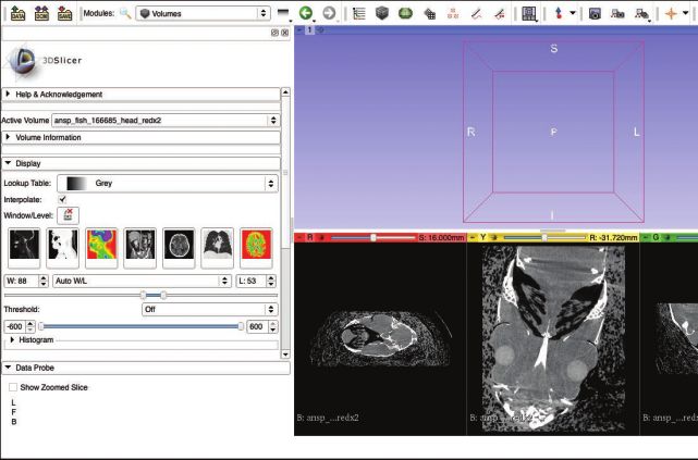
2 T. J. Buser et al.
ﻭﻥﺵﻡﻝ ﺃﻱﺽﺍ ﺕﻉﻝﻱﻡﺍﺕ.ﺍﻝﺃﺏﻉﺍﺩ ﺭﻕﻡﻱﺓ ﻝﻝﻩﻱﺍﻙﻝ ﺍﻝﺕﺵﺭﻱﺡﻱﺓ
ﺡﻭﻝ ﺍﻝﺕﺵﺭﻱﺡ ﺍﻝﻡﺡﻭﺱﺏ ﻭﺕﻕﻝﻱﺹ ﺍﻝﺏﻱﺍﻥﺍﺕ ﻭﺕﺹﺩﻱﺭﻩﺍ
ﻝﻝﺍﺱﺕﺥﺩﺍﻡ ﻑﻱ ﺕﻁﺏﻱﻕﺍﺕ ﻥﻩﺍﺉﻱﺓ ﻡﺙﻝ ﺍﻝﻁﺏﺍﻉﺓ ﺙﻝﺍﺙﻱﺓ
ﻥﻕﺩﻡ ﻡﻕﺍﻁﻉ ﻑﻱﺩﻱﻭ ﺕﻙﻡﻱﻝﻱﺓ ﻭﻡﺱﺍﺭﺍﺕ ﻉﻡﻝ، ﺃﺥﻱﺭﺍ.ﺍﻝﺃﺏﻉﺍﺩ
:ﻝﺕﻭﺽﻱﺡ ﻙﻱﻑ ﺕﺏﺱﻁ ﺍﻝﺇﺝﺭﺍﺀﺍﺕ ﺥﻡﺱ ﺍﺱﺕﺥﺩﺍﻡﺍﺕ ﻡﺡﺩﺩﺓ
ﻭﻉﺯﻝ،ﻕﻱﺍﺱ ﺍﻝﺱﻡﺍﺕ ﺍﻝﻭﻅﻱﻑﻱﺓ ﺍﻝﻡﺭﺕﺏﻁﺓ ﺏﺍﻝﺕﻍﺫﻱﺓ
ﻭﻉﺯﻝ ﺍﻝﻡﻥﺍﻁﻕ ﺫﺍﺕ ﺍﻝﺍﻩﺕﻡﺍﻡ،ﺍﻝﻩﻱﺍﻙﻝ ﺍﻝﺕﺵﺭﻱﺡﻱﺓ ﺭﻕﻡﻱﺍ
ﻭﺝﻡﻉ ﺍﻝﺏﻱﺍﻥﺍﺕ،ﺏﺍﺱﺕﺥﺩﺍﻡ ﺍﻝﺕﻕﻁﻱﻉ ﺵﺏﻩ ﺍﻝﺁﻝﻱ
ﻭﺕﻕﻝﻱﺹ ﺡﺝﻡ ﺍﻝﻡﻝﻑ،ﺏﺍﺱﺕﺥﺩﺍﻡ ﺃﺩﻭﺍﺕ ﺏﺹﺭﻱﺓ ﺏﺱﻱﻁﺓ
.ﻭﺕﺡﻭﻱﻝﻩ ﻝﻥﻡﻭﺫﺝ ﺙﻝﺍﺙﻱ ﺍﻝﺃﺏﻉﺍﺩ
Introduction 2019), these repositories encourage data reuse, rean-
Downloaded from https://academic.oup.com/iob/article/2/1/obaa009/5818881 by guest on 15 October 2020
The applications of three-dimensional (3D) visual- alysis, and reinterpretation, and have ushered in a
izations of internal anatomy are varied and vast, digital renaissance of comparative morphology.
spanning a galaxy of analytical possibilities. Most of the 3D images in the online digital librar-
Recently, the increased ease of gathering such data ies result from computed tomography scanning,
has led to their widespread adoption in the compar- commonly known as ‘‘CT’’ or ‘‘cat’’ scanning, which
ative morphological community. The embrace of this benefits from the quadruple advantages of non-
new data type has, in turn, catalyzed many recent destructivity, shareability, printability, and afford-
biological discoveries, such as revealing brain and ability (Cunningham et al. 2014; Sutton et al.
muscle activity during bird flight (positron emission 2014). CT scanning neither invades, modifies, or
tomography scanning; Gold et al. 2016), determining destroys the original sample. The digital nature of
how blood circulates through vasculature (magnetic CT data makes it easy to share via open-access plat-
resonance imaging; O’Brien and Williams 2014; forms and has sparked ‘‘big data’’ initiatives, such as
O’Brien 2017), revealing the function of the appen- oVert (floridamuseum.ufl.edu/overt) and the
dicular skeleton during locomotion and feeding in #ScanAllFishes projects (adamsummers.org/scanall-
live sharks (X-ray Reconstruction of Moving fish). The simplicity of converting CT scans to digital
Morphology, 3D fluoroscopy coupled with com- ‘‘surfaces’’ allows almost any anatomical structure to
puted tomographic [CT] animation; Camp et al. be 3D printed, even permitting structures to be ar-
2017; Scott et al. 2019) and reconstructing the feed- tificially warped, scaled, or mirrored to fit experi-
ing behavior of long-extinct monsters of the deep mental or teaching needs (Stayton 2009). Scans can
(CT imaging of Helicoprion; Tapanila et al. 2013). also be converted into digital ‘‘meshes’’ which can be
Other researchers have used 3D digitization to edu- used to gather 3D geometric morphometrics data
cate and inform. Anatomical models of living and (Lawing and Polly 2010), model the reaction forces
extinct taxa can be built digitally so that students on the structures using finite element analysis (FEA;
can manipulate, dissect, and scale anatomical struc- see Hulsey et al. 2008), predict fluid flow around
tures online (see Rahman et al. 2012; Manzano et al. structures using computational fluid dynamics (see
2015), used to make 3D prints of missing bones of Inthavong et al. 2009), study multibody dynamics
incomplete physical specimens, or print whole rare (Lautenschlager et al. 2016), or render and animate
or otherwise difficult to acquire specimens for use in 3D objects (Garwood and Dunlop 2014).
teaching comparative anatomy (Gidmark 2019; Staab Perhaps most importantly, the decreasing cost,
2019). For example, the anatomically accurate, 3D size, and complexity of CT hardware, and the devel-
printed, vertebrate skull magnetic puzzles by Singh opment of open source software like Horos (https://
et al. (2019) allow students to understand how dif- horosproject.org/) or 3D Slicer (Fedorov et al. 2012;
ferent parts of the skull fit together. Kikinis et al. 2014, https:// download. slicer. org) has
Open source efforts like MorphoSource (Boyer opened access to scientists working outside the bio-
et al. 2016; morphosource.org) and DigiMorph (dig- medical arena. Aspiring digital anatomists no longer
imorph.org) aggregate thousands of digital 3D mod- need to seek time on the multi-million-dollar, room-
els into anatomical libraries and serve them freely to sized set-ups in hospitals, but can use desktop
researchers, teachers, and laypersons alike. Like other machines costing far less. The spread of these smaller
synthetic, open access approaches to data manage- systems, often purchased through collaborative inter-
ment and data sharing (Sidlauskas et al. 2009; departmental funding opportunities, has drastically
Whitlock 2011; but see also Hipsley and Sherratt decreased the cost per study, increased the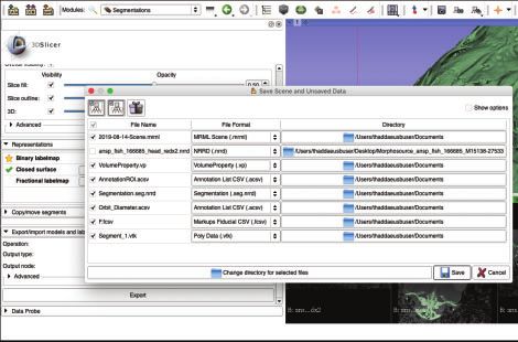
Guide to the CT galaxy 3
willingness of researchers to share their data, and more reasonable for older/slower machines, although
caused CT data to explode in popularity, even most any reasonably up-to-date machines (e.g., Mac
among scientists who lack access to CT hardware OS X Lion 10.7.3, Windows 7, Ubuntu 10.10, or
(see Davies et al. 2017). The methods have now newer) can perform all manipulations and analyses
transcended biomedical and anthropological research herein.
to penetrate fields like organismal taxonomy, pale-
ontology, comparative anatomy, and physiology, as
well as biomechanics and biomimetics (Cohen et al. Software
2018; Divi et al. 2018; Santana 2018; Rutledge et al. This workflow is designed to be completely open to
2019). The advantages of biodiversity and taxonom- any researcher, educator, or enthusiast. Generally
ical research cannot be understated as rare, endemic, speaking, the only limitation is access to a computer
and understudied taxa can now be shared widely. with at least 8 GB of random access memory (RAM),
Downloaded from https://academic.oup.com/iob/article/2/1/obaa009/5818881 by guest on 15 October 2020
More open access to specimens allows for systematic though this depends mostly on the size of the file to
hypotheses to be updated, re-examined, and repli- be analyzed. For optimal performance, we recom-
cated, and each scan preserves an in silico virtual mend that the data file not exceed one-tenth to
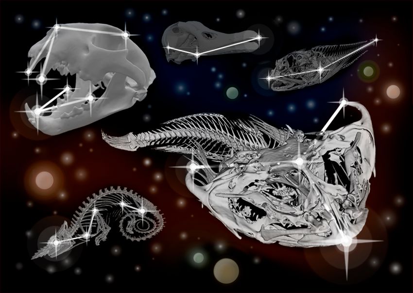
record of morphology for posterity. Metaphorically, one-fourth the size of the available RAM on your
each of these virtual specimens can be considered a computer. For example, if you have 8 GB of RAM,
point of light in a vast and growing constellation your data file should be no larger than 0.8 GB (800
depicting the world’s biological diversity. Those MB) to 2 GB. If the file that you intend to analyze is
researchers able to navigate that starfield, which we larger than this range, we include a variety of steps
dub the CT galaxy, will be poised to visualize and below for down-sampling or working around the
analyze biodiversity in ways never before possible. computationally and/or memory-intensive steps of
As is typical when technologies become newly af- CT analysis. There are a variety of software programs
fordable and accessible, the pace of method develop- available to process CT data, and the programs we
ment has far outstripped the pace of training. employ are freely available and cross-platform
Though many researchers and educators have be- (Table 1; see also Abel et al. 2012). Before beginning
come aware of CT’s potential, relatively few have the workflow, ensure that you have installed the lat-
been able to participate in focused training work- est stable version of the ImageJ (Schneider et al.
shops. Strides have been made in establishing best 2012; Rueden et al. 2017) expansion Fiji
practices in the process of CT scanning itself, and (Schindelin et al. 2012, https:// fiji. sc; we use
in the curation of 3D data (Davies et al. 2017; ImageJ v2.0.0 herein) and 3D Slicer (https:// down-
Keklikoglou et al. 2019). However, the only available load. slicer. org; v.4.10.2 used herein). We also rec-
training protocols for analyzing the CT data after ommend that users interested in working with 3D
they have been gathered have been ad hoc efforts surface meshes install MeshLab (Cignoni et al. 2008;
developed within research groups and passed among Pietroni et al. 2010, www. meshlab. net; v. 2016.12
scientists via email and similar channels. This con- used herein). If your computer has a dedicated
tribution aims to democratize access to such training graphics card, you can use it in Slicer to reduce
by publishing an open-access workflow using freely lag time when rendering your data in 3D. The pro-
available and cross-platform software. cess for telling Slicer to use your graphics card will
Herein, we outline a set of practices in the pro- vary based on your machine, operating system, and
duction, visualization, and analysis of CT data. We the brand of card. Generally, there will be an option
have found this workflow saves time and money in the automatically installed graphics card software
while maximizing efficiency. We hope that these sug- (NVIDIA—NVIDIA Control Panel, AMD—AMD
TM
gestions tempt the uninitiated to experiment with Catalyst Control Center, etc.) to select which pro-
CT methods for the first time or ease the struggle grams you want to use the card by default. Set this
of learning new techniques. To that end, we focus on up before running Slicer (you will likely have to re-
those often-tedious nuances of data preparation, for- start your machine). Alternatively, users can manu-
matting, and navigating software that commonly ally designate the graphics card within Slicer in the
hinder progress in CT-based studies of anatomy, volume rendering step (see Step 7.a.ii.1, below), but
functional morphology, and macroevolution. We this action must be repeated in every session. Finally,
also emphasize tools useful for creating pedagogical ensure that there is adequate hard drive space on
aids such as 3D prints and images of anatomical your machine for storing the CT dataset and deriv-
structures. Whenever possible, we include steps for ative products thereof. Approximately 10 GB will be
data-reduction that help to make processing time adequate for all steps involved in this workflow using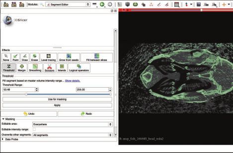
4                                                                                                                             T. J. Buser et al.

Table 1 Open-source, cross-platform software for visualizing and analyzing CT data

                                                      Operating
Software                          URL                 system(s)         Recommended uses; advantages                       Limitations
Drishti            https://github.com/nci/drishti   All (Windows,    Tools for image viewing, editing, proc-      Computationally demanding
                                                      Mac     OS,      essing, surface and volume rendering,       for volume rendering
                                                      Linux)           mesh generation, animation; intuitive
                                                                       user interface
SPIERS             https://spiers-software.org/     All              Tools for slice registration, image view-    Three separate modules for
                                                                       ing, editing, processing, surface ren-       aligning, editing, and view-
                                                                       dering, mesh generation, animation;          ing; only produces meshes
                                                                       handles large datasets well even on
                                                                       older/slower machines

                                                                                                                                                   Downloaded from https://academic.oup.com/iob/article/2/1/obaa009/5818881 by guest on 15 October 2020
Blender            https://www.blender.org/         All              Tools for editing 3D meshes, animation,      Lacks tools for basic image
                                                                       video editing; intuitive user interface,     processing (requires 3D
                                                                       customizable                                 model)
MeshLab            http://www.meshlab.net/          All              Tools for editing, analyzing, and refining   All processes restricted to
                                                                       3D meshes                                    working with meshes
3D Slicer          https://www.slicer.org/          All              Tools for image viewing, editing, proc-      Works best      on machines
                                                                       essing, surface and volume rendering,       with faster   graphics proc-
                                                                       file manipulation; intuitive user inter-    essing; may   require down-
                                                                       face, extensible and customizable with      sampling of   data
                                                                       a wide number of available modules,
                                                                       actively supported and developed
FIJI               https://fiji.sc/                 All              Tools for image viewing, editing, proc-      Not the most intuitive inter-
                                                                       essing, surface and volume rendering,       face for new users; some
                                                                       file manipulation; extensible and cus-      plugins no longer actively
                                                                       tomizable via the large number of           supported/developed
                                                                       purpose-built plugins available
Biomedisa          https://biomedisa.de/            Not applicable   Semi-automated   segmentation,         in-   Interpolates segments be-
                                                     (browser-         browser viewer                               tween labeled slices (no
                                                     based)                                                         other image processing
                                                                                                                    features)
MITK Workbench     http://mitk.org/                 All              Tools for image viewing, editing, proc-      Interface may be challenging
                                                                       essing, surface and volume rendering,        for new users
                                                                       file manipulation, data management;
                                                                       customizable for developers
ITK-SNAP           http://www.itksnap.org/          All              Tools for manual and semi-automated          Features limited to those re-
                                                                       segmentation; easily navigable user          lated to segmentation
                                                                       interface
MANGO              http://ric.uthscsa.edu/mango/    All              Tools for image editing, processing, sur-    Interface may be challenging
                                                                       face and volume rendering, file manip-       for new users
                                                                       ulation; command line accessible,
                                                                       customizable for developers

the example datasets. Users who wish to store and                       manipulated to reduce file size before being exported
process several CT datasets should consider the size                    as a single file in Nearly Raw Raster Data (NRRD)
of the datasets with respect to their available hard                    format (Steps 2–4). The user then imports the file
drive space. Datasets available on MorphoSource                         into the program 3D Slicer, which can visualize the
range from 200 MB to 10 GB in size, and we rec-                        specimen(s) or region(s) of interest. Later steps dem-
ommend a storage capacity of several terabytes (TB)                     onstrate how to measure and landmark morpholo-
for users wishing to engage in extensive (i.e., high                    gies of interest, and/or export data for downstream
sample size) studies using CT data.                                     applications (Steps 5–8). Step 7.f. specifically outlines
                                                                        the necessary workflow for generating the 3D surface
Workflow                                                                renders for use in eventual 3D printing. The final
Figure 1 illustrates the steps of this workflow. Briefly,               step of the workflow (Step 9) presents five analytical
the user will acquire a tomographic dataset (Step 1)                    examples to launch the reader’s exploration of prac-
and read it into the program Fiji, where it can be                      tical applications.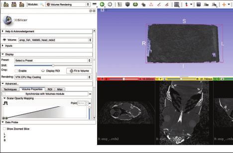
Guide to the CT galaxy                                                                                                       5

                   1. Acquire CT data from source
                                                                    working location (we recommend a local file loca-
                                                                    tion such as the desktop rather than a remote drive).
                                                                    If the image series is in any format other than
               2. Import tomographic dataset into Fiji              DICOM, locate the resolution/dimensionality data
                                                                    on either the data host website (Fig. 2A) or in the
                                                                    scanner log file. Note that MorphoSource removes
       3. Optional data preperation steps in Fiji, see Figure 3     the original scanner log file from their uploaded
                                                                    datasets, but the voxel dimensions can be found in
                                                                    the .CSV file accompanying your downloaded image
                                                                    stack dataset under the ‘‘x res,’’ ‘‘y res,’’ and ‘‘z res’’
           4. Export tomographic dataset as NRRD format
                                                                    columns. For the purposes of demonstrating the
                                                                    steps in our workflow, we will use a CT reconstruc-

                                                                                                                                  Downloaded from https://academic.oup.com/iob/article/2/1/obaa009/5818881 by guest on 15 October 2020
                5. Load NRRD volume into 3D Slicer                  tion of a pacu specimen (Pisces: Characiformes:
                                                                    Piaractus brachypomus; Academy of Natural
                                                                    Sciences of Drexel University, specimen ID: Fish:
                    6. Optimize density threshold                   166685), downloaded from MorphoSource.org
                                                                    (MorphoSource ID M15138-27533, see Fig. 2A and
                                                                    Supplementary Video S1). This is a modest-sized
      7. Optional data analysis steps in 3D Slicer, see Figure 11   dataset (2.5 GB) that works well on most
                                                                    machines. However, readers whose machines have
                                                                    low available RAM (i.e.,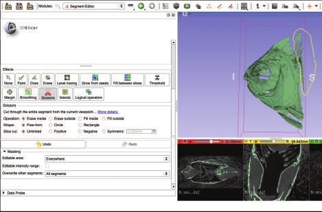
6                                                                                                                    T. J. Buser et al.

                                                                                                                                          Downloaded from https://academic.oup.com/iob/article/2/1/obaa009/5818881 by guest on 15 October 2020
                         A

                         B

Fig. 2 Acquiring CT data and loading them into the program Fiji. (A) The MorphoSource webpage (MorphoSource ID 15138) for a
pacu (P. brachypomus) specimen from the Academy of Natural Sciences of Drexel University (specimen ID: Fish: 166685). The
downloadable CT image stack (MorphoSource ID M15138-27533) and the specimen resolution data are each highlighted with a red
box. (B) The image stack from (A) being imported into Fiji, with the recommended import options highlighted in red boxes. Illustrates
Workflow Step 2.

(a) Open Fiji, go to ‘‘File,’’ then ‘‘Import,’’ and se-                 (ii) Note: The use of the virtual stack reduces the
     lect ‘‘Image sequence.’’                                                time it takes to read-in the dataset, and we
(b) Navigate to the folder containing your tomo-                             have found this helpful in saving time when
     graphic image stack and select the folder                               cropping images. However, advanced users
     (Mac) or any image within the folder                                    may wish to adjust parameters of the images
     (Windows), and press ‘‘Open.’’                                          (e.g., brightness and contrast) in Fiji. These
                                                                             steps are beyond the scope of this workflow,
(c) Next, Fiji will present you with a window of
                                                                             but for such users, we do not recommend
     ‘‘Sequence Options,’’ where you can customize
                                                                             using the virtual stack option, as this can
     your import. If they are not checked already,
                                                                             introduce system errors when attempting to
     check the box for ‘‘Sort names numerically’’
                                                                             modify the image parameters of large data-
     and ‘‘Use virtual stack.’’ Ensure that the
                                                                             sets. For these advanced users, or users
     ‘‘Increment:’’ is set to ‘‘1’’ and that the ‘‘Scale:’’
                                                                             attempting to analyze datasets with file sizes
     percent is set to ‘‘100.’’ Press ‘‘OK’’ (Fig. 2B).
                                                                             larger than the available memory (RAM) on
    (i) Note: If desired, it is possible to reduce the
                                                                             their computer, Supplementary Script S1 will
         file size of your stack through down-
                                                                             enable FIJI to crop and/or adjust image
         sampling, but do not attempt to do so
                                                                             parameters of image sequences with large
         here. See Step 3.e below.
                                                                             file sizes.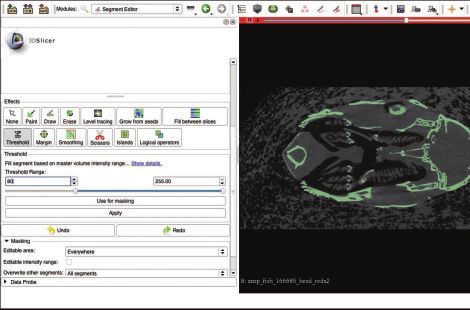
Guide to the CT galaxy                                                                                                                  7

                        2. Import tomographic dataset
                                                                                          may be indicated in the specimen data
                                                                                          (Fig. 2A).
                                                                                     (ii) If necessary, convert the units so that a sin-
                        Need to measure length?     YES
                                                             3a. [Optional]
                                                                                          gle number is present on the left side of the
                                                             Specify voxel                decimal place. For example, if the pixel size
                                       NO                    size
                                                                                          is reported as 39.989574 mm, convert it an
                        YES    Only interested in one area                                arbitrary unit that represents 107 m. For
  3b. [Optional]               of long axis of specimen
  Digitally isolate
                               (e.g., head)?
                                                                                          our example analysis, we will refer to this
  specimen in
  z-dimension
                                                                                          unit as a ‘‘pym,’’ and the pixel size of the
                                       NO
                                                                                          above example would be 3.9989574 pym.
                                                                                          The voxel dimensions for the pacu specimen

                                                                                                                                             Downloaded from https://academic.oup.com/iob/article/2/1/obaa009/5818881 by guest on 15 October 2020
                      Only interested in one area   YES
                                                             3c. [Optional]
                                                                                          are given as 0.04 mm (Fig. 2A), so would be
                      of wide axis of specimen
                      (e.g., single bone)?                   Digitally isolate            represented as 4 pym. The pixel size of the
                                                             specimen in
                                                             x,y-dimension                sculpin reconstruction is ‘‘0.0299 mm’’ and
                                       NO                                                 we would represent this as 2.99 pym. This
                                                                                          step is critical for avoiding arbitrary scaling
                               Want to visualize the 3D
 3d. [Optional]
                        YES
                               structure of your specimen?
                                                                                          and rounding issues in 3D Slicer, especially
 3D volume                                                                                for users working without a dedicated
 rendering
                                       NO
                                                                                          graphics card in their machine.
                                                                                    (iii) In Fiji, click on the window that contains
                                                    YES
                           File size > 2GB?                  3e. [Optional]               the image stack data that you opened in
                                                             Reduce the file
                                                             size of your                 Step 2.
                                                             dataset
                                       NO                                                (1) Go to: ‘‘Image,’’ then select ‘‘Properties.’’
                                                                                         (2) In the window that opens, change the
              4. Export tomographic dataset as NRRD format                                    ‘‘Unit of length’’ to whichever is most
                                                                                              appropriate for your data (e.g., pym),
Fig. 3 Decision tree for Workflow Steps 2–4, all performed in                                 and change the pixel/voxel dimensions
the using the program Fiji, which is an extension of the program                              to the appropriate dimension of your
ImageJ. Follow the decision tree to determine which options in                                data. Press ‘‘OK’’ (Fig. 4).
Step 3 may be useful for your dataset and intended analyses.

                                                                                 (b) Digitally isolate your specimen/area of interest
3. Optional steps—data preparation                                                    in the z-dimension: For use when working with
There are several optional steps available within Fiji                                a large volume of data and/or when you are
that serve to prepare the data for analysis in 3D                                     interested in only a portion of your CT dataset
Slicer. Use the decision tree illustrated in Fig. 3 to                                (e.g., you are interested in only skull but have
decide which (if any) optional steps are appropriate                                  scan data for the entire skeleton). This step
for your dataset and your intended analyses thereof.                                  helps reduce file sizes and increases processing
                                                                                      speed.
(a) Specify voxel size: For use when any of your
                                                                                     (i) Locate the upper and lower bounds of your
    downstream analyses may include length. This
                                                                                           area of interest in the z-dimension by scroll-
    step is highly recommended. Note: this step is
                                                                                           ing through the image stack using the scrub
    usually not necessary if your tomographic data-
                                                                                           bar at the bottom of your image stack win-
    set is in DICOM format.
                                                                                           dow (Fig. 5A).
    (i) Locate the x, y, and z-dimension length of                                   (ii) Record the image number for each bound
        your tomographic dataset. If your data come                                         (Fig. 5A and B).
        from the output of a CT reconstruction, the                                  (iii) Create a substack of just the images that
        voxel/pixel size is indicated in the log file of                                     contain your region of interest.
        the reconstruction (e.g., ‘‘Image Pixel Size                                     (1) Go to: ‘‘Image,’’ then ‘‘Stacks,’’ then
        (um)¼39.989574’’; in this case, it is implicit                                        ‘‘Tools,’’ and select ‘‘Make Substack ’’
        that this is the length of each dimension). If                               (iv) In the ‘‘Substack Maker’’ window that pops up,
        your data come from an online repository                                            input the range of images that contain your
        such as MorphoSource.org, this information                                          region of interest and press ‘‘OK’’ (Fig. 5C).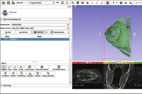
8                                                                                                                     T. J. Buser et al.

                         A

                                                                                                                                           Downloaded from https://academic.oup.com/iob/article/2/1/obaa009/5818881 by guest on 15 October 2020
                         B

Fig. 4 Specifying voxel size for the CT image stack from Workflow Step 1 using the program Fiji. The default dimensional data and unit
of length (A) are replaced with the values indicated on the MorphoSource web page shown in Step 2.a that have been converted to
units of ‘‘pym’’ (B). See text for details. Illustrates Workflow Step 3.a.

    (v) The substack that you specified will open in a                       (1) Use the rectangle tool on any image in
           new stacks window titled ‘‘Substack’’ followed                        your image sequence that contains your
           by the range that you specified in parentheses.                       specimen (Fig. 6B).
    (vi) Use this window for all additional steps.                           (2) Use the scroll bar at the bottom of the
        (1) Note: It may help to close the original                              window to visually check all images that
              stack window to avoid confusion, though                            contain your specimen to ensure that
              leaving it open is mostly harmless.                                your highlighted region is not too large
        (2) Note: If attempting to analyze a dataset                             or too small (Fig. 6C).
              whose file size is larger than your avail-                        (a) Adjust borders of your rectangle as
              able RAM, see Workflow Step 2.c.ii.                                   necessary.
(c) Digitally isolate your specimen/area of interest                    (iii) Crop the image stack to eliminate all the
     in the x, y-dimension: For use when working                               area outside of your rectangle.
     with a large volume of data and you are inter-                         (1) Go to ‘‘Image,’’ and select ‘‘Crop.’’
     ested in only a portion of your CT dataset (e.g.,                      (2) Note: If attempting to analyze a dataset
     you are interested in only a single side of a bi-                           whose file size is larger than your avail-
     laterally symmetric structure such as the cra-                              able RAM, see Workflow Step 2.c.ii.
     nium). This step may prove ineffective for                     (d) Examine the 3D volume of your cropped im-
     highly 3D (e.g., coiled, spiraled) specimens, and                   age stack: Use this step to visualize the 3D
     user discretion is warranted in such instances.                     structure(s) contained within your image stack.
    (i) Select the ‘‘Rectangle’’ tool from the ‘‘(Fiji Is                This is useful for verifying that any previous
          Just) ImageJ’’ toolbar (Fig. 6A).                              digital dissection did not unintentionally remove
    (ii) Use the rectangle tool to select an area of                     any anatomical structures of interest. This step
           your scan that encompasses all of your                        uses the ‘‘3D Viewer’’ plugin (Schmid et al.
           specimen/area of interest.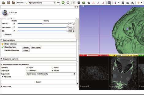
Guide to the CT galaxy                                                                                                                   9

  A                                                                         A

                                                                                                                                              Downloaded from https://academic.oup.com/iob/article/2/1/obaa009/5818881 by guest on 15 October 2020
  B
                                                                            B

  C
                                                                            C
Fig. 5 Digital isolation in the z-dimension on the image stack
from Workflow Step 1. The scrub bar is highlighted with a red
                                                                          Fig. 6 Digital isolation in the x, y-dimension of the image stack
box in (A and B). The upper bounds of the region of interest is
                                                                          from Workflow Step 3.b. The rectangle tool (A) is used to en-
indicated on the scrub bar with a red arrow in (A), the lower
                                                                          compass the region of interest (in yellow) (B, C). The scrub bar
bounds of the region of interest is indicated with a red arrow on
                                                                          is highlighted in a red box and is used to locate the upper (B)
the scrub bar in (B). The image number corresponding to the
                                                                          and lower (C) bounds of the region of interest (denoted with red
upper and lower bounds is highlighted with a red box in (A and
                                                                          arrowhead). Illustrates Workflow Step 3.c.
B) (respectively). The image range containing the region of in-
terest is specified in the ‘‘Slices:’’ range and highlighted with a red
box in (C). Illustrates Workflow Step 3.b.                                       (2) Go to ‘‘Edit,’’ and select ‘‘Adjust
                                                                                       threshold.’’
                                                                                 (3) Slide the ‘‘Threshold:’’ scroll bar until the
     2010), which comes pre-loaded in the Fiji soft-                                   rendering highlights the material with the
     ware package.                                                                     density of your choice (Fig. 7B and C).
 (i) Go to ‘‘Plugins,’’ and select ‘‘3D Viewer.’’                                (4) Press ‘‘OK.’’
 (ii) Optional: Change the ‘‘Resampling factor:’’                          (iv) Note: The volume rendering is a rotatable 3D
       from the default value of ‘‘2’’ to a higher num-                         area. Users with Microsoft Windows operating
       ber (e.g., 8) to decrease the amount of time                            systems have reported issues with the rotation
       it will take your computer to load the 3D vol-                           axis of the 3D volume in the ImageJ 3D
       ume rendering (Fig. 7A).                                                 Viewer. Until these issues are resolved by
         (1) Note: This step will decrease the resolu-                          developers, Windows users can get around
             tion of the rendering but will not affect                          this issue by grabbing with the mouse within
             the underlying slice data.                                         the ImageJ 3D Viewer window but outside of
 (iii) Optional: Change the threshold value for the                             the 3D volume bounding box to rotate the area
        opacity of the volume rendering to highlight                            (i.e., click and drag in the black space sur-
        the denser materials (e.g., bone) in your scan.                         rounding the bounding box to properly rotate
         (1) Select the ‘‘ImageJ 3D Viewer’’ window.                            the area within the bounding box).
10 T. J. Buser et al.
A
A
Downloaded from https://academic.oup.com/iob/article/2/1/obaa009/5818881 by guest on 15 October 2020
B
Fig. 8 Reducing the file size of the dataset using a reduction
B factor applied to the image stack from Workflow Step 1. The
initial file size and the reduction factor are each highlighted with
a red box in (A). The resulting file size from applying the re-
duction factor is highlighted with a red box in (B). Illustrates
Workflow Step 3.e.
can produce 3D models without loading the
data into memory.
(i) The file size of your current image stack is indi-
cated at the top of the stack window (Fig. 8A).
(ii) To reduce the size, go to ‘‘Image,’’ then
C ‘‘Stacks,’’ then ‘‘Tools,’’ and select ‘‘Reduce ’’
(iii) The default reduction factor is ‘‘2’’ (Fig. 8A),
Fig. 7 Visualization of CT data with a 3D volume rendering of this reduces the number of slices and the size
the image stack from Workflow Step 3.c. The resampling factor of your dataset by half and any single voxel in
(A) does not modify the underlying image data but decreases the the new dataset will comprise the average
resolution of the visualization in order to reduce loading time.
value of a 2 2 2 cube of voxels in the
We recommend a resampling factor of between 2 (small datasets
and/or fast computer hardware) and 10 (large datasets and/or
original dataset.
slow computer hardware). Adjust the threshold from its initial (1) Tip: Simply divide the current file size of
value (B) until the anatomy of interest is clearly visible (C). your dataset by the target file size to cal-
Illustrates Workflow Step 3.d. culate the reduction factor. For example,
if your current file size is 4.5 GB, and
your target size is 1.5 GB, use a reduction
(e) Reduce the file size of your image stack by factor of ‘‘3.’’
down-sampling: This step maintains the dimen- (iv) When the reduction process is complete, the
sionality of your specimen but reduces the res- new number of slices and the new file size
olution and thereby file size of the data. This will replace the old values at the top of the
can affect the visualization of minute structures stack window (Fig. 8B).
on your specimen but may be necessary for (v) Note: if you did NOT set the dimensionality
downstream processing in programs that strug- data for voxel size (i.e., Step 3.a above),
gle with large file sizes (e.g., file sizes >2GB will your voxel dimensions will be given in
crash 3D Slicer on most computers with 8GB ‘‘pixels’’ by default and you will need to
of RAM). Advanced users working with large file manually change the voxel depth for your
sizes (or limited RAM) are encouraged to ex- image stack after the reduction process is
plore the program SPIERS (see Table 1), which complete.Guide to the CT galaxy 11
Downloaded from https://academic.oup.com/iob/article/2/1/obaa009/5818881 by guest on 15 October 2020
A
B
Fig. 9 Loading image stack data into 3D Slicer. Use the drop-down menus to navigate the various modules and workspace views
available in 3D Slicer (A). (B) The NRRD format tomographic dataset from Step 4 successfully loaded into 3D Slicer. Illustrates
Workflow Step 5.
(1) Go to: Image ! Properties. (a) Click on ‘‘Choose File(s) to Add.’’
(a) Change ‘‘Voxel depth:’’ to whatever (b) Navigate to the NRRD file.
number you used as your reduction
(c) Press ‘‘OK’’ and the NRRD will load.
factor. For example, if you used a re-
duction factor of ‘‘3,’’ change the (d) Ensure that the display is set to conventional:
voxel depth to ‘‘3.’’ (i) Click the ‘‘Workspace view’’ button to reveal a
drop-down menu and select ‘‘Conventional’’
(b) Press ‘‘OK.’’
for optimal widescreen viewing (Fig. 9A).
4. Export the image stack as NRRD format
(e) Once the file has loaded, your screen should
(a) Go to ‘‘File,’’ then ‘‘Save As,’’ and select ‘‘Nrrd.’’ look something like Fig. 9B.
(b) Specify file name and location and press ‘‘Save.’’ (f) If you specified the voxel size of your data (Step
5. Load NRRD volume into 3D Slicer 3.a.), change the default unit of length in Slicer
to match the units of your data.
3D Slicer is set up such that different sets of related
(i) Click the ‘‘Edit’’ menu and select
tasks are grouped together in the ‘‘Modules:’’ drop-
‘‘Application Settings.’’
down menu. The program’s default module is called
(1) Select ‘‘Units’’ from the side menu.
‘‘Welcome to Slicer’’ and this is where the program
starts when it is first opened. In the ‘‘Welcome to (2) Check the box next to ‘‘Show advanced
Slicer’’ module, click on ‘‘Load Data’’ (Fig. 9A). options’’12 T. J. Buser et al.
Downloaded from https://academic.oup.com/iob/article/2/1/obaa009/5818881 by guest on 15 October 2020
A
B
Fig. 10 Image contrast optimization. The upper and lower bounds of the range of pixel values that will be displayed for the images in
the tomographic stack are indicated with red arrowheads in the starting (default) values (A) and after manual optimization (B).
Illustrates Workflow Step 6.
(3) Under the ‘‘Length’’ submenu, change 6. Optimize image contrast
the ‘‘Suffix’’ from the default value of This step adjusts the contrast of the image and is
‘‘mm’’ to the unit that you specified in useful for any downstream step where visually dif-
Step 3.a. (e.g., for our data, we would set ferentiating structures are useful, such as trimming
the suffix to ‘‘pym’’). and editing segmentations (e.g., Step 7.c). However,
(a) Note: We recommend users also it does not alter the underlying data; it simply alters
change the ‘‘Precision’’ level under how those data are visualized.
the ‘‘Length’’ submenu from its de-
fault value of ‘‘3’’ to a value of 5– (a) Click on the drop-down menu located in the
10. This will decrease errors and loss upper bar of the program window, to the right
of information due to rounding. of the word ‘‘Modules:’’
(i) Select ‘‘Volumes’’ module (Fig. 10A).
(4) Note: Users with a dedicated graphics card
can designate its use as a default setting here (b) Under the ‘‘Display’’ sub-menu there is a sliding
by selecting ‘‘Volume rendering’’ from the tool element, flanked by ‘‘W’’ and ‘‘L.’’
side menu, then changing the ‘‘Default ren- (i) Click the ‘‘Auto W/L’’ button (Fig. 10A) to
dering method:’’ to ‘‘VTK GPU Ray reveal a drop-down menu and select
Casting,’’ changing the ‘‘Default quality’’ to ‘‘Manual Min/Max.’’
‘‘Normal,’’ and changing the ‘‘GPU memory (c) Adjust the Min/Max slider bar maximum and
size’’ to match the GPU memory on their minimum (left and right pegs, respectively) to
machine. fine tune the contrast on your image slices.Guide to the CT galaxy 13
6. Optimize density threshold
measurements and landmark coordinate data directly
from the slices is a way to avoid the computation
and memory-taxing processes involved in 3D
Want to visualize the 3D YES
structure of your specimen? 7a. [Optional]
visualization.
Volume
rendering (a) Volume rendering: This step creates a 3D visu-
NO
alization of the dataset and allows the operator
7b. [Optional] YES Will you 3D print or conduct to assign different values of opacity and color to
Segment region further analyses outside of
of interest via Slicer?
materials of different density. It is useful for
density data exploration, measuring, and counting ana-
threshold
NO
tomical structures (see Step 7.d below), placing
anatomical landmarks (see Step 7.e below), and
Downloaded from https://academic.oup.com/iob/article/2/1/obaa009/5818881 by guest on 15 October 2020
Are you interested in only YES
7c. [Optional] creating images of the anatomy (see Step 7.a.ii.5
one area/structure within
your segmentation?
Isolate and
refine region
below; see also examples in Conway et al. 2017;
of interest Conway et al. 2018). Volume renderings have
NO been used to provide visual evidence of damage
or healing to parts of the skeleton (Kolmann et
YES Do you want to take
7d. [Optional]
measurements?
al. 2020), visualize otoliths (Paig-Tran et al.
Measure
anatomical 2016), assess stomach contents (Kolmann et al.
structure(s)
NO
2018), and track changes in the orientation of
anatomical structures across specimens
Are you interested in 3D YES
7e. [Optional] (Kolmann et al. 2016, 2019; see also Workflow
shape data for, e.g., 3D
geometric morphometrics?
Add markers to
anatomical
Step 9.d below). Volume renderings cannot be
structures used for 3D printing other downstream pro-
NO
cesses that take place outside of 3D Slicer such
YES Want to make a 3D model as FEA. Volume rendering can be computation-
7d. [Optional]
Export surface
for printing or further ally taxing, especially on older machines, and
/ 3D mesh analysis outside of slicer?
object
some users may experience frustrating lag-
NO times when attempting to visualize even
modest-sized datasets. If your machine has a
8. Save and/or export dedicated graphics card, using it will drastically
reduce lag and other difficulties associated with
Fig. 11 Decision tree for Workflow Steps 5–8, all performed volume rendering (see Step 7.a.ii.1 below).
using the program 3D Slicer. Follow the decision tree to deter- Alternatively, many of the same operations per-
mine which optional steps in Workflow Step 7 may be useful for formed on volume renderings (e.g., measuring
your intended analyses. anatomical structures) can be performed on sur-
face renderings (Step 7.b below), which do not
Adjust the maximum value so that the bone or tax the CPU nearly as much (but typically re-
other high-density material is clearly visible and quire more RAM than volume renderings in
distinct but that fine structures (e.g., sutures) Slicer).
are distinguishable and not washed-out by too (i) Click on the ‘‘modules’’ dropdown menu and
high of contrast. Adjust the minimum value so click on ‘‘Volume Rendering.’’
that the specimen is clearly distinct from the
(ii) In the ‘‘Volume Rendering Module,’’ tweak
background (see Fig. 10B).
the inputs until you can see the anatomical
7. Data visualization and analyses structures of interest (see Fig. 12):
There are many useful tasks and analyses available in (1) If you have a dedicated graphics card,
3D Slicer. Figure 11 illustrates a decision tree for change the rendering settings so that
selecting among the tasks that we have found to be Slicer uses the graphics card rather than
most common and useful. Many of the analyses your CPU to render your data. This will
within 3D Slicer can be performed directly on the increase the performance of your machine
tomographic image series or on a 3D visualization of drastically for all steps related to volume
the specimen(s) therein. For users with very limited rendering.
RAM and/or processing (i.e., Central Processing Unit (a) In the ‘‘Display’’ sub-menu, click the
[CPU]) speed, skipping Steps 7.a–7.c and taking dropdown menu titled ‘‘Rendering,’’14 T. J. Buser et al.
and change ‘‘VTK CPU Ray Casting’’
to ‘‘VTK GPU Ray Casting’’
(Fig. 12A).
(b) Expand the ‘‘Advanced ’’ sub-menu by
clicking on it (Fig. 12A).
(c) Click on the ‘‘Techniques’’ tab (Fig. 12B).
(i) Click on the ‘‘GPU memory size:’’
drop-down menu and select a unit
of memory that is close to but not
A
greater than that of your dedicated
graphics memory. For example, if
Downloaded from https://academic.oup.com/iob/article/2/1/obaa009/5818881 by guest on 15 October 2020
you have an ‘‘Intel Iris 1536 MB’’
graphics card, you would select ‘‘1.5
GB’’ from the drop-down menu
(Fig. 12B).
(d) Click on the ‘‘Quality:’’ drop down
menu and select ‘‘Normal’’ (Fig. 12B).
(i) Note: If you wish to take a high-
B quality snapshot of a volume render-
ing (see Step 7.a.ii.3 below), you can
avoid unnecessary lag time by opti-
mizing the volume rendering param-
eters under ‘‘Normal’’ quality, then
changing the quality to ‘‘Maximum’’
just before taking the snapshot.
(e) Note: The process for checking for the
presence and specifications of a dedi-
cated graphics card varies by operating
C
system, but this is a rigidly defined
area of doubt and uncertainty and
can typically be resolved with a quick
Internet search.
(2) Click the eyeball icon located to the left of
the ‘‘Volume’’ drop down menu (see
Fig. 12C) to toggle whether or not the
3D rendered volume is visible. If the eye
is closed, click it to open it and the vol-
ume will appear in the purple window
D (after some loading time).
(3) When your volume appears, it will show
Fig. 12 Basic volume rendering procedure. If your computer has
a dedicated graphics card, change the rendering settings to use it. up as a gray block in the purple window.
The ‘‘Rendering:’’ drop-down menu is highlighted in a red square Click the ‘‘Center View’’ button in the
(A), click it and select ‘‘VTK GPU Ray Casting.’’ The ‘‘Advanced ’’
sub-menu is highlighted in a red square (A). Click on it to ex-
pand. (B) The ‘‘Techniques’’ tab highlighted in a red square. In Fig. 12 Continued
that tab, change the ‘‘GPU memory size:’’ (highlighted in red box) Mapping’’ curve so that there are four points and they create a
to match the graphics memory of your computer and change the backwards ‘‘Z’’ shaped curve. Adjust the position of the second
‘‘Quality:’’ (highlighted in red box) to ‘‘Normal’’ (B). The eyeball point (indicated with a red arrow) until the anatomy of interest is
icon that toggles showing/hiding the volume rendering is visible, as shown in (C) (starting position) and (D) (final position).
highlighted with a red square (C). In the ‘‘Advanced ’’ submenu, Adjust additional volume rendering parameters in the
click the ‘‘Volume Properties’’ tab (highlighted in red box) (C). ‘‘Advanced’’ controls to fine-tune the visualization as needed.
Adjust the number and position of points on the ‘‘Scalar Opacity Illustrates Workflow Step 7.a i–iii.1.Guide to the CT galaxy 15
top-left of the purple window to center
the volume rendering (see Fig. 12C).
(4) For a quick visualization of the skeletons
of your specimen, click the ‘‘Preset:’’
drop-down menu.
(a) Hover your cursor over the top-left
image in the drop-down menu.
(i) The name ‘‘CT-AAA’’ will appear.
(b) Click this image.
A
(c) Located immediately below the ‘‘Preset:’’
drop-down menu is a slider bar for
Downloaded from https://academic.oup.com/iob/article/2/1/obaa009/5818881 by guest on 15 October 2020
adjusting the ‘‘Shift:’’ of the preset.
(i) Adjust the peg on the ‘‘Shift:’’ slider
bar left or right until the rendering
shows the skeleton of your specimen.
(5) For a customized visualization of your
specimen, click the ‘‘Volume Properties’’
tab in the ‘‘Advanced ’’ sub menu
(Fig. 12C).
B
(a) Adjust the ‘‘Scalar Opacity Mapping’’
controls to reveal the structure(s) of Fig. 13 Fine-tuning a volume rendering by adjusting the color
interest (Fig. 12C and D). rendering of the volume (A) and the background view settings
(i) Tip: Add points on the opacity value (B). Add and adjust the position of points (indicated with red
curve by clicking on it. Start with four arrows) in the Scalar Color Mapping graph and assign a color to
points. Select a point using the each point (A). In this example, there are five points. Points 1
‘‘Point:’’ box. Adjust the left-right po- and 2 are assigned the color black, Point 3 is assigned the color
sition (corresponds to the density/gray brown, and Points 4 and 5 are assigned the color white. The
view of the volume rendering in (B) has been adjusted such that
scale values of your original CT data-
the bounding box has been removed along with the axis labels,
set) of that point using the ‘‘X:’’ box. and the background color has been changed to ‘‘Black.’’ Illustrates
Adjust the opacity value of that point Workflow Step 7.a.iii.2.
using the ‘‘O:’’ box.
(ii) Tip: Start with four points in the Scalar color assignment screen. Select the
Opacity Mapping graph: two on the left color black and hit the ‘‘Okay’’ but-
at the bottom of the graph (O: 0.00) and ton), gold to the center, and white to
two on the right at the top of the graph (O: the right. Experiment with how
1.00). Adjust the X position of each point changing the position of the center
as follows: Point 0, X ¼ 0; Point 1, X ¼ 50; dot on the horizontal axis changes
Point 2: X ¼ 200; Point 3, X ¼ 255. Now, the color map on your specimen.
adjust the X position of Point 1 until the Try adding additional points by click-
structures of interest are revealed (Fig. 12C ing anywhere in the ‘‘Scalar Color
and D). Mapping:’’ graph. Experiment with
(b) Use the ‘‘Scalar Color Mapping’’ to different colors (and brightness values
assign colors to ranges of the opacity thereof) and positions for each dot
curve (Fig. 13A). until you find a scheme that you
(i) Tip: Start with three points: one on find suitable (see Fig. 13A).
the far left, one in the center, and (6) Tip: To further refine the 3D image,
one on the far right. Assign the color change the specimen view from
black to the far left (select the far-left ‘‘Conventional’’ to ‘‘3D Only’’
point, which should be point ‘‘0’’ in (Fig. 13A). Click the ‘‘Pin’’ button on
the ‘‘Point:’’ box and click the color the top left of the purple ‘‘3D Only’’ win-
box immediately to the right of the dow. Click the ‘‘Eye’’ button to open a
‘‘Point:’’ box. This will bring up the screen that allows you to toggle on and16 T. J. Buser et al.
off the specimen bounding box and 3D
axis labels (Fig. 13A). This screen also
allows you to change the background
color from ‘‘Light Blue’’ (default color),
to ‘‘Black’’ or ‘‘White.’’ There are many
other useful features contained in the
‘‘Pin’’ window. One of which is the blue
and red sunglasses button, which allows
the user to project the image using ana-
gram or other specialty-glasses-enabled A
schemes. When you are satisfied with
your view of the specimen, export an im-
Downloaded from https://academic.oup.com/iob/article/2/1/obaa009/5818881 by guest on 15 October 2020
age using the camera icon (Fig. 13B).
Your image will be saved by default at
the resolution of your screen. To change
the resolution of the image, change the
‘‘Scale factor:’’ to higher (increased reso-
lution) or lower (decreased resolution)
than the default value of ‘‘1.0.’’ When
you press ‘‘OK,’’ your image has been B
taken, but not yet saved. Go to the
‘‘File’’ drop-down menu and select
‘‘Save.’’ Here you can save your snapshot
by checking only the box for your labeled
snapshot (see Step 8 below).
(b) Segment bone or other dense material(s) of
interest using a density threshold: This step is
useful for creating 3D models of anatomy that
can be used for fine-scale digital dissection (see
Step 7.c), measuring (see Step 7.d), and/or plac- C
ing landmarks (see Step 7.e) on anatomical
structures. The segmentations produced in this Fig. 14 Creating a density-based segmentation of an anatomical
step can be used to create surface renderings structure of interest. Change the view (highlighted with a red
that can be exported as 3D meshes and used box in (A)) to ‘‘Red slice only’’ after adding a new segment and
for 3D printing and/or downstream analyses in clicking the ‘‘Threshold’’ button. Set the upper bounds of the
other programs (see Step 7.f). While we use a ‘‘Threshold Range’’ to a value of ‘‘255.’’ Adjust the lower bounds
density based ‘‘threshold’’ to create a segmenta- (indicated with a red arrow in (A and B)) so that only the ma-
terial of interest is highlighted. Too low of a value will capture
tion here, there are several other options within
extraneous material (B), but an appropriate value will capture
3D slicer for creating segmentations. We have only the material of interest (C). Illustrates Workflow Step 7.b.
found the threshold-based approach to be the
simplest and most accessible option, especially
(iii) Click the ‘‘Threshold’’ button (Fig. 14A).
for new users. However, we encourage readers
to explore the other options once they become (iv) Scroll down to find the ‘‘Threshold Range:’’
comfortable with the basic steps outlined here. indicator. You can adjust the lower and up-
(i) Click on the drop-down menu for per bounds of the threshold range by
‘‘Modules.’’ adjusting the left and right pegs (respec-
(1) Select ‘‘Segment Editor’’ module. tively) on the indicator bar, or by changing
the values in the left and right boxes (re-
(ii) Click the ‘‘Add’’ button to add a new seg-
spectively). For most applications (and/or
ment (Fig. 14A).
for a starting point), set the upper bounds
(1) Keep both the default color and name of
to the maximum value (255). Adjust the
this new segment or customize by double-
lower bounds according to the minimum
clicking on either one.Guide to the CT galaxy 17
density material that you wish to include in
your segment. Very low values of the lower
bounds will cause your segment to include
lower-density material while high values of
the lower bounds will result in only denser
material being included.
(1) Note: While most users working with
fresh or preserved specimens have little
need to adjust the upper bounds of the
threshold range beyond what is described A
above, users working with fossil data may
wish to adjust the upper threshold bounds
Downloaded from https://academic.oup.com/iob/article/2/1/obaa009/5818881 by guest on 15 October 2020
to eliminate undesirable high-density
materials in the surrounding matrix.
Users working with fossil data especially
are encouraged to review Sutton et al.
(2014).
(v) To get a closer look at the effect of changing
your threshold range, change the view of
your workspace so that you are only looking B
at one of the slice views of your data
(Fig. 14A). The default view is called Fig. 15 Isolating a region of interest from a segmentation. Using
‘‘Conventional’’ and includes a 3D window the 3D view of the segmentation (A), extraneous structures are
on top and a sagittal, coronal, and axial view selected and eliminated using the ‘‘Scissors’’ tool (B). Illustrates
below. Change the view to that of the sagit- Workflow Step 7.c.
tal slice (the red window below) by clicking
the Slicer layout button to reveal a drop-
it to your structure of interest (see Step 7.
down menu of different view options.
c below).
(1) Select ‘‘Red slice only’’ (Fig. 14B).
(vii) Press the ‘‘Apply’’ button (Fig. 14C).
(vi) Now we can clearly see the effects of chang-
ing our threshold range for this slice. Adjust (c) Isolate regions of interest from segmentation:
your threshold until as much of the bone is This step is useful for isolating small and/or
captured (it will change color to whatever complex structures such as individual bones
you have selected for your segment). from a skeleton, or a single specimen from
(1) Tip: Set your threshold value initially by scan data that contain multiple specimens.
lowering it until speckles of segment (as (i) Visualize the 3D structure of your segment.
indicated by the segmentation color) be- (1) Select ‘‘Conventional View’’ (Fig. 15A).
gin to appear in unwanted areas of your (2) In the ‘‘Segment Editor’’ module, click the
specimen (e.g., soft tissue such as the lens ‘‘Show 3D’’ button (Fig. 15A).
of the eye if present; see Fig. 14B). Next, (3) To reposition your specimen/segment in
raise the threshold value just until all of the 3D window, select the ‘‘None’’ tool
these undesirable spots disappear in the ‘‘Effects’’ section. Using your left
(Fig. 14C). Next, check for areas in your mouse button will rotate specimen, hold-
structure of interest that are thin and ad- ing down the ‘‘Shift’’ key while dragging
just the threshold as necessary to ensure with the left mouse button with reposi-
that all areas are encapsulated by the seg- tion your specimen, the right mouse but-
ment. It may not be possible to set a ton will zoom in and out.
threshold that perfectly captures your an-
(ii) Select the ‘‘Scissors’’ button in the ‘‘Effects’’
atomical feature of interest, but the seg-
section (Fig. 15B).
ment can be trimmed or expanded using
(1) This tool can be used on either the 3D
the eraser or paintbrush tools (respec-
view or any of the slice views and has
tively) to make fine adjustments to the
several options available, perhaps the
area included in the segment and matchYou can also read


