ParkNet: Drive-by Sensing of Road-Side Parking Statistics
←
→
Page content transcription
If your browser does not render page correctly, please read the page content below
ParkNet: Drive-by Sensing of Road-Side Parking Statistics
Suhas Mathur, Tong Jin, Nikhil Kasturirangan, Janani Chandrashekharan,
Wenzhi Xue, Marco Gruteser, Wade Trappe
WINLAB, Rutgers University, 671 Route 1 South, North Brunswick, NJ, USA
{suhas, tongjin, lihkin, janani, wenzhi, trappe, gruteser}@winlab.rutgers.edu
ABSTRACT
Urban street-parking availability statistics are challenging
to obtain in real-time but would greatly benefit society by
reducing traffic congestion. In this paper we present the de-
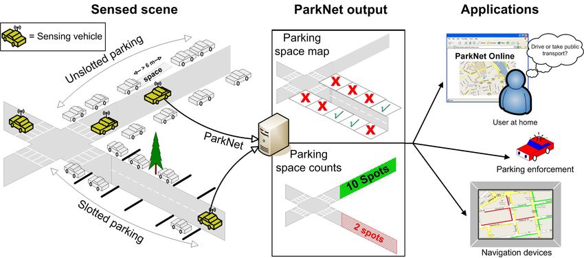
sign, implementation and evaluation of ParkNet, a mobile
system comprising vehicles that collect parking space occu-
pancy information while driving by. Each ParkNet vehicle
is equipped with a GPS receiver and a passenger-side-facing
ultrasonic rangefinder to determine parking spot occupancy.
The data is aggregated at a central server, which builds a
real-time map of parking availability and could provide this
information to clients that query the system in search of
parking. Creating a spot-accurate map of parking avail-
ability challenges GPS location accuracy limits. To address
this need, we have devised an environmental fingerprinting Figure 1: Categorization of urban sensing applica-
approach to achieve improved location accuracy. Based on tions by required location accuracy and relative dy-
500 miles of road-side parking data collected over 2 months, namics of the process being monitored.
we found that parking spot counts are 95% accurate and
occupancy maps can achieve over 90% accuracy. Finally,
we quantify the amount of sensors needed to provide ade-
in the form of 4.2 billion lost hours and 2.9 billion gallons of
quate coverage in a city. Using extensive GPS traces from
wasted gasoline in the United States alone. Several projects
over 500 San Francisco taxicabs, we show that if ParkNet
have recently sought to address this issue through the design
were deployed in city taxicabs, the resulting mobile sensors
of mobile systems that collect traffic congestion information
would provide adequate coverage and be more cost-effective
to improve route finding and trip planning [2, 3]. Unfortu-
by an estimated factor of roughly 10-15 when compared to
nately, a significant portion of traffic congestion is experi-
a sensor network with a dedicated sensor at every parking
enced in downtown areas where it is not always possible to
space, as is currently being tested in San Francisco.
reroute a driver. In these densely populated urban areas,
congestion and travel delays are also due to parking. In a
Categories and Subject Descriptors recent study [4], researchers found in one small business dis-
C.3 [Special-Purpose and Application-Based Systems]: trict of Los Angeles that, over the course of a year, vehicles
looking for parking created the equivalent of 38 trips around
General Terms the world, burning 47,000 gallons of gasoline and producing
730 tons of carbon dioxide. Clearly, addressing the problems
Algorithms, Design, Experimentaion, Measurement associated with parking in downtown areas would have sig-
nificant societal impact, both economically and ecologically.
1. INTRODUCTION Lack of information. One key factor contributing to ex-
Automotive traffic congestion imposes significant societal cess parking vehicle miles is a lack of information about road-
costs. One study [1] estimated a loss of $78 billion in 2007 side parking availability. While occupancy data for parking
garages is relatively straightforward to obtain through en-
try/exit counters, data is generally unavailable for road-side
parking. Detailed parking availability information would al-
Permission to make digital or hard copies of all or part of this work for low municipal governments to make better decisions about
personal or classroom use is granted without fee provided that copies are where to install parking meters and how to set prices. Don-
not made or distributed for profit or commercial advantage and that copies ald Shoup [5] has argued that road-side parking spots are
bear this notice and the full citation on the first page. To copy otherwise, to commonly underpriced compared to parking garages, and
republish, to post on servers or to redistribute to lists, requires prior specific that this fiscal consideration greatly exacerbates parking
permission and/or a fee.
MobiSys’10, June 15–18, 2010, San Francisco, California, USA. problems. Detailed information would allow travelers to ar-
Copyright 2010 ACM 978-1-60558-985-5/10/06 ...$5.00. rive at better decisions on mode of travel or use of parking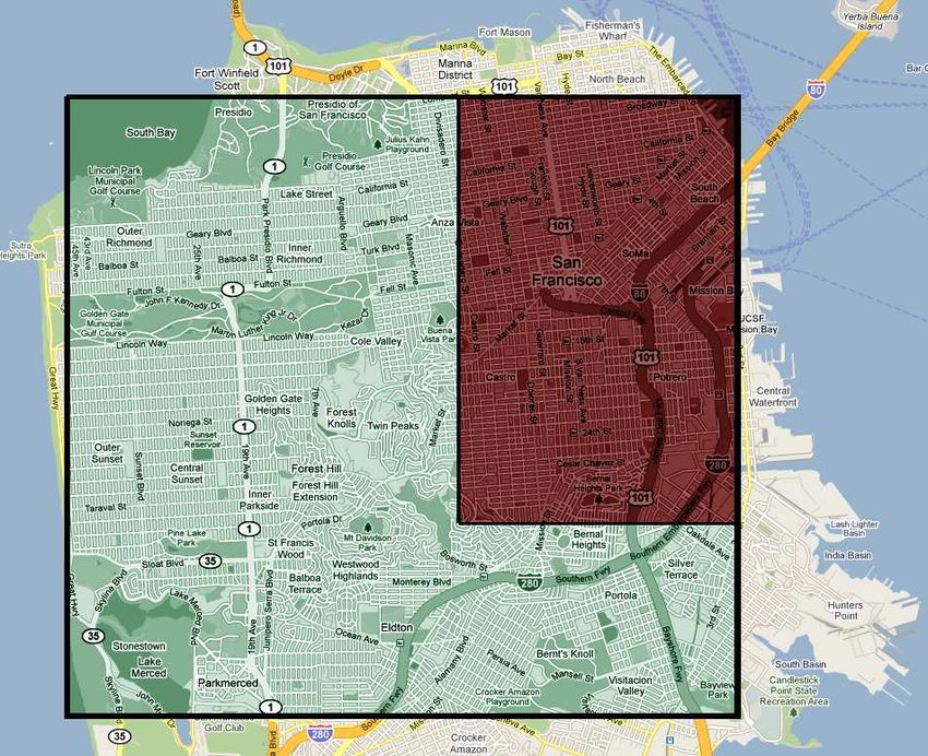
garages versus attempting road-side parking. Indeed, several
projects are already underway to monitor road-side park-
ing spaces by detecting the presence of parked vehicles over
parking spots using fixed sensors [6–8]. These efforts rely
on sensors installed into the asphalt or in parking meters.
This necessitates a large installation cost and operational
cost in order to adequately monitor the parking spaces at a
city-wide level, or even at the level of a downtown area. For
example, the SF-park project [8] aims to cover only 25% of        Figure 2: Ultrasonic sensor fitted on the side of a
the street parking spots in San Francisco, and will have a        car detects parked cars and vacant spaces.
cost of several million dollars. Unfortunately, even with such
a starting price tag, the cost of such a system does not scale
well with the number of parking spaces to be monitored,
and is also inherently limited to street-parking with clearly     buses, or parking enforcement vehicles. Further, we note
demarcated spaces. A further drawback of such systems is          that there is the potential to reuse ultrasonic rangefinders
that they require that wireless relay nodes be installed sepa-    already integrated in some modern vehicles for parking assist
rately on the road side (e.g. in lamp posts) in all areas where   and automated parking applications.
sensors are installed in the ground. However, projects such          Overview. In Section 2, we provide an overview of the
as [8] highlight the magnitude of the problem in large cities     challenges associated with identifying parking locations and
and the government’s dedication to long-term investments          their occupancy. In Section 3, we detail the system that we
in a smart parking infrastructure.                                have built for monitoring parking, providing the rationale
   Drive-by Parking Monitoring. In contrast to such               for the system choices that we have made. We next explore
fixed monitoring systems, this paper presents a mobile sys-       in Section 4 the ability of our system to monitor parking
tem that collects road-side parking availability information      spaces. Since one potential application we envision involves
at a lower cost. Our sensing platform consists of a low cost      associating cars with their specific, corresponding parking
ultrasonic sensor that simply reports the distance to the         slot, in Section 5 we next detail an approach to improve loca-
nearest obstacle and a GPS receiver that notes the corre-         tion accuracy sufficiently to support such an application. In
sponding location. Our sensor network leverages the mobil-        Section 6 we turn to exploring how many vehicles should be
ity of vehicles that regularly comb a city, such as taxicabs      part of such a mobile system in order to adequately monitor
and other government vehicles (parking enforcement, police        parking slots. We summarize the lessons learned in Section
cars, etc.) to reduce the number sensors needed. The cost         7 and place our work relative to related work in Section 8.
savings come from the fact that the status of parking spaces      Finally, we conclude the paper in Section 9.
in an urban area does not change very rapidly in time, and           In summary, the key contributions of this paper are:
hence continual sensing through fixed sensors is unneces-
                                                                     • Demonstrating the feasibility of a mobile sensing ap-
sary. Realizing this application, however, requires that sev-
                                                                       proach to road-side parking availability detection through
eral unique challenges in mobile systems be overcome that
                                                                       the design, implementation, and evaluation of such a
have not been addressed in prior efforts in mobile sensing.
                                                                       system. Our experimental evaluation uses over one
   In order to place our work in a broader context, consider
                                                                       month of data from up to three vehicles passing through
the diagram presented in Figure 1, where we have placed our
                                                                       the downtown Highland Park, NJ area;
ParkNet system relative to several notable vehicular monitor-
ing efforts in terms of the required location accuracy needed        • Proposing and evaluating an improved approach to
by the sensing application as well as the underlying rate of           GPS positioning using environmental fingerprinting that
change of the event being monitored. For example, in [9], a            allows us to achieve the location accuracies necessary
system is presented that monitors the presence of potholes             for precise matching of cars with their associated park-
in road surfaces. This involves monitoring a very slowly               ing slots;
changing quantity with moderate location precision. Traffic
monitoring systems, such as [2] on the other hand moni-              • Showing through trace-based simulations with a dataset
tor a more rapidly changing quantity, but require relatively           involving San Francisco taxis that a few hundred taxis
low precision. In contrast, ParkNet can be considered to re-           provide adequate spatio-temporal sampling of a down-
quire significant spatio-temporal accuracy as the occupancy            town area, which is precisely where parking is most
of parking spaces can vary on the order of minutes and, fur-           scarce.
ther, some applications in ParkNet might require significant
location accuracy in order to associate cars in specific park-    2. THE ROAD-SIDE PARKING CHALLENGE
ing slots.
                                                                     Finding street-side parking in a crowded urban area is a
   In our work, we have overcome the underlying challenges
                                                                  problematic task and one that most drivers dread. Finding
of dynamics and location accuracy associated with parking
                                                                  a parking space near one’s destination could be much easier
monitoring applications, through the careful integration of
                                                                  if there were a way to know ahead of time which areas have
ultrasonic measurements with GPS readings that are cor-
                                                                  available parking spaces. Often times, a street only a few
rected through environmental fingerprinting. Our ParkNet
                                                                  blocks away might have vacant parking spaces but a driver
system has been tested experimentally, collecting over 500
                                                                  looking for parking has no way of knowing this.
miles of road-side parking data over two months, and our
                                                                     One approach to addressing the road-side parking problem
results show that such a system could be fitted into vehicles
                                                                  may be a spot reservation system that allows vehicles claim
that frequently roam downtown areas, such as taxicabs, city
                                                                  available spots before they arrive at their destination. This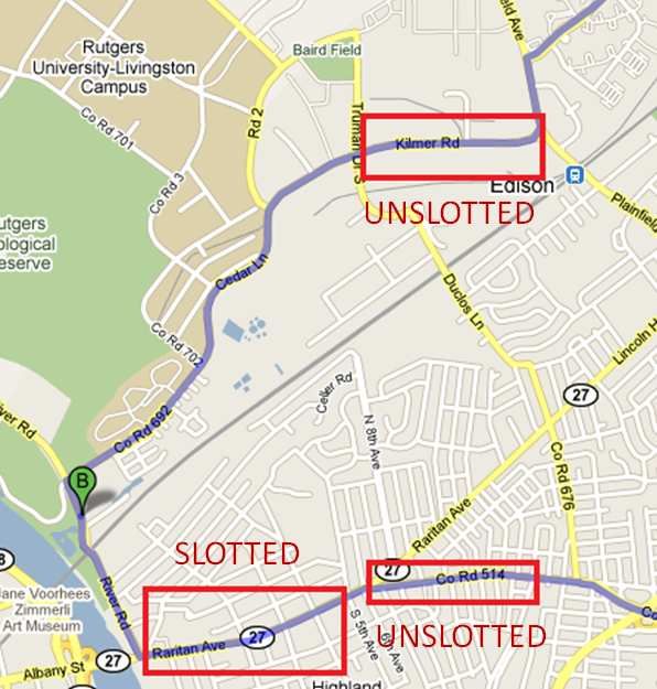
Figure 3: A diagram depicting the various scenarios and events involved in the detection of parking space
using mobile sensors.

approach is difficult because it (i) requires exact knowledge       • Improve efficiency of parking enforcement in systems
of the available road-side parking spots at any given time,           that utilize single pay stations for multiple parking
(ii) requires all other vehicles to be notified of and to obey        spaces – parking enforcement vehicles can detect the
reservations, (iii) may lead to inefficiencies if drivers with        presence of a parked vehicle in a space that has not
reservations do change their plans or experience significant          been paid for.
travel delays. While this approach presents interesting re-
search challenges, we chose to focus on a different approach        Parking information in slotted and unslotted ar-
that in our opinion has more potential for near-term im-         eas. To define concrete parking metrics it is helpful to dis-
pact: presenting drivers and municipal governments with          tinguish areas where vehicles are arranged in slots with de-
near-real-time information and detailed historical parking       marcated parking bays (often separated by lines marked on
statistics.                                                      the road), which we refer to as slotted areas, from areas
   Value of Real-time Information. As Donald Shoup               without any marked parking spots, which we will call unslot-
has argued [5] municipalities already posses parking man-        ted. Slotted parking space are typically used where parking
agement tools such as parking meters and pay stations and        meters or other parking pay stations are installed. This is
a large share of excess vehicle miles due to the search for      arguably the more important case, because parking is usu-
parking could be eliminated through basic road-side park-        ally slotted and metered in the areas where parking is most
ing price adjustments. Shoup concludes that prices should        scarce. In such areas it is easier to measure the number of
be set to achieve an 85% occupancy rate on each block. This      available parking spaces, because the spacing between cars
approach, however, would require detailed occupancy rate         is regulated. We consider two types of parking information:
information that allows parking authorities to adjust prices
and to determine which city areas should be included in the      Space Count. The number of parking spaces available on
pricing scheme.                                                      one given road segment, which is simply the total num-
   Beyond adjusting road-side parking prices, detailed park-         ber of marked parking spots less the occupied slots.
ing availability statistics could be widely disseminated on      Occupancy Map. A map showing each parking slot as oc-
web-based maps or navigation systems which would incur               cupied or vacant. This is more detailed representation
the following further benefits:                                      of the parking scenario which will be of particular in-
                                                                     terest in assisting parking enforcement.
   • Improve traveler decisions, with respect to mode of
     transportation, the choice of road-side parking vs park-       We expect that periodic per-block space counts are suffi-
     ing garage, and in which area to search for road-side       cient for many parking information applications. Occupancy
     parking,                                                    maps are immensely valuable for parking enforcement. A
                                                                 parking enforcement vehicle with a sensor and connectivity
   • Suggesting parking spaces to users driving on the road      to a database that keeps track of which slots have been paid
     looking for parking, through a navigation device or         for, would be able to determine whether there is a car parked
     cellphone,                                                  in a slot that has not been paid for, or whose time has ex-
                                                                 pired. This is particularly relevant for street-parking areas
   • Allow parking garages to adjust their prices dynami-        with a single payment machine for a large group of slotted
     cally to respond to the availability or non-availability    spaces, since the lack of parking meters for individual spaces
     of parking spaces in the immediate area, and                makes the task of finding offending vehicles harder.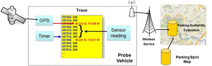
Figure 4: Schematic diagram explaining the overall architecture of the system.

   In the case of unslotted street parking, the number of                sor can do the work of hundreds of fixed sensors and if we
available slots is not defined a priori and depends on the               accept the limitations of a probabilistic system, costs can
length of vehicles. Still some parts of the road might be                be reduced further by mounting the mobile sensors on exist-
marked as no parking zones either explicitly or implicitly by            ing vehicles that roam the city, albeit perhaps on somewhat
the presence of driveways or fire hydrants for example. To               unpredictable paths.
define a space count for unslotted areas, we measure the dis-
tances d1 , d2 , . . . ...dn of all available stretches of valid park-   2.1 Design Goals and Requirements
ing (which are bounded by parked vehicles or no parking                    We identify the following design goals and requirements
zones) on a given road        P segment. The number of spots is          that constrain our solution:
then defined as n = i ⌊di /dspot ⌋, where dspot is taken to
be the (fixed) size of one parking spot (typically ∼ 6 me-               Provide Parking Statistics. The drive-by monitoring sys-
ters). The equivalent of the occupancy map for the unslot-                   tem should be able to determine the availability of
ted model will be the series of available parking stretches                  road-side parking spaces on at least an hourly basis
d1 , d2 , . . . , dn , together with the starting latitude/longitude         with sufficient accuracy to (i) direct drivers to areas
location stamp of each stretch.                                              with several available parking spots and to (ii) inform
   Indeed, some municipalities have already recognized the                   municipal government parking management decisions.
value of such detailed parking statistics and are installing
sensing technologies. The city of San Francisco, for example,            Assist Parking Enforcement. Given a map of paid-parking
is presently installing a stationary sensor network to cover                  spaces the drive-by sensing system should be able to
6000 parking spaces under the SFPark project [8]. This net-                   identify candidate parking spots occupied by an in-
work utilizes a sensor node installed in the asphalt in the                   fringing vehicle. Accuracy should be sufficient to as-
center of each parking spot. This node detects the pres-                      sign human parking enforcement personnel. The sys-
ence of a vehicle using a magnetometer among other sensors                    tem is not intended to generate automatic citations.
and forms a mesh network to deliver the data to a central-
ized parking monitoring system. To ensure connectivity, the              Low-cost sensors. The system should operate with sen-
mesh network also requires repeaters and forwarding nodes                    sors that are typically used in automobiles for other
on lamp posts and traffic lights.                                            applications. This rules out more expensive special-
   Installing a dedicated sensor network for monitoring park-                ized sensors such as laser scanners.
ing information is relatively expensive, due to the installa-
tion and maintenance costs. According to a Department of                 Low vehicle participation rates. While one could envi-
Transportation report [10], the installation cost of typical                 sion that eventually all vehicles simply report their
per spot parking management systems ranges from $250-                        parking locations as obtained from the Global Posi-
$800 per spot. While we do not know the exact cost of the                    tioning System, this would require the participation
system used by the SFPark project, the total project volume                  of nearly every vehicle to achieve high data accuracy.
including smart parking management functions is 23 million                   Given vehicle lifetimes of 10+ years in the United States,
dollars [8]. Furthermore, fixed sensors are quite difficult to               full deployment is difficult to achieve without govern-
place in areas without marked parking slots.                                 ment regulation mandating installation in every new
   What if it were possible to obtain most of the informa-                   vehicle or retrofitting of vehicles.
tion on the occupancy of parking spaces, at a much lower
cost? We believe sensing spaces using a collection of mobile             3. DRIVE-BY SENSING OF PARKING
sensors can provide such a solution because turnover on one
given parking spot is on the order of tens of minutes in the                AVAILABILITY
most expensive downtown areas and hours in many more                       The ParkNet architecture employs a mobile sensing ap-
residential city areas. Thus the required per-spot sampling              proach with ultrasonic rangefinders and GPS to monitor
rate is relatively low and the use of one dedicated sensor               road-side parking availability. It also introduces an envi-
per spot appears wasteful. Intuitively, a single mobile sen-             ronmental positioning concept to achieve the positioning ac-
                                                                         curacy necessary to match vehicles to demarcated parking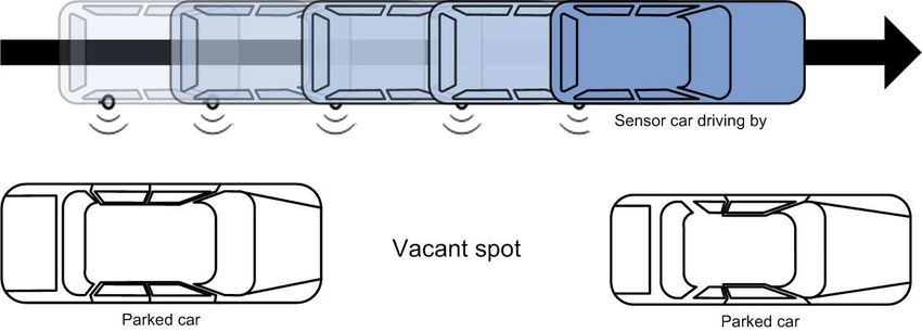
(a)                                  (b)                                (c)

Figure 5: (a) An image of the ultrasonic sensor side-mounted on a car (b) The java applet we used for
recording ground truth from images. (c) The map of the data collection area.

slots. As illustrated in Fig. 4, several sensors-equipped ve-     abilistic detection algorithms that we will describe in the
hicles report their sensor readings to centralized parking es-    following sections.
timation server. This server combines information from a
parking spot map, which may be available in different levels      3.2 System Specifications
of detail (as we will discuss in Sec. 4 with the sensor read-       The on-board PC has a 1GHz CPU with 512 MB RAM, 20
ings from one or multiple vehicles obtained on the same road      GB hard disk space, an Atheros 802.11 a/b/g mini PCI card,
segment to create an estimate of road-side parking availabil-     and 6 USB 2.0 ports. We used a Garmin 18-5Hz GPS with
ity. Vehicles can report their data over a cellular uplink but    12 channel receiver that provides 5 fresh GPS readings per
opportunistic use of Wifi connections is also possible de-        second, and a real-time WAAS correction of errors less than
pending on cost/delay tradeoffs. The parking availability         3 meters. Both the sensor and the GPS provide data in serial
information can then be distributed to navigation systems         format, which can be accessed via an USB serial port on a
or distributed over the Internet, similarly to the various dis-   computer. Note that while we use an off-the-shelf GPS unit,
tribution channels for road traffic congestion information.       in practice, there exists the opportunity to use built in GPS
3.1 Choice of Ultrasonic Sensors                                  units in vehicles, which are sometimes wired together with
                                                                  the vehicle’s odometry to allow for better location accuracy.
   We chose ultrasonic rangefinders because of their rela-
tively low cost of tens of dollars compared to laser rangefind-
ers and automotive radars, better nighttime operation com-
                                                                  3.3 Prototype Deployment
pared to cameras, and their increasing availability in cars to       We implemented and deployed this system on three vehi-
support parking assistance and automated parking functions        cles which collected parking data over a 2 month time frame
in modern vehicles. This potentially allows reusing already       during their daily commute. Specifically, data was collected
present sensors in future vehicles.                               in three road-side parking areas in Highland Park, New Jer-
   Each sensor vehicle in our set-up carries a passenger-side     sey as depicted in Figure 5(b). One of these areas contained
facing ultrasonic rangefinder to detect the presence or ab-       57 marked slotted parking spots. The two unslotted areas
sence of parked vehicles. It’s range should be equal to at        are 734 m and 616 m in length. During the experiment time
least half the width of urban roads and the sampling rate         frame, we collected a total of more than ∼ 500 miles of data
high enough to provide several samples over the length of         on streets with parking. All data collected was from roads
a car at maximum city speeds. Figure 5(a) depicts our             with single lanes (see Section 7 for a discussion on multi-lane
prototype incarnation using a Maxbotix WR1 waterproof             roads). The data collection was not controlled in any man-
rangefinder, magnet-mounted to the side of a vehicle. This        ner (e.g. speed, traffic conditions, obstacles, etc.) – all data
sensor emits sound waves every 50 ms at a frequency of 42         was collected while drivers went about their daily commutes
KHz. The sensor provides a single range reading from 12 to        at various times of the day, oblivious to the data collection
255 inches every cycle, which corresponds to the distance to      process.
the nearest obstacle or the maximum range of 255 if no ob-           To obtain ground truth information for system evaluation
stacle is detected. The sensor measurements at each vehicle       purposes and to be able to analyze erroneous readings, we
are time-stamped and location-stamped with inputs from a          integrated a Sony PS3 Eye webcam into the passenger-side
5Hz GPS receiver, producing the following sensor records:         sensor mount. To avoid angular and shift errors with respect
                                                                  to the sensor, we mounted the camera just above the sen-
                  sor and aligned its orientation to the sensor. A user space
                                                                  program captures about 20fps and tags each image with a
  Vehicles transmit a collection of these measurements to         kernel time stamp. This time stamp links images to the sen-
the parking estimation server where data from mobile sen-         sor records obtained at approximately the same time. We
sors is continuously aggregated and processed using prob-         then manually inspected each image and entered the ground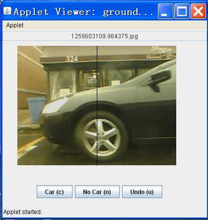
350
                                                                       350
     Sensor reading (inches)

                                             Sensor reading (inches)
                               300
                                                                       300
                               250
                                                                       250
                               200
                                                                       200
                               150
                                                                       150
                               100                                     100
                                50                                      50
                                 0                                       0
                               −50                                     −50

                                     (a)                                     (b)

Figure 6: Dips in the sensor reading as a sensing
vehicle drives past (a) two parked cars with some
space between them, and (b) two very closely spaced
parked cars

truth sensor data. For this process we implemented the java
applet depicted in Fig. 5(b). It displays each image together
with a reference line marking the estimated aiming of the
ultrasound sensor and allows the human evaluator to enter                          Figure 7: An example plot showing the sensor read-
whether the reference line crosses a parked vehicle. Note                          ing (dotted red) and ground truth (dashed blue line,
that the webcam is not part of the proposed parking sens-                          high = car, low = no car), speed (increased in mag-
ing system, it is purely used for evaluation and data analysis                     nitude by x10 for visual clarity), and the output of
purposes.                                                                          the detection algorithm (purple squares).

3.4 GPS trip-boxes for limiting data collection
   We limit data collection to the parking regions identified
in Fig. 5(c) due to the relatively small areas of roadside                         the distance to the nearest obstacle as the sensing vehicle
parking on one commute trip and the large volume of video                          moves forward. Figure 6 (a) shows an example of the trace
data involved. The activation and deactivation of data col-                        produced by our sensor as a sensing vehicle drives past two
lection is implemented in our system by using the idea of                          parked cars. We will refer to the features in Figure 6(a) as
a tripbox. Tripboxes are derived from our virtual trip line                        dips in the sensor reading. The width of a dip is represen-
concept [3], but represent rectangular areas defined by two                        tative of the length of a parked car, although, as we shall
(latitude,longitude) points. Each tripbox is also associate                        see, the errors in location estimates obtained from a GPS
with an entry and an exit function, which starts and stops                         receiver can distort the true length of the car in a somewhat
data collection, respectively. The tripbox daemon simply                           random manner. We assume that maps of areas with street-
reads the current GPS coordinates from the GPS receiver                            parking slots are available from another source (discussed
and checks whether it falls inside or outside the tripbox re-                      further in Section 7).
gion. If the current coordinate is the first instance of the
mobile node inside the tripbox, it triggers the entry func-                        4.1 Challenges
tion. In case the mobile node is already inside the tripbox                           An ultrasonic sensor does not have a perfectly narrow
and the next received coordinate is outside this region, it                        beam-width, but instead the beam width of the sound waves
triggers the exit function. We use tripboxes because it sim-                       emitted widens with distance. This implies that the sen-
plifies the handling of vehicle routes, which might enter a                        sor receives echos not just from objects that are directly in
parking zone from an unexpected direction, or the acquisi-                         front but also from objects that are at an angle. This af-
tion of a GPS fix while already inside a trip box.                                 fects how our sensor perceives vehicles that are parked very
   Since GPS coordinates can oscillate due to positioning er-                      close to each another. Instead of clearly sensing the gap be-
rors, the tripbox implementation includes a guard distance                         tween these vehicles, the ’dips’ in the sensor reading become
and a guard time to avoid repeatedly triggering the same                           merged, as depicted in Figure 6(b). Still, classification of the
tripbox functions. The guard distance is a minimum dis-                            spatial width of the dip allows us to determine the number
tance that must be traveled in between two tripbox bound-                          of cars that a dip corresponds to.
ary crossings. Similarly, the guard time is the minimum                               The inaccuracy of latitude and longitude values obtained
time that must be spent before the next tripbox function                           from the GPS unit adds another challenge to the detection
can be triggered. This avoids triggering the start and the                         problem. The location estimate provided by a commercial
stop functions repeatedly due to GPS errors.                                       grade GPS receiver suffers from well known errors. Without
                                                                                   a priori knowledge of how the GPS error varies in space and
                                                                                   time, it is possible that GPS errors can make a parked car
4.                             DETECTION OF PARKING SPACES                         appear to be shorter or longer than its true length. Since
  The detection algorithm translates the ultrasound distance-                      the detection of parked vehicles depends upon distinguish-
reading trace into a count of available parking spaces. The                        ing objects that are about the length of a car, from other,
distance-reading trace provides a one-dimensional view of                          smaller obstacles in the sensors path (such as trees, recycle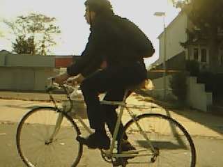
30

                                                                                             25

                                                                        Dip width (meters)
                                                                                             20

                                                                                             15

                                                                                             10

                                                                                              5

                                                                                              0
                                                                                                       50          100         150
                                                                                                  Distance from the sensor (inches)

Figure 8: A series of filters are applied to remove                Figure 9: A plot of the depth and width of most
dips in sensor readings that are not caused by parked              prominent dips observed in the sensor reading,
cars. We use 20% of our data to train our model and                caused by parked cars (blue squares) and objects
the remaining 80% to evaluate its performance.                     other than cars (red stars). This data set is taken
                                                                   from 19 trips in an area with slotted parking and is
                                                                   used for training the model used for classifying the
                                                                   rest of the data.
bins, people, etc.), this sometimes leads to false alarms (i.e.
dips caused by objects other than cars to be classified as
parked cars), and missed detections (i.e. parked vehicles to
be classified as something other than a parked car).               count the number of cars on a stretch of road. Subtracting
                                                                   this from the total number of slots on the road, as given
4.2 Detection algorithms                                           by the map, provides an estimate of the number of vacant
                                                                   spaces.
   Slotted model. Each dip in the sensor trace has depth              Unslotted model. For the unslotted parking model, the
and a width, that correspond to the distance from the sensor       number of cars that can be accommodated on a given stretch
of the object causing the dip, and the size of the object in the   of road depends upon the manner in which cars are parked
direction of motion of the sensing vehicle. The sensor trace       on it at any given instant of time. Since each successive pair
is first pre-processed to remove all dips that have too few        of parked cars in this model can have a variable amount of
readings (less than 6 sensor readings, assuming a maximum          space between them, we must estimate the space between
speed of 37 mph and a car length of 5 meters) and could            successive parked cars to determine whether the space is
not possible have arisen from a parked car. To detect a            large enough to accommodate one or more cars. To accom-
parked car, the width and depth of each dip in the sensor          plish this, we use the sensor trace to estimate the the spatial
reading is compared against thresholds. We determine these         distance between dips that have been classified as parked
thresholds using part of our data for training the system.         cars. The estimated length of the vacant stretch is then
Figure 8 shows a series of filtering stages that are applied       compared against the length of a standard parking space
to each detected dip in the sensor reading. Figure 9, shows        (which we have taken to be 6 meters).
the depth and width of the peaks observed in 19 separate
trips in an area with slotted parking. We used this data
for jointly picking thresholds for the depth and width of a
                                                                   4.3 Metrics
sensor-reading dip that provide the minimum overall error             We will deal with the slotted and unslotted street-parking
rate (i.e. the sum of the false positive rate and the miss         models separately and will assume that it is easy to obtain
detection rate1 ). These thresholds were determined to be          information about which streets have which type of parking
89.7 inches for the depth and 2.52 meters for the width,           as prior knowledge. For the slotted model, we are interested
resulting in an overall error rate of 12.4%.                       in detecting how many of the parking spaces on a road seg-
   Finally, all remaining dips are checked for spatial width,      ment are vacant.
and compared against a threshold representing the typical             Let us assume that a street segment with the slotted park-
length of a car. For this, we convert the interpolated GPS         ing model is known to have N parking slots and that at a
coordinates belonging to the starting and ending sample of         given instant of time, n of these slots are vacant. A sensing
the dip to UTM (meters) and compute the distance in meters         vehicle that drives through this street determines that n̂ of
between the starting and ending sample. Since some dips            the slots are vacant. The value of n̂ can differ from n due
correspond to multiple cars parked very close together, we         to missed detections as well as false positives. We are inter-
classify dips of a width greater than twice the threshold for      ested in the missed detection rate pm , i.e. the probability
one car, to belong to two cars, and so on. This allows us to       that a parked car is not detected, and the false positive rate
                                                                   pf , i.e. the probability that there is no parked car in a given
1
  The overall error rate is minimized when the false positive      slot but the detection algorithm detects one.
rate and the miss detection rate are equal in value [11].             The ratio n̂/n captures the performance of the detection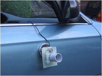
60
50 0.9
0.96 Mean ratio = 1.036
50
True # of cars parked
Detection Rate
0.94 40
True space (meters)
0.85
Detection rate
40
0.92 30
30 0.8
0.9
20
20
0.88 0.75
10 10
0.86 Mean ratio = 0.963
0.7
0.06 0.07 0.08 0.09 0.1 0 0
0 20 40 60 0 10 20 30 40 50 0.094 0.096 0.098 0.1
False Positive Rate Estimtated # of parked cars Estimated space between cars (meters)
False positive rate
(a) (b) (a) (b)
Figure 10: (a) Detection rate versus false positive Figure 11: (a) Scatter plot showing the estimate
rate for the slotted parking model. (b) A scatter of the space between cars Vs. the true space as ob-
plot showing the number of vehicles detected against tained from video measurements. (b) Detection rate
the actual number of vehicles parked for the slotted versus false positive rate for the unslotted parking
parking model. Each data point represents a sepa- model, assuming at least 6 meters for a car to park.
rate run
for both our training data-set and the evaluation data-set.
algorithm in estimating the number of vacant spaces. This Figure 7 shows an example of a typical trace of the sensor
ratio can be smaller or larger than 1, for a given run, depend- reading along with the ground truth. Also shown in the im-
ing on whether there are greater number of missed detections age are the speed of the car and the cars detected as output
or false positives. Since our thresholds for dip classification of our detection algorithm. Figure 10(a) shows the trade-
are chosen from our training data to minimize the overall off between detection rate and false positives for the slotted
error rate, and this is known to occur when the probability model, as the threshold for the width of a dip (i.e. corre-
of false alarm equals the missed detection probability [11], sponding to the length of a car) is varied. We found that
we expect that the ratio n̂/n to have a mean close to 1. a threshold of 2.5 meters provides the best tradeoff in the
For the unslotted model, the appropriate metric of interest minimum probability of error sense. Figure 10(b) shows the
is: ‘How many more cars can be accommodated on a given number of detected parked vehicles on a road with 57 park-
road segment, given the cars that are presently parked on ing slots, against the true number of parked cars. We found
it?’. As explained in Section 4.2, estimating this number that on average, the ratio of the estimated number of cars
requires estimation of the space between parked cars. As to the true number of cars is 1.036, indicating a fairly good
in the slotted parking model, we will assume that we have estimator of the availability of free spaces.
available to us, the locations of stretches where unslotted For the unslotted model, we compare our estimate of space
parking spaces are available and we will run our detection between two successive cars with the true value as computed
algorithm only over such stretches. Whenever the detection using the ground truth generated by our tagged video im-
algorithm ascertains that a space between two parked cars is ages. The plot in Figure 11(a) shows this comparison as a
large enough to accommodate another car, it records the es- scatterplot. The estimates space is on average 96% of the
timated space d. ˆ Suppose the actual space between the cars true space. Further, the estimated space is compared with
is d, then dˆ can be larger or smaller than d and as before, we the length of a typical parking slot (usually about 6 meters)
ˆ
will take the measure of accuracy to be d/d. Further, we are to determine whether an additional car can be accommo-
interested in the miss detection rate pm , i.e. the probability dated. The result of this detection leads to false positives
that our algorithm decides that there isn’t enough space for and missed opportunities, and the trade-off between the cor-
a single car, when there actually is, and the false positive responding false positive rate and missed detection rate is
rate pf , i.e. the probability that the detection algorithm shown in Figure 11(b), as the threshold for the width of
declares that one or more cars can be accommodated in a a dip is varied. Figure 12 shows two examples of cases, as
space between two parked cars, whereas in reality there is captured by our webcam, where the detection algorithm was
not enough space for a single car. In our evaluation, we will fooled into making false alarm decisions.
assume a vehicle of length 5 meters and at least half meter Given that our estimate for the number of cars parked in
on either side for parking, for a minimum of 6 meters to the slotted model and the amount of space between succes-
qualify for a parking space. sive cars are 1.036 times and 0.963 times the true number
of cars and the true space respectively, we can say that the
system is approximately 95% accurate in terms of obtaining
4.4 Evaluation parking counts. In the following section, we will address the
To evaluate our detection algorithm, we utilize the images problem of trying to assign detected cars to specific slots in
recorded by the webcam in our set-up. Since the camera the slotted model.
records images at a rate of 21 frames per second, it matches
the rate at which sensor readings are recorded fairly well.
Each image is manually labelled based on whether the cen-
ter of the image has a car in front or not. The time stamp
associated with each image allows us to interpolate a loca-
tion stamp for each image. This provides the ground truth
1
                                                                                                                                               X (longitude)
                                                                                                           0.9                                 Y (latitude)

                                                                                                           0.8

                                                                                 Correlation coefficient
                                                                                                           0.7

                                                                                                           0.6

                                                                                                           0.5

                                                                                                           0.4

                                                                                                           0.3
                            (a)                           (b)
                                                                                                           0.2

                                                                                                           0.1
                                                                                                                 0   200     400      600       800        1000
Figure 12: (a) A moving bicyclist, and (b) a flower-                                                                       Distance (meters)
pot, both objects that produced dips in the sensor
trace that were classified incorrectly as parked cars                   Figure 14: Correlation in the error (with respect to
                                                                        centroid) of the GPS location estimates correspond-
                                                                        ing to fixed points along a road, as a function of
                                                                        distance along the road.
              3380

              3360                                                      receiver is affected by several factors including ionospheric
              3340                                                      effects, satellite orbit shifts, clock errors, and multipath.
                                                                        Ionospheric effect typically dominate the other error sources,
              3320
                                                                        except for errors that experience satellite occlusion (e.g., in
 Y (meters)

              3300                                                      urban canyons). Ionospheric effects remain similar over dis-
                                                                        tances of several 10s of kilometers and they contain signif-
              3280
                                                                        icant components whose rate of change is on the order of
              3260                                                      ∼10s of minutes or longer. GPS errors can therefore be ex-
              3240                                                      pected to be correlated in time and space. However, the
                                                                        Wide Area Augmentation System was designed to reduce
              3220
                                                                        these ionospheric and some other errors, raising the question
              3200                                                      whether the resulting GPS errors with WAAS still exhibit
                                                                        strong spatio-temporal correlation.
              3180
                     8000   8100   8200    8300    8400   8500   8600      We find that the GPS error is in fact highly correlated at
                                          X (meters)                    short distances, and the correlation tapers off with distance.
                                                                        Motivated by this observation, we propose a method to im-
                                                                        prove absolute location precision by an environmental fin-
Figure 13: The locations of 8 objects along a road                      gerprinting approach. In particular, we use the sensor read-
shown for 29 different runs.                                            ing to detect certain fixed objects that persistently appear
                                                                        in our ultrasound sensor traces, and utilize these to correct
                                                                        the error in the GPS trace. To validate the approach, we
5.             OCCUPANCY MAP CREATION WITH                              test it on the slot-matching problem described above. We
                                                                        expect that our environmental fingerprinting approach will
               ENVIRONMENTAL POSITIONING                                benefit any mobile sensing application that requires precise
               CORRECTION                                               estimates of location or distance between two points, as is
   While counting of available parking spaces did not re-               the case in some of the scenarios in our sensing application.
quire high absolute position accuracy, creating an occupancy
map of parking increases accuracy requirements since a de-              5.1 GPS Error Correlation
tected car has to be matched to a spot on a reference map.                 We began our study by location-tagging certain fixed ob-
The location coordinates provided by a GPS receiver are                 jects (such as trees, recycle bins, the edges of street signs,
only typically accurate to 3m (standard deviation) when the             etc. which would also be picked up by our sensor) in our
Wide Area Augmentation System (WAAS) service is avail-                  video traces on a given street over multiple different runs
able [12, 13]. Given a parking spot length of about 7m, one             from different days. We tagged the data with the same video
can expect a significant rate of errors—any error greater               tagging application we developed for evaluating our detec-
than 3.5m could lead to matching a vehicle to an incorrect              tion algorithm (see Figure 5(c)). We found, as expected that
adjacent spot.                                                          the tagged coordinates for a given object from multiple runs
   To address the occupancy map challenge, we develop a                 varied significantly. Using 29 different runs and 8 objects
occupancy map creation algorithm that exploits both pat-                on a street, we found the standard deviation of error to be
terns in the sequence of parking spots as well as an Envi-              4.6 m in the X-direction and 5.2 meters in the Y-direction.
ronmental GPS position correction method to improve lo-                 We note here that the error due to variation in the lateral
cation accuracy with respect to the parking spot map. We                position of the sensing vehicle was not corrected for because
first study how the error in GPS coordinates behaves as a               the street chosen for this was narrow enough to allow the
function of distance. The positioning accuracy of a GPS                 lateral variation to be within ±1/2 meter. Also this street
1 20 20 20 25
Uncorrected data
19.6% With fingerprinting
0 0 0 0 20
Percentage errors
−1 −20 −20 −20 15 13.5%
−1 0 1 −20 0 20 −20 0 20 −20 0 20
20 20 20 20
10 8.8%
6.1%
0 0 0 0 4.5% 4.3%
5
−20 −20 −20 −20
−20 0 20 −20 0 20 −20 0 20 −20 0 20 0
Overall False positives Miss detections
Figure 15: Using the first object in a series of 8
objects to correct the error of the remaining 7 ob- Figure 16: A comparison of the error rates in assign-
jects. The plots are arranged in increasing order of ing parked cars to the correct slots with and without
distance from object 1, from left to right and top to error correction using fingerprinting.
bottom. The colors match those of objects in Figure
13 (axes are in m). Location error builds up with
increasing distance from the object 1. consists of dips within a radius of 20 meters of the known
mean location of the fixed object (mean computed from past
traces). We then select one dip from each candidate set so
was almost parallel to the X axis and so we expected to ob- that the distance between the successive selected dips best
serve an larger error in the Y direction to slight variaions in matches the known distance between the mean locations of
the sensing vehicle’s lateral position. the objects to which they correspond. The vector offset be-
We also found that the error between GPS coordinates tween the known locations and the reported locations of the
is correlated from one object to the next. Figure 13 shows objects is the GPS error estimate. The correction procedure
the locations of the 8 objects along the street. We chose must be repeated with another set of objects once the vehicle
the centroid of the 29 tagged locations for each object as travel distance has exceeded the correlation distance.
the reference location and subtracted each tagged location For n such objects, i = 1, . . . n, we recorded the loca-
coordinate to compute the error. Figure 14 shows the cor- tion stamps li (x, y) of the dips corresponding to each object
relation between the error in the X and Y directions as a and subtracted it from the known true location of the ob-
function of distance along the street, using the 8 objects we ject ti (x, y) (assuming the centroid of the 29 locations as
selected. It is worth noting that the correlation in the error above), giving an estimate of the error vector ei (x, y) =
is fairly high for a distance of up to ∼ 250 meters. ti (x, y) − li (x, y). Next, this error vector from a given object
is added to the location estimates of all detected cars that
5.2 Environmental Fingerprinting are detected to be within 100 meters of this object.
The above investigation suggests that if the GPS error is
corrected at a given point, then it is likely to remain cor- 5.3 Slot-matching
rected for an appreciable distance. In Figure 15, we utilize Motivated by our observation of correlation between GPS
the location-stamp of the first object on the street (lower error in space, we studied the specific application of match-
left corner in Figure 13) to correct the errors in the loca- ing detected parked cars to their respective slots on a street
tion of the remaining 7 objects. As Figure 15 illustrates, the with slotted parking. To accomplish this, the output of the
residual error in the error-corrected location-stamp for the algorithm for detecting cars in the slotted model (see Fig-
7 objects increases with increasing distance from object 1. ure 8) was augmented with the estimated location of each
Fingerprinting the environment by relying on features in detected car. The locations of 57 slots on a street were de-
the sensor trace that are produced by fixed objects in the termined using a satellite picture from Google Earth. The
environment, provides a possible means to improve location matching of cars to slots is an instance of the assignment
accuracy beyond that provided by GPS alone. However, fin- problem [14] on bipartite graphs and can be solved efficiently
gerprinting a street requires multiple traces from that street, using the Hungarian algorithm [15]. The problem involves
from which the locations of objects that are very likely fixed assigning each detected parked car with specified location
can be determined. coordinates in the set of detected cars, to a valid slot from
Estimating the GPS error using the sensor trace involves among the set of 57 slots available. The criterion for the
a simple task — comparing the reported location of the pat- assignment is the minimization of the cumulative distance
tern (dips) produced by a series of fixed objects to the a between each car and its assigned slot. We used a MATLAB
priori known location of this pattern (as determined from implementation of the Hungarian algorithm to solve for the
multiple previous traces from the same road segment). The slot-matching of detected parked cars.
offset between the two gives an estimate of the error in the Figure 16 shows the error-performance of the slot-matching
reported location. algorithm, when using plain uncorrected traces and with
For example, to detect the dips corresponding to two suc- traces that have been corrected using the fingerprinting al-
cessive fixed objects from an experimental trace, we first gorithm described above. We find that the fingerprinting ap-
identify a set of candidate dips for each object from the proach described in the previous section segnificantly lowers
dips that are not classified as vehicles — each candidate set the error rate in slot assignments.(a) (b) Figure 17: (a) Two areas of San Francisco (one larger and the other, a smaller downtown area) in which we monitored the movements of 536 taxicabs over a stretch of one month (b) Location trace of a single taxicab in San Francisco area over a span of 30 days. The areas with highest presence are also the busiest areas with most street-parking. 6. MOBILITY STUDY that all present pilot installations of fixed parking sensors The viability of ParkNet and its desirability over static under the SFpark project are in the smaller area in Figure sensor systems that monitor parking is intimately tied to the 17(a) (see [8] for a map) and that the taxicab trace also number of mobile sensors that must be deployed in order to reveals that cabs spend most time in this area (see Figure adequately monitor street-parking spaces. In particular, it 17(b)). is important to determine how often, statistically speaking, We divided each area into a grid of cells that were 175×190 a ParkNet mobile node would pass by on a randomly picked meters in size, and computed for each cell, the mean time street, and how this quantity varies as the number of mobile between successive visits by a taxicab in the fleet. We chose nodes in ParkNet is varied. This relationship could them the size of a cell so that is most cases, only a single road be used to determine whether the underlying tradeoff allows segment is contained within a cell. Our findings are summa- for significantly fewer (mobile) sensors to be employed in rized in Figure 18(a) for the larger area and in Figure 18(b) ParkNet than a system with stationary sensors, and if so, for the smaller, busier area. We find, even with roughly 500 what level of cost savings can be expected. cabs deployed in the greater San Francisco area, the mean In order to realistically explore this question, we con- time between visits to a cell is on the order of hundreds of ducted a study of the mobility patterns of taxicabs using a minutes. On the other hand, the sampling provided by these public dataset of 536 taxicabs in San Francisco collected over same cabs in the smaller, downtown area of San Francisco a span of roughly one month during 2008 [16]. The dataset more than adequately covers the smaller area, with 80% of contains time-stamped location traces for each taxicab with the cells visited on average with an inter-visit interval of successive location updates being recorded 60 seconds apart. under 10 minutes with just 536 cabs. Using this trace as Figure 17(b) shows the locations of a single taxicab in this a guideline for other urban areas, one can extrapolate to data-set over a span of 30 days. We approximated the inter- estimate the number of taxicabs that must be fitted with a mediate locations of each taxicab by linearly interpolating sensor in order to provide a sufficiently small inter-visit time locations between successive GPS updates. between successive visits to a randomly chosen street. We considered two geographical areas, shown in Figure Cost analysis: A rough analysis of our system reveals 17(a): (i) the greater San Francisco area, and (ii) the busi- that the basic components in our system cost approximately est portion of San Francisco where the business districts and ∼ $400 for one sensing vehicle (a light-weight PC platform: tourist attractions are concentrated. The latter is also hap- $170, sensor: $20, GPS unit: $100, and $100 for wiring and pens to contain all the installations of the SFpark project [8]. connecting components including labor). In comparison, [10] We conjecture that areas with a greater amount of street estimates a cost of $250-$800 per space for a ‘smart park- parking utilization are also the areas with a greatest pres- ing system’. Even taking a conservative estimate of $250 ence of taxicabs since both are driven by large concentrations per spot, a system consisting of fixed sensors, covering 6000 of people. This hypothesis is supported by the observation parking spaces in the upper left corner of San Francisco (as
1                                                          1
                                                  50 cabs
                                                  100 cabs
                                    0.8           200 cabs                                     0.8

                    Empirical CDF
                                                  300 cabs

                                                                               Empirical CDF
                                                  536 cabs
                                    0.6                                                        0.6

                                    0.4                                                        0.4
                                                                                                                           50 cabs
                                                                                                                           100 cabs
                                    0.2                                                        0.2                         200 cabs
                                                                                                                           300 cabs
                                                                                                                           536 cabs
                                          0        50        100   150   200                    0
                                                                                                 0        50     100     150      200
                                              Mean time between cabs (min)                           Mean time between cabs (min)
                                                             (a)                                                (b)

Figure 18: The cumulative distribution function of the mean time between successive taxicabs visiting a
street in (a) greater San Francisco (b) smaller, busier downtown area, as the number of cabs being considered
part of ParkNet is varied. To compute the CDF, the city is divided into cell of size 175 m × 190 m

a pilot, the SFpark project has installed 6000 sensors in this                    25 minutes would necessitate that our system be deployed
area of San Francisco at the time of this writing), this would                    in roughly 2000 cabs). Even so, the cost benefits associated
incur a cost of $1.5M for the fixed sensor system. On the                         with ParkNet are still significant as it is not necessary to
other hand, with only 300 cabs (see Figure 18(b)), which                          have continual sampling of parking space occupancy.
provide an average inter-polling time of ∼ 25 minutes for
80% of the cells, the corresponding cost is roughly $120,000,
giving a equipment cost saving factor of 12.5. Note that                          7. DISCUSSION AND LESSONS LEARNED
this number represents a conservative estimate of the cost                           Apart from the challenges faced while meeting real-time
savings, since (i) in practice, the cost of the mobile sens-                      localization of vacant parking spots, the gathering and pro-
ing system per mobile node can be brought down below our                          cessing of reliable sensor data poses its own set of difficulties.
estimate of $400 with aggressive engineering and mass pro-                        We discuss the details of the most challenging issues we en-
duction, and (ii) we have chosen the lower end of the cost                        countered below.
estimate per spot for the fixed sensor system. Note fur-                             Power source. One unexpected difficulty turned out to
ther, that San Francisco city is estimated to have 281, 364                       be noisy sensor data affected by the power source for the
road-side parking spaces, of which 24, 464 are estimated to                       in-car nodes. Initially, we used a power inverter to convert
be metered spaces [17]. While only 6000 spots considered                          the 12 volt DC vehicle power supply to AC power suitable
‘high-value’ spots by the city of San Francisco have been                         for a standard PC power supply. Although this setup sup-
fitted with fixed sensors, we do not know how many of the                         plied adequate power, it lead to very noisy sensor data. The
total 24, 464 metered spots are within the downtown area we                       ultrasound transducer may have been affected by the mod-
have considered. The cost saving factor is therefore likely                       ified sine wave output of the inverter, which is known to
to be larger when the actual number of spots in this area is                      affect sensitive electronic equipment. To address this is-
considered.                                                                       sue, we installed DC to DC power supplies in each car node
   The operational running cost of each system comprises                          and connected them directly to the fuse box. This solution
maintenance and communications costs. We expect the to-                           worked in some vehicles, but in vehicles with weaker battery,
tal operational cost of ParkNet to be less than that of a                         turn-on of the vehicle node was unreliable.
fixed sensor system. Communications in ParkNet can be                                Multilane roads. Detecting parked cars on a multi-lane
done over opportunistic WiFi connections in urban environ-                        road requires lane-detection so that vehicles being passed or
ments, making it almost free, and maintenance is expected                         passing the sensing car in a different lane are not classified
to be more easily manageable than a fixed system because                          as parked cars. GPS accuracy is unlikely to be sufficient for
the number of mobile nodes is much smaller than the num-                          lane detection. The data collected and reported upon in the
ber of fixed sensors, and taxicabs are regularly taken in for                     paper was taken entirely on single-lane roads. We found,
maintenance into garages.                                                         however, through preliminary trials that it is often possible
   We note however, that the cost benefit that mobile sens-                       to distinguish moving vehicles in the neighboring lane from
ing provides comes from the fact that it provides a non-                          parked vehicles by the length of sensor dips. A car moving
guaranteed, random sampling of the parking process, whereas                       at similar speeds as the sensing vehicle, for example, will
fixed sensor provide continuous monitoring wherever they                          generate a very long dip. Another promising approach is to
are installed. Hence, the cost associated with our system                         use a sensor with a much larger range – this can greatly help
does increase as we require that a higher fraction of cells be                    lane detection.
covered (for e.g. extrapolation shows that requiring 95% of                          Speed limitations. A limitation of using an ultrasonic
the cells be sampled with a mean inter-sampling period of                         sensor is that we are limited by the speed of sound. Our
                                                                                  sensor provides a maximum range of 6.45 meters, and since
it must wait for a return echo before sending out the next at fairly high cost of operation and only for metered spaces
pulse, the sensor provide only 20 distance readings per sec- and garages. In contrast, the mobile sensing approach pro-
ond. This implies that if the sensing vehicle is driving too posed in this paper provides a probabilistic alternative at a
fast, it will not be able to sense a parked vehicle. For ex- potentially much lower cost, and can work for both metered
ample, at a speed of 15 meters per second (roughly 33 miles slotted spaces as well as unslotted spaces.
per hour), a 5 meter long parked car should produce about Another line of work related to ours is the estimation of
∼ 6 distance readings from the sensor. However, the speed traffic conditions on roadways using mobile sensing. The au-
limit in areas with street parking is usually in the range of thors in [2] propose techniques to mine location trace data
35– 40 miles per hour and so our choice of sensor should not reported by vehicles on streets reporting their locations in-
be a limiting problem. frequently over a cellular uplink, to characterize traffic pat-
Obtaining parking spot maps. One issue that may terns on road segments. VTrack [25] explores the use of com-
seem to limit large deployments is the effort to obtain park- modity smartphones for localization using cellular and WiFi
ing spot maps, particularly when complicated time-dependent signals in addition to GPS for localization to estimate traf-
parking rules are in place. Beyond manual construction from fic delays on roadways with fine spatio-temporal granularity.
satellite imagery, as in our project, maps may be available to Their work focuses on the challenges associated with energy
some extend at city authorities. We believe, however, that consumption and the unreliability of sensors. Nericell [26]
maps can also be automatically generated through aggrega- also utilizes sensors available on smartphones to detect road
tion of sensor data over time periods of weeks to months. and traffic conditions in a city, using microphones to detect
The intuition behind this idea is simple: spaces that al- the level of honking and accelerometers to detect bumps and
most never have cars parked are likely to be invalid parking braking. Other work in mobile sensing includes [9] which
spaces (driveways, storefronts, illegal parking spots such as uses the mobility of participating vehicles to detect potholes
fire-hydrants, etc., or simply portions where parking is not in roads using accelerometers, and aggregate this data over
allowed), while spaces that always have a car parked are very time to obtain the locations of the roads that are most in
likely not parked cars, but some other immovable object. need of repair. [3] uses the concept of virtual triplines to
address the privacy problems in traffic monitoring systems
8. RELATED WORK based on the reporting of GPS coordinates by individual
users.
A number of approaches have been tested for the moni-
Prior work on getting location information in mobile sys-
toring of parking spaces in recent times. Parking garages
tems has focussed heavily on the use of GPS receivers. Re-
have been using in/out counters at the entry and exit points
cent research on localization has also explored the use of
to count the number of additional vehicles they can accom-
GSM cellular signals for triangulation of cellphones [27]. Al-
modate at any given time [18]. This information is often
though cellular signals provide much lower location preci-
displayed on prominent electronic signs-boards near such
sion, they have also been used for traffic monitoring appli-
garages or on nearby roadways, allowing drivers to decide
cations [25, 28, 29]. Finally, our work on improving location
which way to go to find parking. Airports and rail stations
accuracy using the sensor in addition to the GPS, may be
have been using similar parking management systems in re-
thought of as a locationing system with the fusion of infor-
cent times [18]. A somewhat newer approach to finding and
mation from multiple sensors, on which there exists exten-
reserving parking spaces in urban areas, albeit with very
sive past literature (see for e.g. the location stack [30, 31]
limited success, has been tested by web-based markets such
built by Hightower and Fox).
as those in [19, 20] that allow users to buy and sell parking
spaces on the internet for specified times. Such an inter-
net marketplace allows for owners of private spots (such as 9. CONCLUSIONS
residential spaces) and parking garages to offer reservations We have presented the ParkNet system, a mobile approach
to users looking for parking, and for people occupying pub- to collecting road-side parking availability information, which
lic metered spaces to broadcast the time at which they will introduced more challenging location accuracy and sampling
be vacating the parking spot. Needless to say, no reserva- frequency requirements than earlier vehicular sensing appli-
tion mechanism is possible for metered public spaces. Other cations. Based on over 500 miles of data collected over 2
web-based systems such as [21,22] allows travellers to access months with our prototype vehicles, we showed that ultra-
information about the availability of spaces at airports or sound sensors combined with GPS can achieve about 95%
rail stations and make prior reservations. In the academic accurate parking space counts and can generate over 90%
literature, [23] demonstrated a toy system that monitors accurate parking occupancy maps. To create occupancy
individual parking spaces using web cameras, allows users maps, we corrected GPS errors using environmental refer-
to query the system for vacant spaces on a web front-end ences points, since we found that GPS error were correlated
and provides the user with the closest vacant parking space over time and space even with WAAS support. Using trace-
that meets the constraints entered by the user. Metered driven simulations from San Francisco taxicabs we showed
parking in the city of Chicago recently went through major that equipping only 536 vehicles with sensors would lead to
changes [24] – individual parking meters were replaced with a mean inter-sampling interval of about 25min in 85% of the
pay stations that handle a large number of parking spaces. downtown area, or about 10 min in 80% of the area. Fur-
Doing away with individual parking meters makes the detec- ther, we expect that the density of taxicabs in an urban area
tion of offending vehicles parked in unpaid spots by parking to be strongly correlated with the presence of street parking
enforcement authorities harder. Using the slot-matching ap- spaces, since both are driven by the presence of a large num-
proach described in this paper, such detection can be greatly ber of people. With the small number of sensors required,
simplified. SFPark [8] is the only system in our knowledge the mobile sensing approach therefore promises significant
that specifically monitors street-side parking spaces, albeit, cost benefits over current stationary sensing approaches—You can also read