On-sky results for the novel integrated micro-lens ring tip-tilt sensor
←
→
Page content transcription
If your browser does not render page correctly, please read the page content below
Research Article                                                                                           Journal of the Optical Society of America B   1

                                               On-sky results for the novel integrated micro-lens ring
                                               tip-tilt sensor
                                               P HILIPP H OTTINGER1,* , R OBERT J. H ARRIS1,2 , J ONATHAN C RASS3 , P HILIPP -I MMANUEL D IETRICH4,5,6 ,
                                               M ATTHIAS B LAICHER4,5 , A NDREW B ECHTER3 , B RIAN S ANDS3 , T IM J. M ORRIS7 , A LASTAIR G.
                                               BASDEN7 , N AZIM A LI B HARMAL7 , J OCHEN H EIDT1 , T HEODOROS A NAGNOS1,2 , P HILIP L.
arXiv:2106.10152v1 [astro-ph.IM] 18 Jun 2021

                                               N EUREUTHER8 , M ARTIN G LÜCK8 , J ENNIFER P OWER9 , J ÖRG -U WE P OTT2 , C HRISTIAN KOOS4,5,6 ,
                                               O LIVER S AWODNY8 , AND A NDREAS Q UIRRENBACH1
                                               1 Landessternwarte,    Zentrum für Astronomie der Universität Heidelberg, Königstuhl 12, 69117 Heidelberg, Germany
                                               2 Max-Planck-Institute   for Astronomy, Königstuhl 17, 69117, Heidelberg, Germany
                                               3 Department of Physics, University of Notre Dame, 225 Nieuwland Science Hall, Notre Dame, IN 46556, USA
                                               4 Institute of Microstructure Technology (IMT), Karlsruhe Institute of Technology (KIT), Hermann-von-Helmholtz-Platz 1, 76344 Eggenstein-Leopoldshafen,

                                               Germany
                                               5 Institute of Photonics and Quantum Electronics (IPQ), Karlsruhe Institute of Technology (KIT), Engesserstr. 5, 76131 Karlsruhe, Germany
                                               6 Vanguard Photonics GmbH, Hermann-von-Helmholtz-Platz 1, 76344 Eggenstein-Leopoldshafen, Germany
                                               7 Department of Physics, Durham University, South Road, Durham, DH1 3LE, UK
                                               8 Institute for System Dynamics, University of Stuttgart, Waldburgstr. 19, 70563 Stuttgart, Germany
                                               9 Large Binocular Telescope Observatory, 933 N. Cherry Ave, Tucson, AZ 85721-0009, U.S.A.
                                               * phottinger@lsw.uni-heidelberg.de

                                                © 2021 Optical Society of America]. One print or electronic copy may be made for personal use only. Systematic reproduction and distribution, duplication of
                                               any material in this paper for a fee or for commercial purposes, or modifications of the content of this paper are prohibited.

                                               Compiled June 21, 2021

                                                      We present the first on-sky results of the micro-lens ring tip-tilt (MLR-TT) sensor. This sensor utilizes
                                                      a 3D printed micro-lens ring feeding six multi-mode fibers to sense misaligned light, allowing centroid
                                                      reconstruction. A tip-tilt mirror allows the beam to be corrected, increasing the amount of light coupled
                                                      into a centrally positioned single-mode (science) fiber. The sensor was tested with the iLocater acquisition
                                                      camera at the Large Binocular Telescope in November 2019. The limit on the maximum achieved root
                                                      mean square reconstruction accuracy was found to be 0.19 λ/D in both tip and tilt, of which approximately
                                                      50% of the power originates at frequencies below 10 Hz. We show the reconstruction accuracy is highly
                                                      dependent on the estimated Strehl ratio and simulations support the assumption that residual adaptive
                                                      optics aberrations are the main limit to the reconstruction accuracy. We conclude that this sensor is ideally
                                                      suited to remove post-adaptive optics non-common path tip tilt residuals. We discuss the next steps for
                                                      the concept development, including optimizations of the lens and fiber, tuning of the correction algorithm
                                                      and selection of optimal science cases. © 2021 Optical Society of America
                                                      http://dx.doi.org/10.1364/ao.XX.XXXXXX

                                               1. INTRODUCTION                                                                   of correction provided by these ExAO systems also makes it pos-
                                                                                                                                 sible to efficiently couple light from the telescope directly into
                                               In recent decades, improvements in the performance of an in-                      single-mode fibers (SMFs) [6]. SMFs have a core diameter of the
                                               creasing number of extreme adaptive optics (ExAO) systems has                     order of ten microns, which can only transport the fundamental
                                               led to the ability to image near the diffraction-limit using 8 m-                 fiber mode. As this mode is the only spatial mode transported
                                               class telescopes [1–4]. These ExAO systems focus on achieving                     and has a near-Gaussian intensity profile, the corresponding out-
                                               the best performance over a small field of view (FoV) and regu-                   put beam is very stable and easy to model. SMFs also act as a spa-
                                               larly achieve Strehl ratios (SRs) of 80% in the near-infrared (NIR).              tial filter and couple very little sky background [7]. This makes
                                               One of the most prominent goals for these systems is the direct                   them highly suitable for direct exoplanet spectroscopy [8] and
                                               observation and characterization of exoplanets [5], for which                     interferometry [9–13]. When coupled to a high resolution spec-
                                               high angular resolution and contrast are crucial. The high level                  trograph, SMFs also remove conventional modal noise, allowing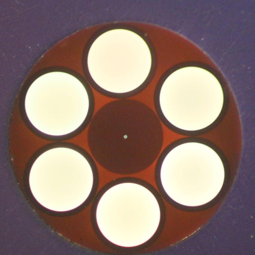
Research Article                                                                      Journal of the Optical Society of America B   2

 an increase in the achievable radial velocity (RV) precision [14].      systems utilizing concurrent alignment lasers [25]. While most
 A number of SMF-fed spectrographs are currently under devel-            of these systems have been adopted at large telescopes, they all
 opment, including iLocater at Large Binocular Telescope (LBT)           have a significant mechanical and optical footprint, throughput
 [7, 15], SPHERE and CRIRES+ at the Very Large Telescope (VLT)           loss, tend to become complex in operation, and are vulnerable
 [16], RHEA and IRD at SCExAO/Subaru [17, 18] and KPIC at                to non-common path (NCP) effects as the tip-tilt correction is
 Keck [19].                                                              performed at a different optical surface than the SMF face.
     As the size of the fiber is of the order of the diffraction limit       Different fiber based photonic sensor concepts are being in-
 (λ/D, where λ is the wavelength and D the diameter of the               vestigated in the community to complement conventional AO
 telescope), the alignment accuracy is highly dependent on the           systems [26, 27]. The concept presented in this work draws from
 point-spread function (PSF) stability (see Fig. 1 for an example        Ref. 28, who developed a sensor with multiple single-mode (SM)
 of relative coupling efficiency as a function of residual tip-tilt      cores equipped with an micro-lens array to refract the beam at
 position). Any vibrations that occur throughout the telescope           the focal plane for both science instrument and tip-tilt sensing.
 system and influence the position of the PSF in the focal plane         Our modified concept features multi-mode fibers (MMFs) in
 can have a large impact on performance. These variations can            conjunction with a micro-lens ring (MLR) [29] for sensing and
 be caused by electrical and mechanical components such as fans          is called the micro-lens ring tip-tilt (MLR-TT) sensor [30]. We
 and pumps, but can also be induced by wind, atmospheric dis-            present first on-sky results of this novel tip-tilt sensor with the
 tortions and dome seeing [20]. As these variations can have both        iLocater acquisition camera at the LBT [15].
 large amplitude and high frequencies, the adaptive optics (AO)              In Section 2, we describe the sensor concept and the methods
 system may not be able to compensate for them sufficiently and,         used to design, manufacture and employ it at the telescope
 if they can occur outside the path to the wavefront sensor (WFS),       along with outlining our simulation approach. In Section 3
 they will not be sensed. These variations can effect the perfor-        we present our on-sky results and supporting simulations and
 mance significantly [21] and turn out to be a limiting factor when      in Section 4 we discuss these results and future developments
 coupling into SMFs, with coupling efficiency being degraded by          before presenting our conclusions in Section 5.
 as much as a factor of two [22].
                                                                         2. DESIGN AND METHODS
                                                                         The MLR-TT sensor concept is depicted in Fig. 2 as both a
                                                                         schematic cross-section of the optics (Fig. 2, left-hand side) and
                          1.00                             Model         as images of the manufactured components (Fig. 2, right-hand
SMF coupling efficiency

                                                                         side). The details are re-iterated here, with additional informa-
                                                           iLocater
                                                                         tion, for clarity:
                          0.75                             iLocater
                                                           + quad-cell    1. The sensor consists of a fiber bundle containing six MMFs
                                                                             surrounding an SMF, located at the iLocater focal plane. On
                          0.50                                               the fiber face, an MLR stands 380 µm tall and 355 µm wide
                                                                             with a central aperture of 86 µm.

                          0.25                                            2. The central part of the beam is injected into the SMF, while
                                                                             the outer edge is clipped and refracted by the MLR. De-
                                                                             pending on the alignment of the beam, the proportion of
                          0.00                                               light clipped by the MLR changes, which modifies the cou-
                                                                             pling into the individual MMFs.
                                 0.0          0.5           1.0
                                                                          3. The MMFs are separated from the SMF, re-arranged to form
                                       RMS tip-tilt combined [λ/D]           a linear array, re-imaged, and read out by a detector.
 Fig. 1. Numerically calculated theoretical normalized cou-               4. The illumination pattern of the MMFs is processed to recon-
 pling efficiency assuming an optimally coupled diffraction-                 struct the original PSF centroid position, which can be fed
 limited PSF with additional residual tip-tilt variation, plotted            back to a fast steering tip-tilt mirror for correction.
 in units of λ/D. The measured RMS residuals at the iLocater
 focal plane are also indicated, without beam stabilization at           A. Fiber bundle design
 0.61 λ/D resulting in a theoretical reduction by 44% (red line),
                                                                         The fiber bundle was manufactured commercially (Berlin Fibre
 and with additional stabilization with a quad-cell detector
                                                                         GmbH) and holds the array of seven fibers terminated into an
 improving tip-tilt stability to 0.39 λ/D, leading to a tip-tilt in-
                                                                         FC/PC connector which is then connected to the iLocater fiber
 duced coupling loss of 24% (green line) [15].
                                                                         feed mount. The fibers are stripped of their furcation tubing and
                                                                         buffer and are placed in the connector with a pitch of 125 µm.
    Besides high-order AO correction, efficient SMF-coupling             After 30 cm, the SMF and the MMFs separate into two individual
 therefore requires a method to accurately sense and correct in-         5 m-long fiber cables: 1) the science SMF, which is terminated
 duced tip-tilt variations. Traditionally, this is accomplished by       to an FC/PC adapter to feed the science instrument and 2) the
 detecting the PSF at the focal plane either with a fast quad-cell       sensing MMFs, which are rearranged into a linear array within
 photo detector [23] or camera, computing the centroid posi-             an SMA connector.
 tion, and feeding back a corresponding error signal to a fast               The SMF (Fibercore SM980) features a mode-field diame-
 tip-tilt correction mirror. More advanced systems include feed-         ter (MFD) of 5.8 µm (1/e2 -intensity at 980 nm) and is taken from
 forward correction of mechanical vibration measurements with            the same batch of the fiber that will feed the iLocater spectro-
 accelerometers [24] and the deployment of complex metrology             graph, minimizing any fiber-to-fiber coupling losses further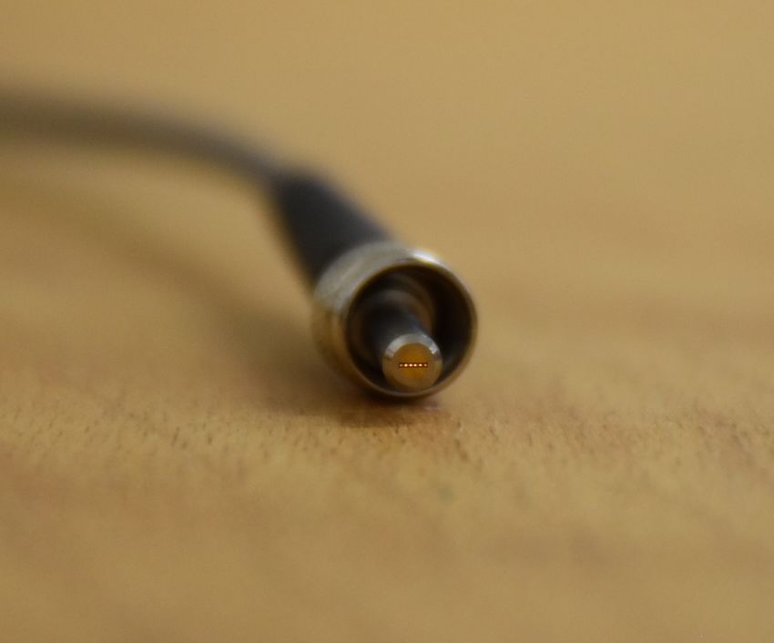
Research Article Journal of the Optical Society of America B 3
down the fiber link. To simplify design and production, the
MMFs are off-the-shelf fibers (Thorlabs FG105LCA). Their op-
tical properties (core diameter 105 µm, NA=0.22) were chosen
in order to reduce the core-to-core separation between the SMF
and MMFs, reducing the 3D printed lens dimensions.
B. Lens design
(a) 50µm 100µm
(b) Design and optimization of the MLR were performed using
the optical design software Zemax OpticStudio. To calculate the
MLR coupling efficiency into the SMF, the Physical Optics Propaga-
tion (POP) tool was employed, and for MMF coupling the Imag-
ing tool was used. POP uses Fourier and Fresnel propagation,
which is crucial when handling the near-Gaussian mode of the
SMF and the complex illumination pattern on the MLR. It is
computationally intensive however, so to design the shape of
50µm
(c) the lenses, the Imaging tool was used, which utilizes a ray tracing
Fiber algorithm to estimate the coupling efficiency into MMFs.
Bundle For our technology demonstrator, we aimed to have a strong
signal for tip-tilt sensing while also enabling high SMF coupling
efficiency. This will both increase the signal-to-noise ratio (SNR)
and also provide a signal in all six fibers within a reasonable
dynamic range. The diameter of the central aperture was chosen
Fanout to clip ∼13% of the light, reducing the maximum achievable SMF
3mm
(d) coupling efficiency with an idealized circular pupil from ∼80%
[31] to ∼65%. Using this aperture, the surface shape of the MLR
was then optimized to maximize the MMF coupling efficiency,
SMF MMFs weighted to favor on-axis beams with decreasing priority for
misalignment up to 100 µm (corresponding to ∼20 λ/D). The
surface shape of the individual lenses needs to provide suitable
optical power to focus the incoming clipped part of the beam into
the MMF. This was achieved by optimizing the spherical shape
Centroid and then adding corrections with both Zernike focal sag and
reconstruction
(e) separate conical constants in both directions. A strong optical
Science power was necessary to refract the beam from the inner edge
instrument of the microlens to the MMF. For this, polynomial corrections
were successively applied up to fourth order in the axis parallel
to the radial axis, no additional correction was applied in the
angular direction.
C. Lens manufacturing
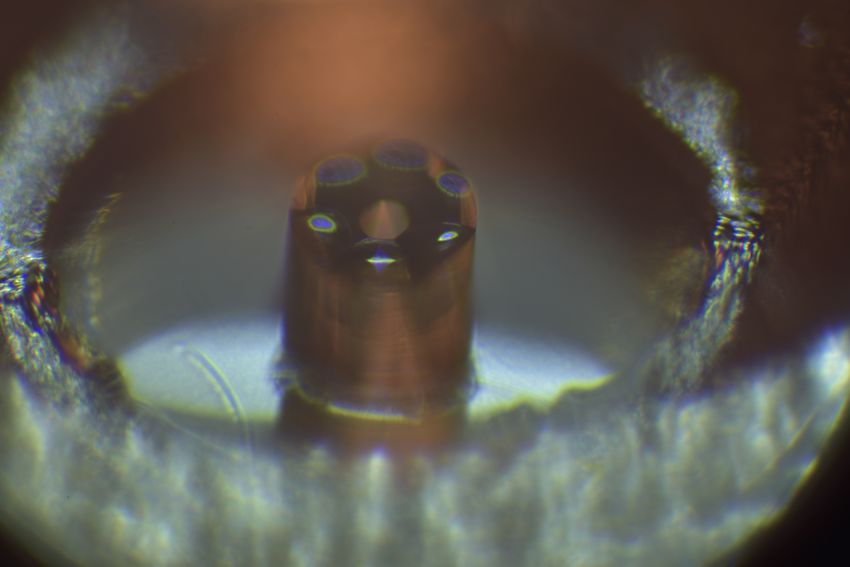
Fig. 2. Overview of the micro-lens ring tip-tilt sensor (MLR- The MLR was manufactured using two-photon polymerization
TT). (a) Schematics of the setup. The starlight (red) is coupled using a proprietary resin on the fiber tip [32], which allows
into the SMF (dark blue), while some light at the edges of the manufacturing of free-form lenses on small scales. Due to
the beam is clipped and refracted (orange beam) by the MLR the use of stages in the printing process, these structures can
(light blue) to be coupled into the sensing MMFs (dark green). take arbitrary shapes, limited by the need for an appropriate
The fibers are embedded in a fiber bundle that fans out into support structure and macroscopic forces. The printing is aided
a single SMF which then feeds the starlight into a science in- by back-illuminating the fiber bundle and yields sub-micron
strument and the six MMFs that are reformatted into a linear alignment precision [28] compensating for irregularities in the
array mounted in an SMA connector. The sensing fibers are bundle geometry. The process allows a precision of ∼100 nm
then re-imaged and the detected flux is used to reconstruct the and a root mean square (RMS) surface roughness of ∼10 nm.
centroid position of the telescope beam. (b) Microscope image The physical size was limited to the maximum build height of
of the MLR on the fiber bundle face, (c) microscope image of approximately 400 µm, due to the manufacturing stages and
back-illuminated fiber bundle, (d) sensing fiber output at the microscope objective numerical aperture (NA).
fiber connector, and (e) re-arranged detector signal for visual Once the MLR was printed on the fiber the FC/PC connector
examination of the reconstruction algorithm with the green was then placed within a bulkhead adapter (Thorlabs HAFC)
cross indicating the centroid position. for mechanical protection.
D. Laboratory sensor response
As the custom lenses belonging to the iLocater acquisition cam-
era were unavailable for laboratory experiments, the MLR-TT
sensor’s response was tested using commercial lenses. An SMF
illuminated by a 1050 nm SLED source (Thorlabs S5FC1050P),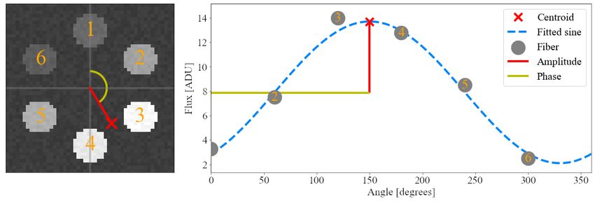
Research Article                                                                                               Journal of the Optical Society of America B    4

was apertured and a Thorlabs AC127-025-C lens was used to
produce an NA of 0.14, simulating the telescope’s Airy disc. The

                                                                        SMF coupling efficiency
experimental system provided a lower throughput than the final
                                                                                                                               Model: Bare SMF
on-sky experiment, due to lower image quality. The results in                                     75%
Fig. 3 show the sensor’s response to an gradually off-centered                                                                 Model: MLR-TT SMF
beam in the laboratory setup, both as modeled and as measured.                                                                 Lab.: MLR-TT SMF
The modeled SMF coupling efficiency (Fig. 3, top) includes Fres-                                  50%
nel reflection loss of 3.5% at both fiber input and output face.
The maximal achievable coupling efficiency within the MLR-TT
sensor’s SMF is measured at 59.9 ± 0.6% which is slightly lower                                   25%
than the expected value of 63.2% at the given wavelength. This
coupling efficiency then drops off slightly faster than expected
with an off-centered beam but features a slightly increased cou-                                  0%
pling for misalignment of up to 2.2 λ/D. The causes of this
                                                                                                  3%          Model: MMFs

                                                                        MMF sensor signal
behavior still to be understood but are likely due to fiber bundle
                                                                                                              Lab.: MMFs
and lens imperfections.
   The response of the sensing MMFs (Fig. 3, center) follows                                      2%
the modeled curves well, though the six sensing MMFs are not
evenly illuminated when the beam is centered. During align-
ment we found that the illumination pattern depends strongly
on the fiber alignment angle (pitch and yaw) and could not be
                                                                                                  1%
completely corrected. This can result from asymmetries in the
beam or uneven MMF properties such as irregular spacing or dif-
ferent fiber losses. In practice this is corrected by the calibration
                                                                                                  0%
                                                                                                              Model: Sum MMFs
                                                                        MMF sensor signal
routine (Sec. F).
                                                                                                  10%         Lab: Sum MMFs
    Laboratory results show the MLR couples 4.1% of the over-
all light into the MMFs when the beam is centered, which is
30% lower than the modeled value of 5.8% (this includes 11%
reflections and losses from the fiber and 8% from the lens). Inter-
estingly, this loss remains constant with respect to beam position                                5%
(Fig. 3, bottom) up to a centroid offset of ∼ 3 λ/D. We presume
that the remaining mismatch is due to a non-optimally shaped
lens surface. The ray approximation as described in Sec. B only
considers a central top-hat beam but fails to accurately account                                  0%
for the diffractive pattern that illuminates the lenses outside the                                     0.0   0.5    1.0      1.5     2.0                     2.5
                                                                                                                 Centroid offset [λ/D]
central beam.
    Theoretical throughput calculations and the corresponding
photon, sky background and camera noise associated with the
described system show that with this reduced sensor signal, a           Fig. 3. Modeled (solid lines) and measured (crosses) sensor re-
source with 8th magnitude in the J band can provide a SNR of 14         sponse as function of centroid offset. Top panel: The coupling
for each MMF output when running at 500 Hz. Simulations with            efficiency of the science SMF. Middle panel: The response of
the same pipeline as described in Sec. H show that this results in      the six sensing MMF as function of beam offset. Bottom panel:
an reconstruction accuracy of ∼0.1 λ/D in tip and tilt combined.        MLR-TT sensor signal summed over all six MMFs.
In this limiting case, performance is limited by read-out noise of
the detector.                                                           F. Reconstruction and calibration
                                                                        The reconstruction algorithm (see Fig. 4) calculates the MMF
                                                                        illumination and converts it to a physical centroid position. For
E. Signal processing                                                    this, the six fiber fluxes are ordered with their azimuthal coor-
                                                                        dinate and a sine function with angular period of 2π is fitted to
The output of the sensing MMFs was re-imaged with two lenses
                                                                        this signal. Three best fit parameters are obtained by this routine
mounted within a hybrid tube and cage mechanical system and
                                                                        (see Fig. 4):
directly attached to the lens interface of a First Light C-Red
2 InGaAs detector. This detector was chosen as it provides                      1. Offset, depending on both background signal and target
both a high frame rate (up to 16 kHz) and low read-out noise                       flux.
(34 e− ) with a pixel size of 15 µm. Each MMF illuminates a                     2. Amplitude, corresponding to the radial position of the
circular region on the detector with a diameter of 100 µm. For                     beam. Note, this is an arbitrary flux unit and the ampli-
each fiber, the 20 pixels with the highest SNR are selected and                    tude does therefore not directly yield the physical centroid
used for further processing. In laboratory tests, 20 pixels were                   position.
measured to provide a steady fraction of 80% of the flux and the
                                                                                3. Phase, corresponding to the azimuthal coordinate of the
best overall SNR. The detector data was then processed by the
                                                                                   centroid position.
Durham Adaptive optics Real-time Controller (DARC) [33, 34],
running on a consumer grade desktop computer.                                          Laboratory tests showed that this approach yields the most
Research Article Journal of the Optical Society of America B 5
reliable and stable output, less susceptible to noise than a simple for differing AO correction. To do this, an atmospheric wave-
center of mass (CoM) algorithm. front distortion of 1000 modes in combination with a correspond-
A calibration routine is used to correct the reconstructed ing AO system correcting 500 modes was modeled using the
centroid position for accurate loop feedback and run time di- HCIPy high contrast imaging simulation framework [35]. To
agnostics. It accounts for irregularities in the system such as allow an accurate comparison, the tip and tilt modes of the re-
asymmetries or misalignment of the MLR, transmission varia- sulting wavefront are replaced by the centroid positions that
tions within the fiber bundle and static aberrations in the PSF. were recorded during the on-sky observations.
For this, a circular motion is introduced with the tip-tilt mirror. These simulations are key as they allow us to understand our
The offset between the introduced and reconstructed azimuthal results and estimate the impact of residual AO aberrations and
coordinate and the factor between the respective radial coordi- their dominance with respect to other noise sources.
nates is approximated with individual best fit discrete Fourier
transforms (DFTs) of 5th order as a function of the azimuthal
coordinate. The obtained correction function is subsequently
3. RESULTS
applied to the measured centroid position. It should be noted We tested the MLR-TT on-sky in November 2019 at the LBT,
that this calibration routine is repeated for each target in order to using the left (SX) mirror of the telescope [15]. During the
remove slowly changing quasi-static aberrations (arising from run the Large Binocular Telescope Interferometer adaptive op-
effects such as mechanical flexure) and to include asymmetries tics (LBTI-AO) system was using the SOUL upgrade, which is
of the source itself such as companions or background sources. designed to produce an SR of up to 78% in I-band [36] under opti-
The interaction matrix is constructed by applying a linear mal conditions. For all observations the AO system was running
signal in both tip and tilt with the mirror and simultaneously at 1 kHz closed on 500 modes. Correction for AO non-common
measuring the centroid position. The resulting 2x2 matrix is then path aberration (NCPA) was performed before observations, but
inverted to obtain a reconstruction matrix, which can be used by otherwise there was no direct interaction between the MLR-TT
the control loop to convert the measured centroid position into sensor and LBTI-AO.
an feedback signal to command the tip-tilt mirror. We present the results from three on-sky targets, with a to-
tal of 8 datasets. All targets were chosen to be bright (< 6th
G. On-sky integration magnitude), marginalizing detector noise from the MLR-TT sen-
The MLR-TT sensor was integrated into the iLocater SX acqui- sor. Tab. 1 provides an overview of the targets, the AO loop
sition camera [15] that is fed by the Large Binocular Telescope performance, and the associated datasets.
Interferometer (LBTI). The optical path is illustrated in Fig. 5.
The iLocater acquisition camera receives the pupil from the tele-
scope (a), passes the wavelengths between 920 nm and 950 nm Table 1. Observed targets and datasets as well as observa-
(c) to its imaging channel equipped with an Andor focal plane tional seeing, estimated SR and and the status of the tip-tilt
camera (ANDOR Zyla 4.2 Plus, d), providing a sampling of correction loop.
6.1 pixels across the full width at half maximum (FWHM) of Target/dataset J- Seeing Est. SR Additional
the diffraction-limited PSF. This focal plane image is used as band (00 ) Tip-Tilt
reference for the centroid position, i.e. the tip-tilt. mag. control
iLocater’s native tip-tilt correction features a quad-cell photo
detector (Hamamatsu G6849-01 InGaAs, g), which is fed with HIP28634 /4 5.3 1.2-2.0 50 ± 6% MLR-TT
light picked off by a dichroic at 1.34-1.76 µm, (e) just before the /5 00 00 52 ± 7% None
final coupling optics. The quad-cell system can then feed an
error signal back to a fast tip-tilt mirror (nPoint RXY3-276, b) to HD12354 /1 5.9 1.0-1.4 67 ± 7% None
correct for tip-tilt. Alternatively, the mirror can be controlled by /2 00 00 67 ± 11% MLR-TT
the MLR-TT sensor to either introduce the required motions for
calibration (see Sec. F) or for correcting tip-tilt directly. HIP7981 /2 3.8 1.0-1.4 66 ± 4% MLR-TT
The science beam (0.97 − 1.31 µm) is focused by two custom /4 00 00 65 ± 4% MLR-TT
triplet lenses [15] to an f/3.7 beam on the SMF to match its
/5 00 00 65 ± 4% MLR-TT
MFD of 5.8 µm (1/e2 -intensity at 970 nm). The fiber mount can
be moved in 5 axes for alignment and to switch between three /6 00 00 65 ± 4% MLR-TT
independent fibers mounted at the instrument focal plane. These
are: the native iLocater SMF, a bare MMF (105 µm core diameter)
used for flux calibration, and the guest fiber port equipped with Each dataset includes three simultaneous measurements
the MLR-TT sensor (f). taken using iLocater and the MLR-TT sensor:
Fiber throughput is determined by measuring the output flux
• Andor focal plane frames (Sec. 2.G), taken at a frame rate of
from each fiber with the bare MMF serving as an incident flux
250 Hz. A symmetric 2D Gaussian function is fitted to the
reference. Output flux is measured with a FemtoWatt receiver
data in post processing and its calculated centroid used as a
[15]. The fiber bundle holding the six sensing MMFs is routed to
reference for PSF position. The SR in Tab. 1 was estimated
a separate opto-electric enclosure, housing the read-out optics
by fitting a Gaussian to the centroid corrected PSF and
and electronics.
taking the ratio between the normalized central intensities
of this fit and the expected telescope PSF as described in
H. Simulations of on-sky results Ref. 22. Due to the limited SNR of the individual frames,
To further investigate the performance of the sensor with our the SR calculations were smoothed by applying a moving
recorded on-sky conditions, we simulated the sensor response median algorithm covering 20 frames.Research Article Journal of the Optical Society of America B 6
Fig. 4. Illustration of the reconstruction routine with simulated noise. Left panel: Simulated detector image showing the six MMFs
(numbered 1-6 in orange) along with the reconstructed centroid of the PSF (red cross). Right panel: A graphical illustration of the
reconstruction routine. Here the six fiber fluxes (gray, numbered 1-6 in orange) are ordered by their azimuthal coordinate and a sine
function with angular period of 2π is fitted, giving the angle, amplitude and offset of the centroid.
• The reconstructed centroid position from the MLR-TT sen- Compared to the overall noise in these datasets (see Sec. D), the
sor (Sec. 2.F). Data were taken at a frame rate of 500 Hz. impact of the calibration is negligible.
In post processing the frames were interpolated and cross-
correlated to match the time reference of the Andor data.
Table 2. Improvement gained through the calibration rou-
• The SMF coupling efficiency was measured with the Fem- tine. RMS reconstruction error before and after applying the
toWatt receiver (Sec. 2.G). calibration is listed as well as the RMS shift determined af-
ter the application of the calibration routine.
A. Sensor calibration Target RMS error RMS error RMS calib.
As described in Sec. 2.F, the calibration pattern was generated no calib. calibrated shift
by introducing a circular motion on the tip-tilt mirror by issuing [λ/D] [λ/D] [λ/D]
open loop position commands. An example of the calibration
routine for target HIP7981 is shown in Fig. 6 for (a) the Andor ref- HIP28634 /cal. 0.54 0.50 0.23
erence centroid position, (b) the raw MLR-TT centroid position HD12354 /cal. 0.42 0.31 0.27
and (c) the calibrated centroid position.
During the calibration, the AO loop was closed, but no ad- HIP7981 /cal. 0.42 0.28 0.30
ditional tip-tilt correction was applied. Due to residual vibra-
tions at the telescope, the measured centroid positions show a
broadened pattern, which is averaged. The averaged centroid B. Closed-loop performance
positions are used to correct the reconstructed centroid for static In the datasets listed in Tab. 1, the acquired PSF centroid po-
asymmetries. sitions were used to drive the tip-tilt mirror. While the loop
For HIP7981, the reconstruction without calibration shows was operating stably, no improvement in SMF coupling was
an RMS error of 0.33 λ/D in tip and 0.26 λ/D in tilt (0.42 λ/D observed. The closed loop transfer function as seen by the MLR-
combined). After correction, this improves to 0.19 λ/D in tip TT sensor (Fig. 7, blue/orange) shows a significant rejection of
and 0.21 λ/D in tilt (0.28 λ/D combined) and appears random. frequencies below 15 Hz, however this is not seen in the Andor
The impact of the calibration on the reconstruction accuracy for reference camera (Fig. 7, green/red). Above 15 Hz both Andor
all targets is listed in Tab. 2, including the RMS shift that is ap- and MLR-TT show the same behavior, however the loop fails to
plied by the calibration. This shift corresponds to the correction correct for the faster disturbances. This suggests that the loop
that the calibration routine performs on the centroid position is not running at a high enough frequency for correction or the
which is seen as an improvement of the reconstructed centroid latency is too high.
position. The correction is seen to provide a more significant
improvement for the datasets with lower pre-calibration RMS C. Reconstruction accuracy
reconstruction error. This arises from a more precise measure- This significant mismatch between MLR-TT sensor and Andor
ment of the calibration pattern (corresponding to a thinner ring reference in evaluating the loop performance needs to be under-
in Fig. 6) that leads to a more accurate parametrization of the stood. For this, we analyze the accuracy with which the sensor
correction function. is able to reconstruct the centroid position. Fig. 8 shows the
For all other datasets listed in Tab. 1, the calibration was also centroid position for the Andor reference and the MLR-TT sen-
applied but did not provide a significant improvement. These sor for HD12354/1, as well as the corresponding reconstruction
datasets all feature a smaller dynamical range and the applied error. While the scatter of these values does not show any sys-
shift varied between 0.06 and 0.09 λ/D in tip and tilt combined. tematic patterns, the time series (cutout, bottom) shows that theResearch Article Journal of the Optical Society of America B 7
(g) (a) Andor
PSF centroid
(b) MLR-TT
raw (scaled)
(c) MLR-TT
calibrated
Quad-cell
3
Tilt [λ/D]
(f)
(e) 0
MLR-TT Tip-Tilt −3
Mirror
−3 0 3 −3 0 3 −3 0 3
Tip [λ/D] Tip [λ/D] Tip [λ/D]
(b)
(c) Fig. 6. Three scatter plots showing the on-sky calibration rou-
tine of target HIP7981. Shown are (a) the reference centroid
(a) position measured with the Andor focal plane camera, (b) the
MLR-TT reconstructed raw centroid position reconstructed
Andor (d) Light from LBTI
from the MLR-TT and (c) the calibrated MLR-TT centroid po-
sition (see Tab. 2). Initially the PSF is centered, then a circular
motion is introduced on the fast tip-tilt mirror. This movement
is not calibrated in λ/D and produces an elliptical shape in
the focal plane due to the angle of the tip-tilt mirror. The intro-
duced figure also features a central accumulation from before
and after the circular motion, as well as an introduced step
Fig. 5. Optical path of the experimental setup with the iLo- position seen as a separate patch to the top right of the circle.
cater acquisition camera at LBT (sizes are not to scale). (a) The
collimated AO corrected beam from LBTI is steered by a fast
tip-tilt mirror (b). A short-pass dichroic (c) transmits wave- construction error for tip and tilt combined as a function of
lengths between 920 and 950 nm to be imaged by the Andor the retrieved SR and is analogous to Fig. 10. For the lowest
focal plane camera (d). The science light is reflected by the simulated SRs of ∼50%, reconstruction accuracy is worse than
long-pass dichroic mirror (e) and focused into the MLR-TT 0.35 λ/D and improves to 0.16 λ/D for an SR of 80%. As with
sensor (f) and SMF. Light between 1.34-1.76 µm is transmitted the on-sky results (cf. Fig. 10), the data are well fit by a linear
and imaged on the quad-cell (g) that can be used in closed- trend, with a slope of −0.72 ± 0.05 λ/D. For completeness, we
loop to correct for tip-tilt vibrations. have also simulated the reconstruction error for a flat wavefront
(Fig. 11, yellow marker) which shows a reconstruction error of
less than 0.05 λ/D.
sensor is indeed able to track the centroid position. The residual
error features a mismatch, amounting to 0.19 λ/D RMS in both 4. DISCUSSION
tip and tilt.
The time series of the error suggests a strong low-frequency In the preceding section we presented the on-sky performance of
component. The power spectral density (PSD) of the MLR-TT the MLR-TT sensor. Whilst able to track incident beam motions,
sensor tracks this behavior very well (see Fig. 9), with the sensor the sensor was unable to improve fiber coupling performance
PSD tracking the features of the reference centroid very accu- with our current AO loop. The sensor also shows limitations in
rately above 10 Hz. Residuals below 10 Hz are calculated to the overall performance which can be achieved due to the effects
account for approximately 50% of the combined tip-tilt error, of residual aberrations. The causes and solutions are discussed
while residuals between 10 and 20 Hz contribute less than 20%. in this section.
D. Impact of AO performance A. Sensor reconstruction limitations
Fig. 10 shows the combined tip-tilt reconstruction error for all As shown in Fig. 10, the sensor was able to reconstruct the
datasets as a function of estimated SR. Note that all datasets centroid position to an accuracy of 0.27 λ/D combined tip-tilt
feature similar RMS centroid values (∼λ/D). RMS. The majority of this error (50%) originates in frequencies
The wavefront correction varies significantly between the below 10 Hz and depends strongly on the estimated SR. To
datasets and within individual datasets, with subsets featuring ascertain the cause of this error, we presented optical simulations
SRs as low as 40% and reaching up to 80%. The reconstruction with differing SR in Sec. 3.E. The simulations show the same
accuracy shows a strong dependency on the SR and improves trend with a slightly flatter linear fit. The discrepancy can by
significantly with increasing SR. The best reconstruction shows attributed to a number of additional noise sources that occur
a combined tip-tilt RMS of 0.27 λ/D while the worst reconstruc- within the measurements. These alternative sources include
tion reaches an RMS error of 0.5 λ/D. A linear fit yields a slope detector noise, reconstruction algorithm error, NCP vibrations,
of −0.95 ± 0.20 λ/D, an improvement in RMS reconstruction flux variations, and noise in the measurements of the reference
accuracy of ∼0.1 λ/D per 10% increase in SR. centroid. While we investigated these factors during analysis,
the current system is most strongly impacted by the effects of
E. On-sky sensor simulations residual aberrations. For future versions of the sensor we aim to
AO simulations as described in Sec. H were performed to re- understand the exact contributions that these noise terms have
construct the sensor operation. Fig. 11 shows the resulting re- on the reconstruction accuracy.Research Article Journal of the Optical Society of America B 8
(a) Andor (b) MLR-TT (c) Reconst. error
101
Transfer function [λ2 /(D2 Hz)]
1
Tilt [λ/D]
±0.43
±0.41
±0.19
0
100 −1 ±0.19
±0.29 ±0.32
−1 0 1 −1 0 1 −1 0 1
10−1 Tip [λ/D] Tip [λ/D] Tip [λ/D]
10−2
1 1
Tilt [λ/D]
Tip [λ/D]
10−3 0 0
MLR/Tip Andor/Tip
MLR/Tilt Andor/Tilt −1 −1
10−4 Andor MLR-TT Error
0 10 20 30 1 1
Error Tilt [λ/D]
Error Tip [λ/D]
Frequency [Hz] 0 0
Fig. 7. Closed loop transfer function when stabilizing the
−1 −1
beam with the MLR-TT sensor for datasets HIP28634/4
(closed loop) and HIP28634/5. Below ∼10 Hz, the MLR-TT
2.0 2.2 2.4 2.6 2.8 2.2 2.4 2.6 2.8 3.0
sensor (blue, yellow) detects a different frequency rejection Time [s] Time [s]
than the Andor reference (green, red), whilst above 10 Hz the
transfer functions agree well. Fig. 8. Sensor reconstruction accuracy shown graphically. Top
panels: Time series of (Left) the centroid position measured
by the Andor focal plane camera, (Center) the position re-
To further investigate the impact of wavefront aberrations
constructed with the MLR-TT and (Right) the error in the
on the MLR-TT sensor, in future laboratory testing and on-sky
reconstruction by taking the difference between the former
experiments, we intend to acquire additional metrology data to
two datasets. Bottom panels: Time series graphs of the same
identify other effects driving performance. This will allow us to
dataset for: (Top) Comparison of the centroid x-position for
optimize the MLR-TT reconstruction algorithm to account for
(tip, left) and y-position (tilt, right) of Andor reference (blue)
the observed aberrations and possibly even reconstruct Zernike
and MLR-TT (red), and (Bottom) the corresponding recon-
modes beyond tip and tilt.
struction error (green) from their difference.
B. Loop performance
As illustrated in Fig. 10, under the best conditions experienced, rates, the sensor also needs less light for operation, increasing
the reconstruction accuracy of the sensor provided a combined the limiting sensing magnitude and the light available for the
RMS error of 0.27 λ/D. Assuming an ideal control system, this science instrument.
would provide correction with an RMS error 1.5 times lower
than the existing quad-cell system. With our current control C. Sensor optimization
system, this is reduced significantly due to latency and meant To control the amount of noise that is induced by residual AO
the loop was only able to reject frequencies up to 15-20 Hz. The aberrations, the lens design can be tuned for future devices. As
control system therefore needs to be optimized in order to allow the shape of the MLR surface is set by the need to efficiently
a better correction of the tip-tilt disturbance which holds the couple light into the MMFs, the height of the lens and the size of
most power in frequencies between 10 and 20 Hz (see Fig. 9). the central aperture then become the most important variables.
As shown in Fig. 9, most of the noise in the reconstruction Both parameters control the distance from the focal plane where
occurs below 10 Hz. The main goal will be to optimize the MLR- the telescope beam is sensed and by varying them the impact of
TT sensor software (Sec. A) and hardware design (Sec. C) to aberrations in the system changes.
improve its performance in this regime. Even without additional By sampling the beam closer to the fiber focal plane, the
precision, the loop can be tuned to filter this frequency range MLR-TT sensor will use an intensity distribution more similar
or another sensor designed to supress vibrations in the range to the PSF for sensing, which depends mostly on the phase of
1-10 Hz can be added. Alternatively, the MLR-TT sensor may be the wavefront at the pupil. As the height of the MLR increases,
used to only detect slow beam drift below 1 Hz. Any residual the beam enters the Fresnel regime and the sensor is therefore
aberrations will average out over long timescales (>1 second) also affected by variations in the pupil intensity that arise from
and the sensor can be optimized to measure slow mechanical scintillation and pupil instability. Fully analyzing this parameter
drift resulting from e.g. gravitational flexures. This would focus space will be crucial for future sensor optimization.
the sensor on utilizing one of its main advantage, namely that it The size of the lens ring aperture determines how much
is virtually free from NCP effects. When running at lower frame of the beam’s central core is diverted to the sensor. As theResearch Article Journal of the Optical Society of America B 9
-1 0 1 -1 0 1 -1 0 1 -1 0 1 -1 0 1 -1 0 1 -1 0 1 -1 0 1
1
Tip/Tilt
RMS recon. error combined [λ/D] [λ/D]
101 101
0
-1
PSD Tilt [λ2 /(D2 Hz)]
PSD Tip [λ2 /(D2 Hz)]
0 0
10 10
10−1 10−1 HIP28634/4 HIP7981/5
0.6
−2 −2
HIP28634/5 HIP7981/6
10 10
HIP7981/2 HD12354/2
10−3 10−3 0.5 HIP7981/4 HD12354/1
Andor MLR-TT Error
101 101
PSD Error Tilt [λ2 /(D2 Hz)]
PSD Error Tip [λ2 /(D2 Hz)]
0
0.4
10 100
10−1 10−1
0.3
−2
10 10−2
10−3 10−3 0.2
0 20 40 60 80 20 40 60 80 100
0.4 0.5 0.6 0.7 0.8
Frequency [Hz] Frequency [Hz]
Estimated Strehl Ratio
Fig. 9. Power spectral density (PSD) for HD12354/1 of the sig-
nal shown in Fig. 8. (Top) PSD of centroid x-position (tip, left) Fig. 10. On-sky sensor performance. Main panel: Reconstruc-
and y-position (tilt, right) of MLR-TT (red) compared to the tion accuracy as a function of estimated Strehl ratio (SR) for
Andor reference (blue), (Bottom) the PSD of the correspond- these datasets. Cross marks in the main plot represent the
ing reconstruction error (green) for tip and tilt. Most of the mean and error for each dataset, while the circles in the sub-
vibrational power lies between 10 and 20 Hz, whilst most of plots correspond to subsets with different estimated SRs, with
the reconstruction error is in the low frequencies (< 10 Hz). the size of the circle representing the number of frames in each
set. The dashed lines show the fitting error. Top panels: The
centroid reconstruction error scatter plot for each analyzed
edges of the beam are more susceptible to higher order modes dataset.
and asymmetries, using more of the beam’s core will result in
more reliable measurements. However, this will also reduce
the fraction of light available for science measurements. This
trade off is the key design choice that will be determined by tures a very small opto-mechanical footprint and degrades the
future use cases and implementations. In addition to the size maximum single-mode fiber coupling efficiency by 15%, which
of the central aperture, the NA can be used to slightly change is comparable to typical losses due to beam aberrations.
the ratio between sensor signal and SMF coupling. Given the
right optical system, it would be possible to perform individual We showed that the fundamental principle works well and
adjustments of this trade off for each observed target. the sensor is able to reach a maximum reconstruction accuracy
of 0.19 λ/D in each tip and tilt, however, the system was not able
D. Future applications to improve single-mode fiber coupling efficiency. The majority
The system presented in this work was optimized to be used of the vibration was measured in frequencies between 10-20 Hz,
with the iLocater acquisition camera at the LBT, however there but the majority of the reconstruction error was shown to occur
are other diffraction-limited systems where the technology can in low frequencies between 1-10 Hz. This error in reconstructing
find application. As discussed in Sec. A, the performance is the centroid depended strongly on estimated Strehl ratio (SR)
limited by residual AO aberrations, and thus the most beneficial and subsequent simulations were able to recreate this trend,
application will be with systems that feature as little residual suggesting that residual aberrations were the dominating noise
wavefront aberrations as possible. source that limited performance.
Besides current and future ExAO system at large observato-
ries, the MLR-TT sensor can have an advantage for small obser- These findings will help to tune both the optical design and
vatories, free-space optical communication systems and space reconstruction algorithm to improve the centroid measurements
based applications that employ diffraction-limited telescopes. In and to reduce the impact of residual aberrations. Alternatively,
these systems, the sensor can be integrated in a very compact the respective frequency range can be filtered or corrected using
fashion without the need for additional optical components in another sensor to minimize its impact.
the optical train reducing complexity and mechanical footprint.
We conclude that the MLR-TT sensor is best suited for appli-
cations requiring fast correction with low higher-order wave-
5. CONCLUSION
front distortions while benefiting from its compact nature. This
We presented the first on-sky results of our novel 3D-printed, includes extreme adaptive optics systems, compact systems at
fiber-based tip-tilt sensor (MLR-TT). The sensor was tested with small diffraction-limited telescopes and space based applica-
the iLocater acquisition camera at the Large Binocular Telescope tions. We also note that the MLR-TT sensor operates very close
in November 2019. The system consists of a 3D-printed micro- to the fiber coupling surface, it is free of non-common path aber-
lens ring that uses six multi-mode fibers to reconstruct the cen- ration and can therefore be used to track drifts and perform
troid position, while providing an almost unobscured aperture guiding in a closed-loop system where calibration between the
where a science single-mode fiber is positioned. This concept fea- wavefront sensor and fiber is difficult.Research Article Journal of the Optical Society of America B 10
REFERENCES
-1 0 1 -1 0 1 -1 0 1 -1 0 1 -1 0 1 -1 0 1
1 1. J.-L. Beuzit, M. Feldt, K. Dohlen, D. Mouillet, P. Puget, F. Wildi, L. Abe,
Tip/Tilt [λ/D]
0 J. Antichi, A. Baruffolo, P. Baudoz, A. Boccaletti, M. Carbillet, J. Charton,
-1 R. Claudi, M. Downing, C. Fabron, P. Feautrier, E. Fedrigo, T. Fusco, J.-
1 L. Gach, R. Gratton, T. Henning, N. Hubin, F. Joos, M. Kasper, M. Lan-
0 glois, R. Lenzen, C. Moutou, A. Pavlov, C. Petit, J. Pragt, P. Rabou, F. Ri-
-1 gal, R. Roelfsema, G. Rousset, M. Saisse, H.-M. Schmid, E. Stadler,
C. Thalmann, M. Turatto, S. Udry, F. Vakili, and R. Waters, “SPHERE:
0.6 RMS=0.16λ RMS=0.07λ a ’Planet Finder’ instrument for the VLT,” (2008), p. 701418.
RMS=0.14λ RMS=0.06λ 2. S. Esposito, A. Riccardi, E. Pinna, A. Puglisi, F. Quirós-Pacheco, C. Ar-
RMS=0.13λ RMS=0.05λ
RMS recon. error combined [λ/D]
0.5 cidiacono, M. Xompero, R. Briguglio, G. Agapito, L. Busoni, L. Fini,
RMS=0.12λ RMS=0.03λ J. Argomedo, A. Gherardi, G. Brusa, D. Miller, J. C. Guerra, P. Stefanini,
RMS=0.10λ RMS=0.02λ and P. Salinari, “Large Binocular Telescope Adaptive Optics System:
0.4 RMS=0.08λ RMS=0.00λ new achievements and perspectives in adaptive optics,” (2011), p.
814902.
3. B. Macintosh, J. R. Graham, P. Ingraham, Q. Konopacky, C. Marois,
0.3
M. Perrin, L. Poyneer, B. Bauman, T. Barman, A. S. Burrows, A. Card-
well, J. Chilcote, R. J. De Rosa, D. Dillon, R. Doyon, J. Dunn, D. Erik-
0.2 son, M. P. Fitzgerald, D. Gavel, S. Goodsell, M. Hartung, P. Hibon,
P. Kalas, J. Larkin, J. Maire, F. Marchis, M. S. Marley, J. McBride,
M. Millar-Blanchaer, K. Morzinski, A. A. Norton, B. R. Oppenheimer,
0.1 D. D. Palmer, J. Patience, L. Pueyo, F. Rantakyro, N. Sadakuni, L. Sad-
dlemyer, D. Savransky, A. Serio, R. Soummer, A. Sivaramakrishnan,
I. Song, S. Thomas, J. K. Wallace, S. Wiktorowicz, S. Wolff, R. J. D.
0.0
Rosa, D. Dillon, R. Doyon, J. Dunn, D. Erikson, M. P. Fitzgerald,
0.4 0.6 0.8 1.0 D. Gavel, S. Goodsell, M. Hartung, P. Hibon, P. Kalas, J. Larkin, J. Maire,
Estimated Strehl Ratio F. Marchis, M. S. Marley, J. McBride, M. Millar-Blanchaer, K. Morzinski,
A. A. Norton, B. R. Oppenheimer, D. D. Palmer, J. Patience, L. Pueyo,
Fig. 11. Synthetic MLR-TT sensor performance derived from F. Rantakyro, N. Sadakuni, L. Saddlemyer, D. Savransky, A. Serio,
AO simulations, plotted to be comparable to Fig. 10. Main R. Soummer, A. Sivaramakrishnan, I. Song, S. Thomas, J. K. Wallace,
panel: Reconstruction accuracy as a function of Strehl ra- S. Wiktorowicz, S. Wolff, R. J. De Rosa, D. Dillon, R. Doyon, J. Dunn,
tio (SR) for AO simulations with varying residual aberration D. Erikson, M. P. Fitzgerald, D. Gavel, S. Goodsell, M. Hartung, P. Hi-
strength labeled with their RMS wavefront error. Crosses rep- bon, P. Kalas, J. Larkin, J. Maire, F. Marchis, M. S. Marley, J. McBride,
M. Millar-Blanchaer, K. Morzinski, A. A. Norton, B. R. Oppenheimer,
resent overall mean and error for each data set, while the
D. D. Palmer, J. Patience, L. Pueyo, F. Rantakyro, N. Sadakuni, L. Sad-
circles correspond to subsets binned by SR, with the size of dlemyer, D. Savransky, A. Serio, R. Soummer, A. Sivaramakrishnan,
the circle representing the number of frames in each set.The I. Song, S. Thomas, J. K. Wallace, S. Wiktorowicz, and S. Wolff, “First
dashed lines show the fitting error. Top panels: Centroid re- light of the Gemini Planet Imager,” Proc. Natl. Acad. Sci. United States
construction error scatter for the individual datasets. Am. 111, 12661–12666 (2014).
4. N. Jovanovic, F. Martinache, O. Guyon, C. Clergeon, G. Singh, T. Kudo,
V. Garrel, K. Newman, D. Doughty, J. Lozi, J. Males, Y. Minowa,
Y. Hayano, N. Takato, J. Morino, J. Kuhn, E. Serabyn, B. Norris, P. Tuthill,
6. BACKMATTER
G. Schworer, P. Stewart, L. Close, E. Huby, G. Perrin, S. Lacour,
L. Gauchet, S. Vievard, N. Murakami, F. Oshiyama, N. Baba, T. Matsuo,
J. Nishikawa, M. Tamura, O. Lai, F. Marchis, G. Duchene, T. Kotani,
Acknowledgments. P.H., R. J. H., and A.Q. are supported by the and J. Woillez, “The subaru coronagraphic extreme adaptive optics
Deutsche Forschungsgemeinschaft (DFG) through project 326946494, system: enabling high-contrast imaging on solar-system scales,” Publ.
’Novel Astronomical Instrumentation through photonic Reformatting’. Astron. Soc. Pac. 127, 890 (2015).
This project has received support from the European Union’s Hori- 5. J. R. P. Angel, “Ground-based imaging of extrasolar planets using
zon 2020 research and innovation program under grant agreement No adaptive optics,” Nature 368, 203–207 (1994).
730890. NAB, AGB and TJM acknowledge funding from UKRI Sci- 6. A. Bechter, J. Crass, R. Ketterer, J. R. Crepp, R. O. Reynolds,
ence and Technology Facilities Council (ST/T000244/1: NAB, TJM ; E. Bechter, P. Hinz, F. Pedichini, M. Foley, E. Runburg, E. E. Onuma,
ST/P000541/1: AGB, NAB, TJM). S. Gaudi, G. Micela, I. Pagano, and C. E. Woodward, “On-sky single-
This research made use of HCIPy, an open-source object-oriented frame- mode fiber coupling measurements at the Large Binocular Telescope,”
work written in Python for performing end-to-end simulations of high- (2016), p. 99092X.
contrast imaging instruments [35], Astropy, a community-developed 7. J. R. Crepp, J. Crass, D. King, A. Bechter, E. Bechter, R. Ketterer,
core Python package for Astronomy [37, 38], Numpy [39] and Matplotlib R. Reynolds, P. Hinz, D. Kopon, D. Cavalieri, L. Fantano, C. Koca, E. On-
[40]. uma, K. Stapelfeldt, J. Thomes, S. Wall, S. Macenka, J. McGuire, R. Ko-
We thank the reviewers for the time improving this manuscript and rniski, L. Zugby, J. Eisner, B. S. Gaudi, F. Hearty, K. Kratter, M. Kuch-
Romain Laugier for useful information about single-mode fiber (SMF) ner, G. Micela, M. Nelson, I. Pagano, A. Quirrenbach, C. Schwab,
use in interferometry. M. Skrutskie, A. Sozzetti, C. Woodward, and B. Zhao, “iLocater: a
diffraction-limited Doppler spectrometer for the Large Binocular Tele-
scope,” (2016), p. 990819.
Disclosures. The authors declare no conflicts of interest.
8. S. Y. Haffert, R. J. Harris, A. Zanutta, F. A. Pike, A. Bianco, E. Redaelli,
A. Benoît, D. G. MacLachlan, C. A. Ross, I. Gris-Sánchez et al.,
Data Availability Statement. Data underlying the results pre- “Diffraction-limited integral-field spectroscopy for extreme adaptive op-
sented in this paper are not publicly available at this time but may tics systems with the multicore fiber-fed integral-field unit,” J. Astron.
be obtained from the authors upon reasonable request. Telesc. Instruments, Syst. 6, 045007 (2020).Research Article Journal of the Optical Society of America B 11
9. V. Coudé du Foresto, “Integrated Optics in Astronomical Interferometry,” E. Kambe, M. Ikoma, Y. Hori, H. Genda, A. Fukui, Y. Fujii, H. Harakawa,
Symp. - Int. Astron. Union 158, 261–271 (1994). M. Hayashi, M. Hidai, M. Machida, T. Matsuo, T. Nagata, M. Ogihara,
10. Le Bouquin, J.-B., Berger, J.-P., Lazareff, B., Zins, G., Haguenauer, P., H. Takami, N. Takato, H. Terada, J. Kwon, D. Oh, K. Kashiwagi, T. Naka-
Jocou, L., Kern, P., Millan-Gabet, R., Traub, W., Absil, O., Augereau, jima, H. Baba, and G. Olivier, “The infrared Doppler (IRD) instrument
J.-C., Benisty, M., Blind, N., Bonfils, X., Bourget, P., Delboulbe, A., for the Subaru telescope: instrument description and commissioning
Feautrier, P., Germain, M., Gitton, P., Gillier, D., Kiekebusch, M., Kluska, results,” in Ground-based and Airborne Instrumentation for Astronomy
J., Knudstrup, J., Labeye, P., Lizon, J.-L., Monin, J.-L., Magnard, Y., VII, vol. 1070211 H. Takami, C. J. Evans, and L. Simard, eds. (SPIE,
Malbet, F., Maurel, D., Ménard, F., Micallef, M., Michaud, L., Montagnier, 2018), p. 37.
G., Morel, S., Moulin, T., Perraut, K., Popovic, D., Rabou, P., Rochat, 19. D. Mawet, P. Wizinowich, R. Dekany, M. Chun, D. Hall, S. Cetre,
S., Rojas, C., Roussel, F., Roux, A., Stadler, E., Stefl, S., Tatulli, E., O. Guyon, J. K. Wallace, B. Bowler, M. Liu, G. Ruane, E. Serabyn,
and Ventura, N., “Pionier: a 4-telescope visitor instrument at vlti,” A & R. Bartos, J. Wang, G. Vasisht, M. Fitzgerald, A. Skemer, M. Ireland,
A 535, A67 (2011). J. Fucik, J. Fortney, I. Crossfield, R. Hu, and B. Benneke, “Keck Planet
11. S. Gillessen, F. Eisenhauer, G. Perrin, W. Brandner, C. Straubmeier, Imager and Characterizer: concept and phased implementation,” in
K. Perraut, A. Amorim, M. Schöller, C. Araujo-Hauck, H. Bartko, Adaptive Optics Systems V, vol. 9909 E. Marchetti, L. M. Close, and
H. Baumeister, J.-P. Berger, P. Carvas, F. Cassaing, F. Chapron, E. Cho- J.-P. Véran, eds. (2016), p. 99090D.
quet, Y. Clenet, C. Collin, A. Eckart, P. Fedou, S. Fischer, E. Gendron, 20. J. Milli, D. Mouillet, J.-L. Beuzit, J.-F. Sauvage, T. Fusco, P. Bourget,
R. Genzel, P. Gitton, F. Gonte, A. Gräter, P. Haguenauer, M. Haug, M. Kasper, K. Tristam, C. Reyes, J. H. Girard, A. Telle, C. Pannetier,
X. Haubois, T. Henning, S. Hippler, R. Hofmann, L. Jocou, S. Kellner, F. Cantalloube, Z. Wahhaj, D. Mawet, A. Vigan, and M. N’Diaye, “Low
P. Kervella, R. Klein, N. Kudryavtseva, S. Lacour, V. Lapeyrere, W. Laun, wind effect on VLT/SPHERE: impact, mitigation strategy, and results,”
P. Lena, R. Lenzen, J. Lima, D. Moratschke, D. Moch, T. Moulin, in Adaptive Optics Systems VI, D. Schmidt, L. Schreiber, and L. M.
V. Naranjo, U. Neumann, A. Nolot, T. Paumard, O. Pfuhl, S. Rabien, Close, eds. (SPIE, 2018), p. 83.
J. Ramos, J. M. Rees, R.-R. Rohloff, D. Rouan, G. Rousset, A. Sevin, 21. J. Lozi, O. Guyon, N. Jovanovic, N. Takato, G. Singh, B. Norris, H. Okita,
M. Thiel, K. Wagner, M. Wiest, S. Yazici, and D. Ziegler, “GRAVITY: a T. Bando, and F. Martinache, “Characterizing vibrations at the subaru
four-telescope beam combiner instrument for the VLTI,” in Proc. SPIE, telescope for the subaru coronagraphic extreme adaptive optics instru-
vol. 7734 (2010), p. 77340Y. ment,” J. Astron. Telesc. Instruments, Syst. 4, 049001 (2018).
12. N. Cvetojevic, E. Huby, G. Martin, S. Lacour, F. Marchis, J. Lozi, N. Jo- 22. A. J. Bechter, J. Crass, J. Tesch, J. R. Crepp, and E. B. Bechter,
vanovic, S. Vievard, O. Guyon, L. Gauchet, G. Perrin, G. Duchêne, and “Characterization of Single-mode Fiber Coupling at the Large Binocular
T. Kotani, “FIRST, the pupil-remapping fiber interferometer at Subaru Telescope,” Publ. Astron. Soc. Pac. 132, 015001 (2019).
telescope: towards photonic beam-combination with phase control and 23. S. Esposito, E. Marchetti, R. Ragazzoni, A. Baruffolo, J. Farinato, L. Fini,
on-sky commissioning results (Conference Presentation),” in Optical A. Ghedina, P. Ranfagni, and A. Riccardi, “Laboratory characterization
and Infrared Interferometry and Imaging VI, vol. 10701 M. J. Creech- of an APD-based tip-tilt corrector,” in Proceedings of SPIE - The In-
Eakman, P. G. Tuthill, and A. Mérand, eds., International Society for ternational Society for Optical Engineering, vol. 3126 R. K. Tyson and
Optics and Photonics (SPIE, 2018). R. Q. Fugate, eds. (1997), p. 378.
13. Martinod, M. A., Mourard, D., Bério, P., Perraut, K., Meilland, A., Bailet, 24. M. Glück, J.-U. Pott, and O. Sawodny, “Investigations of an
C., Bresson, Y., ten Brummelaar, T., Clausse, J. M., Dejonghe, J., Accelerometer-based Disturbance Feedforward Control for Vibration
Ireland, M., Millour, F., Monnier, J. D., Sturmann, J., Sturmann, L., and Suppression in Adaptive Optics of Large Telescopes,” Publ. Astron.
Tallon, M., “Fibered visible interferometry and adaptive optics: Friend Soc. Pac. 129, 065001 (2017).
at chara,” A & A 618, A153 (2018). 25. M. Lippa, S. Gillessen, N. Blind, Y. Kok, Ş. Yazici, J. Weber, O. Pfuhl,
14. N. Cvetojevic, N. Jovanovic, S. Gross, B. Norris, I. Spaleniak, M. Haug, S. Kellner, E. Wieprecht, F. Eisenhauer, R. Genzel, O. Hans,
C. Schwab, M. J. Withford, M. Ireland, P. Tuthill, O. Guyon, F. Mar- F. Haußmann, D. Huber, T. Kratschmann, T. Ott, M. Plattner, C. Rau,
tinache, and J. S. Lawrence, “Modal noise in an integrated photonic E. Sturm, I. Waisberg, E. Wiezorrek, G. Perrin, K. Perraut, W. Brand-
lantern fed diffraction-limited spectrograph,” Opt. Express 25, 25546 ner, C. Straubmeier, and A. Amorim, “The metrology system of the
(2017). VLTI instrument GRAVITY,” in Optical and Infrared Interferometry and
15. J. Crass, A. Bechter, B. Sands, D. King, R. Ketterer, M. Engstrom, Imaging V, vol. 9907 F. Malbet, M. J. Creech-Eakman, and P. G. Tuthill,
R. Hamper, D. Kopon, J. Smous, J. R. Crepp, M. Montoya, O. Dur- eds. (2016), p. 990722.
ney, D. Cavalieri, R. Reynolds, M. Vansickle, E. Onuma, J. Thomes, 26. M. Corrigan, R. J. Harris, R. R. Thomson, D. G. MacLachlan,
S. Mullin, C. Shelton, K. Wallace, E. Bechter, A. Vaz, J. Power, G. Rah- J. Allington-Smith, R. Myers, and T. Morris, “Wavefront sensing using a
mer, and S. Ertel, “Final Design and On-Sky Testing of the iLocater SX photonic lantern,” in SPIE Astronomical Telescopes+ Instrumentation,
Acquisition Camera: Broadband Single-Mode Fiber Coupling,” Mon. (International Society for Optics and Photonics, 2016), pp. 990969–
Notices Royal Astron. Soc. 18, 1–18 (2020). 990969.
16. A. Vigan, J.-L. Beuzit, K. Dohlen, D. Mouillet, G. Otten, E. Muslimov, 27. B. R. Norris, J. Wei, C. H. Betters, A. Wong, and S. G. Leon-Saval,
M. Philipps, R. Dorn, M. Kasper, I. Baraffe, A. Reiners, and U. See- “An all-photonic focal-plane wavefront sensor,” Nat. Commun. 11, 1–9
mann, “Bringing high-spectral resolution to VLT/SPHERE with a fiber (2020).
coupling to VLT/CRIRES+,” in Ground-based and Airborne Instrumen- 28. P.-I. Dietrich, R. J. Harris, M. Blaicher, M. K. Corrigan, T. J. Morris,
tation for Astronomy VII, H. Takami, C. J. Evans, and L. Simard, eds. W. Freude, A. Quirrenbach, and C. Koos, “Printed freeform lens ar-
(SPIE, 2018), p. 115. rays on multi-core fibers for highly efficient coupling in astrophotonic
17. T. Feger, C. Bacigalupo, T. R. Bedding, J. Bento, D. W. Coutts, M. J. systems,” Opt. Express 25, 18288 (2017).
Ireland, Q. A. Parker, A. Rizzuto, and I. Spaleniak, “RHEA: the ultra- 29. P. Hottinger, R. J. Harris, P.-I. Dietrich, M. Blaicher, M. Glück, A. Bechter,
compact replicable high-resolution exoplanet and Asteroseismology J.-U. Pott, O. Sawodny, A. Quirrenbach, J. Crass, and C. Koos, “Micro-
spectrograph,” in Ground-based and Airborne Instrumentation for As- lens arrays as tip-tilt sensor for single mode fiber coupling,” in Advances
tronomy V, vol. 9147 S. K. Ramsay, I. S. McLean, and H. Takami, eds. in Optical and Mechanical Technologies for Telescopes and Instrumen-
(2014), p. 91477I. tation III, vol. 1070629 R. Geyl and R. Navarro, eds. (SPIE, 2018),
18. T. Kotani, M. Tamura, H. Suto, J. Nishikawa, A. Ueda, M. Kuzuhara, p. 77.
M. Omiya, J. Hashimoto, T. Kurokawa, T. Kokubo, T. Mori, Y. Tanaka, 30. P. Hottinger, R. J. Harris, P. I. Dietrich, M. Blaicher, A. Bechter, J. Crass,
M. Konishi, T. Kudo, T. Hirano, B. Sato, S. Jacobson, K. Hodapp, M. Glück, J. U. Pott, N. A. Bharmal, A. Basden, T. J. Morris, C. Koos,
D. Hall, M. Ishizuka, H. Kawahara, Y. Ikeda, T. Yamamuro, H. Ishikawa, O. Sawodny, and A. Quirrenbach, “Focal plane tip-tilt sensing for im-
K. Hosokawa, N. Kusakabe, J.-I. Morino, S. Nishiyama, N. Jovanovic, proved single-mode fiber coupling using a 3D-printed microlens-ring,”
W. Aoki, T. Usuda, N. Narita, E. Kokubo, Y. Hayano, H. Izumiura, in Proceedings of AO4ELT6, (2019).You can also read