Past Disturbance-Present Diversity: How the Coexistence of Four Different Forest Communities within One Patch of a Homogeneous Geological ...
←
→
Page content transcription
If your browser does not render page correctly, please read the page content below
Article
Past Disturbance–Present Diversity: How the Coexistence
of Four Different Forest Communities within One Patch
of a Homogeneous Geological Substrate Is Possible
Piotr T. Zaniewski * , Artur Obidziński, Wojciech Ciurzycki and Katarzyna Marciszewska

                                          Department of Forest Botany, Institute of Forest Sciences, Warsaw University of Life Sciences,
                                          Nowoursynowska 159, 02-776 Warsaw, Poland; artur_obidzinski@sggw.edu.pl (A.O.);
                                          wojciech_ciurzycki@sggw.edu.pl (W.C.); katarzyna_marciszewska@sggw.edu.pl (K.M.)
                                          * Correspondence: piotr_zaniewski@sggw.edu.pl

                                          Abstract: Understanding the relationship between disturbance and forest community dynamics
                                          is a key factor in sustainable forest management and conservation planning. The study aimed to
                                          determine the main factors driving unusual differentiation of forest vegetation into four communities,
                                          all coexisting on the same geological substrate. The fieldwork, conducted on the fluvioglacial
                                          sand area in Central Poland, consisted of vegetation sampling, together with soil identification and
                                          sampling, up to depths of 150 cm. Additional soil parameters were measured in the laboratory.
                                          A Geographical Information System was applied to assess variables related to topography and forest
                                          continuity. Vegetation was classified and forest communities identified. Canonical Correspondence
                                          Analysis indicated significant effects of organic horizon thickness, forest continuity, soil disturbance

                                   and soil organic matter content on vegetation composition. We found that the coexistence of four forest
Citation: Zaniewski, P.T.; Obidziński,   communities, including two Natura 2000 habitats, a Cladonia-Scots pine forest and an acidophilous oak
A.; Ciurzycki, W.; Marciszewska, K.       forest (codes–91T0 and 9190 respectively), resulted from former agricultural use of the land followed
Past Disturbance–Present Diversity:       by secondary succession. The lowest soil-disturbance level was observed within late-successional
How the Coexistence of Four               acidophilous oak forest patches. Nearly complete soil erosion was found within the early-successional
Different Forest Communities within       Cladonia-Scots pine forest. We propose that both protected habitat types may belong to the same
One Patch of a Homogeneous                successional sere, and discuss the possibility of replacement of the early- and late-successional forest
Geological Substrate Is Possible.         habitat types in the context of sustainable forest management and conservation.
Forests 2022, 13, 198. https://
doi.org/10.3390/f13020198
                                          Keywords: Cladonia-Scots pine forest; acidophilous oak forest; Natura 2000; tillage; Central Europe;
Academic Editors: Rachid Cheddadi,        successional sere
Adam A Ali and Cécile Remy

Received: 1 December 2021
Accepted: 21 January 2022
                                          1. Introduction
Published: 27 January 2022
                                          1.1. Soil Conditions and Disturbance as Factors Influencing Forest Ecosystems
Publisher’s Note: MDPI stays neutral            A deep understanding of forest community dynamics is essential for sustainable
with regard to jurisdictional claims in
                                          forest management and nature conservation planning, e.g., [1,2]. Habitat properties are
published maps and institutional affil-
                                          among the most important primary factors influencing forest community composition [3–5]
iations.
                                          and are strongly connected with geology [6,7]. Soil conditions, such as organic matter
                                          content, reaction, nutrient availability, and moisture, affect the differentiation of forest
                                          communities [7,8]. For example, deciduous forest usually occupies more fertile habitats
Copyright: © 2022 by the authors.
                                          than coniferous forest, cfr. [8,9]. The effect of soil conditions can be modified by local
Licensee MDPI, Basel, Switzerland.        topography, disturbance and forest management [10].
This article is an open access article          The most common natural disturbances are avalanches, flooding, fluctuations in mois-
distributed under the terms and           ture regime, herbivory, insect outbreaks, landslides, rockfalls, surface and crown wildfires,
conditions of the Creative Commons        and windthrows [1,2]. The impact of anthropogenic disturbances (e.g., agricultural clear-
Attribution (CC BY) license (https://     ing, logging, anthropogenic fires) may have even greater effects on forest ecosystems [11].
creativecommons.org/licenses/by/          Deforestation and subsequent agricultural use are the most serious disturbances to vegeta-
4.0/).

Forests 2022, 13, 198. https://doi.org/10.3390/f13020198                                                         https://www.mdpi.com/journal/forests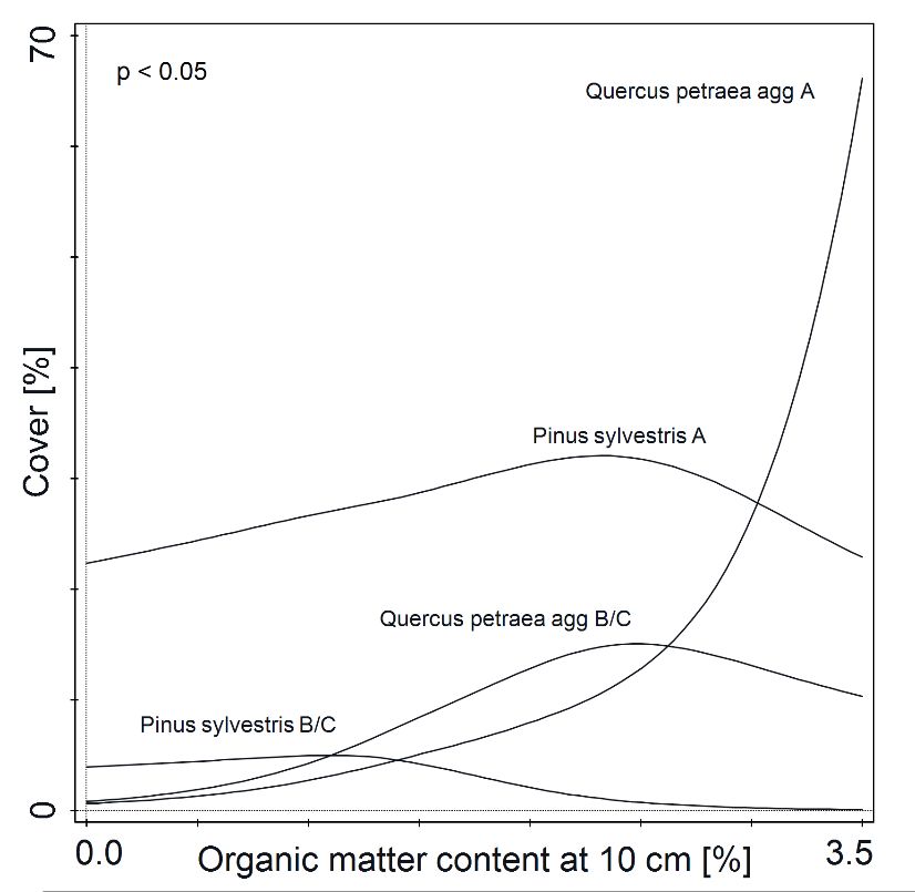
Forests 2022, 13, 198                                                                                            2 of 18

                        tion, leading to the complete disappearance of forest ecosystems, which has occurred in
                        European lowlands since neolithic times [12].
                              One of the main agrotechnical operations influencing the physical, chemical and biolog-
                        ical properties of soil is tillage [13–15]. Agricultural use greatly changes the accumulation
                        of soil organic matter, especially in low-productivity soils [16]. It also accelerates erosion
                        and can lead to soil truncation, degradation and transformation [17,18], thus influencing its
                        differentiation [19].

                        1.2. Influence of Land Use Change on Oligotrophic Forest Dynamics and Forest Conservation in
                        Central Europe
                             Land-use change is considered one of the main drivers of ecosystem dynamics world-
                        wide [20]. Presently, land abandonment is the most frequent reason for landscape change
                        across Europe [21]. This highly dynamic process is driven by a combination of socio–
                        economic, political and environmental factors and influences biodiversity and ecosystem
                        services [22]. It is followed by vegetation succession and seems to be a generally suit-
                        able method of ecosystem restoration, resulting mainly in the formation of secondary
                        forests [23]. In Poland, the agriculture located on low-productivity sandy soils (called
                        Arenosols) was largely abandoned. Nowadays they are predominantly covered by sec-
                        ondary pine forests [24].
                             Ecological succession plays an important role in shaping vegetation structure within
                        both early- [25,26] and late-successional [27,28] ecosystems. The abandonment of tra-
                        ditional forest utilization and changes in anthropogenic disturbance regimes are being
                        observed [29,30]. During the last century, many changes in Central European forest com-
                        munities were observed, including the decrease in oligotrophic pine and oak forests and
                        the expansion of more fertile forest communities, e.g., [27,31–35]. Many of the most vul-
                        nerable forest communities have been protected as Natura 2000 habitats [36]. One of the
                        most threatened forest habitats in lowland Central Europe is the Cladonia-Scots pine forest
                        Cladonio-Pinetum Juraszek 1927 (code: 91T0), which is in decline throughout its entire range,
                        as described in e.g., [33,35,37]. On the other hand, acidophilous oak forest (code: 9190)
                        in Central Europe has expanded [38,39]. While they are protected, many well-preserved
                        patches are found in unprotected sites [40]. Both habitat types occur on sandy soils called
                        Arenosols. Pine forest plantations can be converted into oak forest [41,42], especially on
                        more fertile habitats. The spontaneous ingrowth of oak through forest regeneration is also
                        possible [43], but the possibility of conversion of Cladonia Scots-pine forests to acidophilous
                        oak forests has not been considered in detail. Moreover, these habitat types need different
                        conservation management approaches, cfr. [37,44,45], and for this reason, it is necessary to
                        decide which habitat type to protect—the early- or late-successional one.

                        1.3. Aim
                             A uniquely diverse forest vegetation was identified in Central Poland, on an olig-
                        otrophic sandy site near the village of Kiedrzyn. It consists of abandoned fields, initial,
                        lichen-rich Scots-pine forests, mid-successional moss and dwarf-shrub dominated Scots-
                        pine forests, mixed oak–pine forests and acidophilous sessile oak forests. The aim of this
                        study was to determine the main drivers of differentiation of these forest communities
                        occurring on the same geological substrate. Our specific goal was to assess the impact
                        of past deforestation and soil degradation caused by tillage on the recent diversity of the
                        described forest mosaic, including both regularly and traditionally managed patches.

                        2. Materials and Methods
                        2.1. Study Site
                            The study was carried out within part of a forest complex (ca. 200 ha) located in
                        Central Poland, in the vicinity of Kiedrzyn (20◦ 430 E 51◦ 350 N). The area is covered by
                        deep (up to 20 m) fluvioglacial loose sand deposits. They are partially denudated, with an
                        admixture of loose diluvial sands in local depressions [46]. According to WBR (2015) [47]
Forests 2022, 13, 198 3 of 18
all of the soils within the research area belong to the Arenosol. At the beginning of the
20th century, the central and north-eastern parts of the site were used as arable land [48],
after which most of the fields were gradually abandoned and spontaneously overgrown
or planted with Scots-pine [49–51]. Many phytogenic hillocks are present within parts
of the previously arable area. Such landforms are indicators of soil erosion by wind [52].
The southwestern part of the study site remained afforested during the last century. It is
covered by mixed Scots-pine and sessile oak forests. The mature oak stands, located in the
south-western part of the site, are managed by State Forests. According to information
obtained from local forest administrators and residents, confirmed by our own observations,
they are of old (around 1900 years) coppice origin. The remaining area is private property
covered mainly by naturally regenerated pine forests, with single-tree cutting of Scots pine
being the dominant management practice. This accelerates the natural regeneration of
sessile oak, which encroach into the young secondary pine stands. Nowadays, most of the
area is covered by forest, including two EU Natura 2000 habitat types, acidophilous oak
forests (code: 9190) and Cladonia Scots-pine forests (code: 91T0) together with pine and
mixed oak-pine forest communities. Abandoned fields with psammophilous grasslands
(code: 2330), sparsely overgrown with Scots pine, are also admixed.
2.2. Fieldwork
Fieldwork was conducted during the 2016 growing season. A set of 90 circular sample
plots (400 m2 each) were designated within the study area (Figure 1). One sample per
vegetation type in each forest subdivision was collected within State Forest lands, located
in central parts of subdivisions or habitat patches. On private land the wide diversity of
vegetation and local management types made it impossible to apply a regular sampling
scheme. Forest division boundaries differed significantly from stand borders and habitat
patches. Thus, the main aim there was to sample internally homogeneous patches, differing
in vegetation structure, soil disturbance or management type. Management type was
defined as traditional (natural succession, uneven stand age, single-tree cutting) or regular
(planted, even age stands with regular thinning). Vegetation was sampled using the
Barkman et al. (1964) [53] scale, with cover the measure of species abundance, due to the
preference for pure cover scales in ecological studies [53,54]. The terrain slope angle was
measured with an inclinometer. Within each plot, small soil pits (ca 50 cm deep) were
made, deepened with an auger to a depth of 150 cm, and soil samples were collected at
depths of 10, 30, 70 and 150 cm. In addition, soil profiles were described, soil horizons
distinguished, the presence of plough disturbance determined, and the thickness of the
organic matter horizon measured. The Munsell scale (2009) [55] was additionally used for
color description to confirm the identification of the Bv diagnostic horizon [56], which is
also a Brunic qualifier [47]. The locations of study plots were registered using GPS.
2.3. Laboratory Analysis
Sieving of soil samples was performed using a mesh size of 0.1 mm (fine sand), with the
remainingForests 2022, 13, 198 4 of 18
Forests 2022, 13, x FOR PEER REVIEW 4 of 20
Figure 1. Vegetation types and continuity of forest occurrence in the study area (habitat types: PG—
Figure 1. Vegetation
psammophilous typesCPF—Cladonia-Scots
grassland, and continuity of pineforest occurrence
forest, PF—pine in theOPF—oak–pine
forest, study area (habitat
mixed types:
PG—psammophilous grassland,
forest, AOF—acidophilous CPF—Cladonia-Scots
oak-forest; pine forest, PF—pine
forest continuity: 0—abandoned fields, stillforest, OPF—oak–pine
not afforested in
2014,forest,
mixed 1—afforested in 2014 (but not in
AOF—acidophilous 2001), 2—afforested
oak-forest; since 2001 (but
forest continuity: not in 1982), 3—afforested
0—abandoned fields, still not af-
since 1982 (but not in 1935), 4—afforested since 1935 (but not in 1915), 5—afforested since 1915; R—
forested in 2014, 1—afforested in 2014 (but not in 2001), 2—afforested since 2001 (but not in 1982),
main roads, A—arable land, B—built up areas).
3—afforested since 1982 (but not in 1935), 4—afforested since 1935 (but not in 1915), 5—afforested
since
2.3.1915; R—main
Laboratory roads, A—arable land, B—built up areas).
Analysis
Sieving
2.4. Data of soil samples
Preparation was performed using a mesh size of 0.1 mm (fine sand), with
and Analysis
the remainingForests 2022, 13, 198 5 of 18
Table 1. Cartographic materials used for preparation of forest continuity rank (“zero” value was
assigned if forest was not present in the most recent dataset, with higher ranks assigned when forest
cover was present in earlier datasets, starting from the youngest).
No of Dataset Dataset Scale Actuality Type of Dataset Source of Dataset Forest Continuity Rank Value
1 1:100,000 1915 topographic map [39] 5
2 1:100,000 1935 topographic map [40] 4
3 1:10,000 1982 topographic map [41] 3
4 1:5000 2001 orthophotomap [42] 2
5 1:5000 2014 orthophotomap [42] 1
Forest cover was digitized separately for each dataset. Then the vector forest data were
geoprocessed with the intersect, difference and union GIS tools to produce one map of forest
continuity rank (Figure 1). If forest cover was lacking in the “older” dataset, the rank of
the “younger” value was assigned regardless of the presence of forest on even older maps.
Temporary deforestation was rarely observed in the study site and was not recorded at any of
the studied plots, so it was not taken into the account as a possible additional variable. Thus,
the rank value assigned for each sample plot was the number of datasets with the presence
of forest cover, starting from the most recent one (Table 1). If forest cover was not observed
in the dataset from 2014 (corresponding to recently abandoned fields sparsely covered with
young trees), the “zero” rank value was assigned. The average minimum sampling-point
distance to the closest boundary of the forest continuity patches was 61.60 m and in case of
boundaries derived from georeferenced material 97.72 m respectively.
A high resolution (1 m grid cell with 0.15 m mean height error) Digital Elevation
Model (DEM) was used [51] to calculate the Topographic Position Index (TPI). This index
is defined as the difference between the elevation at a cell and the average elevation of cells
within a predetermined radius [59]. Values greater than zero indicate locations higher than
average (e.g., ridges). Negative values of TPI show lower elevation locations (e.g., valleys).
Values close to zero indicate flat areas and constant slopes. Calculation of TPI at the fine
scale (100 m radius) is considered appropriate for ecological research [59]. TPI can correlate
with the ecological characteristics of the site [60]. Three TPIs were calculated at 25 m, 50 m
and 100 m radii, respectively. Ground water level was calculated on the basis of DEM and a
hydrogeological site map [61]. The assessment of forest continuity and TPI were conducted
with QGIS 3 and SAGA 2 software [62,63].
The maximumForests 2022, 13, 198 6 of 18
2.4.2. Data Analysis
The environmental variables used in this study were of two types: Scale variables,
included pH; conductivity and organic matter content in the soil at a 10 cm depth; organic
horizon thickness, mass percent 0.7). Their simple effects (the variation explained by single variables without covariables)
were lower than for other colinear variables (Table S4 in Supplementary Materials). Non-
scale variables were treated as factors (aggregations of nominal or categorical variables).
Canonical Correspondence Analysis (CCA) was performed. Whole vegetation dataset was
used. A square root vegetation data transformation and downweighting of rare species
were applied. A forward selection procedure was applied to all variables not excluded in
order to identify those that were significant. Selection was stopped at p-value = 0.05 and
the final CCA model was determined (Figure 2). The significance of variable effects and
species–environment relations were checked with a Monte Carlo test (9999 permutations).
The false discovery rate method was used for probability adjustment. Differences in the
values of significant environmental variables between vegetation types were checked by
non-parametric Kruskal–Wallis and Mann–Whitney post-hoc tests (Figure 3). A set of
Generalized Addictive Models (GAM) was calculated, together with response curves for
Pinus sylvestris L. and Quercus petraea (Matt.) Liebl., for soil organic matter content (Figure 4),
according to recommended procedures [65]. CCA ordination and GAM analyses were
performed in CANOCO 5 software [66]. A pairwise correlation analysis of environmental
variables was conducted in PAST 4 software [67].
Vegetation data were classified using Ward’s method, after square root transformation
(Figure S1 in Supplementary Materials). The average cover (Barkman’s Total Cover Value,
TCV) and Phi (Pearson’s ϕ) coefficients (as a measure of species fidelity) were calculated
for each of the groups of plots identified. The significance of species Phi coefficients was
checked with Fisher’s exact test, according to Chytrý et al. (2002) [68]. The groups obtained
were assigned to associations on the basis of cover and fidelity of the dominant and diag-
nostic species according to regional literature [38,69–71]. Ward’s analysis was conducted
using PAST 4 software [67]. The average cover and Phi coefficients, together with Fisher’s
tests, were calculated in JUICE 7 software [72,73]. The EU Natura 2000 habitat types were
identified according to the Interpretation Manual (2013) [36] and regional literature [37,44].
3. Results
The results of CCA indicated significant effects of environmental variables relating to
soil properties, forest continuity and soil disturbance on vegetation composition (Table 3,
Figure 2). The most important variable affecting vegetation composition was thickness of
the soil organic horizon.
For five groups of relevés distinguished in Wards analysis (Figure S1 in Supplementary
Materials), the main diagnostic and dominant species are given in Table 4. The first group
(PG) represents abandoned farmlands, gradually replaced with Scots pine with dominance
by species connected to psammophilous grassland (e.g., Cladonia uncialis (L.) Weber ex F.H.
Wigg. or Polytrichum piliferum Hedw.) in the herb layer. They belong to the Corynephorion
canescentis Klika 1931 alliance and meet the criteria for non-forest EU habitat type no 2330.
The second group (CPF) is the Cladonia-Scots pine forest Cladonio-Pinetum Juraszek 1928,
meeting the criteria of the 91T0 EU habitat type 91T0. It is distinguished by the codom-
inance of lichens on the forest floor and the presence of diagnostic lichen species (e.g.,
Cladonia gracilis (L.) Willd. or C. rangiferina (L.) Weber ex F.H. Wigg.). The third group (PF)
meets the criteria for Vaccinio myrtilli-Pinetum sylvestris Juraszek 1928, a highly common
pine forest type in Central Europe. The fourth group (OPF) reflects mixed oak–pine standsForests 2022, 13, 198 7 of 18
and corresponds to Querco-Pinetum (W. Mat. 1981) J. Mat. 1988. It is a transitional commu-
nity between oak and pine forest types. The fifth group (AOF) represents the Calamagrostio
arundinaceae-Quercetum petraeae Hartm. 1934 Scam. et Pass. 1959 acidophilous oak forest as-
sociation, and thus, the EU Natura 2000 9190 habitat type. It can be distinguished especially
by the dominance of Quercus petraea in the overstory and the presence of Carex pilulifera L.,
Hieracium lachenalii C. C. Gmel., and H. murorum L. in the herb layer as diagnostic species.
Table 3. Environmental variables chosen during the forward selection procedure of CCA (variable
types: general–scale, factor–nominal or categorical, p-values with 9999 Monte Carlo permutations,
false discovery rate method used for p-value adjustment).
Full Name Short Name Variable Type Explains % Contribution % Pseudo-F p-Value p (Adjusted)
organic horizon
org hor general 12.3 25.3 12.3 0.0001 0.0003
thickness [mm]
forest continuity
for con 5 factor 8.4 17.2 9.2 0.0001 0.0003
factor. for con 5
forest continuity
for con 0 factor 6.1 12.5 7.1 0.0003 0.0012
factor. for con 0
forest continuity
for con 1 factor 5.9 12.1 7.4 0.0001 0.0006
factor. for con 1
soil disturbance
soil dist 4 factor 2.6 5.4 3.4 0.0001 0.0005
factor. soil dist 4
organic matter
content in soil at org mat general 1.4 2.8 1.8 0.0113 0.0387
10 cm depth [%]
Table 4. Average percentage cover (Barkman’s TCV) and fidelity (upper index–Phi coefficient given
if Fisher’s test p < 0.05) of species for the groups of plots distinguished by Ward’s method (main
diagnostic and dominant species presented; A—stand, B/C—in undergrowth): PG—psammophilous
grassland, CPF—Cladonia-Scots pine forest, PF—pine forest, OPF—oak–pine mixed forest, AOF—
acidophilous oak forest.
Group of Plots PG CPF PF OPF AOF
Number of samples 13 9 35 26 7
Quercus petraea (Matt.) Liebl. agg A 0.038 0.389 0.057 11.827 42.6 68.714 54.2
Quercus petraea agg B/C 2.481 1.323 2.603 26.154 5.214
Pinus sylvestris L. A 6.692 17.333 46.286 22.8 27.346 22.8 3.857
Juniperus communis L. B/C 2.17 0.578 0.563 1.413 0.943
Betula pendula Roth A 2.669 19.778 53.7 0.271 2.027 1.714
Pinus sylvestris B/C 14.154 26.2 2.157 1.298 0.783 0.006
Convallaria majalis L. 0 0 0 0.008 4.357 78.8
Hieracium lachenalia C. C. Gmel. 0.001 0 0.006 0.008 0.257 78
Calamagrostis arundinacea (L.) Roth 0 0 0 0.008 0.171 57.6
Polytrichastrum formosum (Hedw.) GL Smith 0 0.022 0.007 0.016 0.559 59.9
Siuro-hypnum oedipodium (Mitt.) Ignatov & Huttuman 0.246 0.001 3.167 0.126 0.174 39.6
Hieracium murorum L. 0 0 0 0 0.003 49.2
Carex pilulifera L. 0 0.023 0.017 0.197 14.5 1.457 56.8
Pteridium aquilinum (L.) Kuhn 0 0 0.006 0.497 12 3.957 61.9
Vaccinium myrtillus L. 0.015 0.056 0.661 4.708 16.5 14.571 39.1Forests 2022, 13, 198 8 of 18
Table 4. Cont.
Group of Plots PG CPF PF OPF AOF
Melampyrum pretense L. 0.247 0.512 0.712 1.697 21.4 1.373
Calluna vulgaris (L.) Hull 0 0.022 0 0.37 22.6 0.071
Pleurozium schreberi (Brid.) Mitt 2.24 11.212 55.392 17.2 52.731 7.7
Hieracium pilosella L. 2.169 0.412 0.133 0.021 0
Vaccinium vitis-idaea L. 0 0 0.001 0.354 0.001
Dicranum polysetum Swartz 3.185 8.8 8.581 7.008 0.93
Dicranum scoparium Hedw. 4.493 14.446 6.306 3.134 0.09
Leucobryum glaucum (Hedw.) Ångstr. 0 0.056 0.006 0 0.029
Deschampsia flexuosa (L.) Trin 0 0 0 0.008 0
Cladonia rangiferina (L.) Weber ex F.H.Wigg. 0 8.667 39.9 0.101 0.008 0
Cladonia furcata (Huds.) Schrad. 0.017 0.179 34.4 0.662 0.249 0
Festuca ovina L. 0.463 3.137 28.2 0.051 0.832 3.429
Cladonia gracilis (L.) Willd. 0.586 26.3 3.467 57.3 0.304 0.058 0
Cladonia arbuscula ssp. mitis 19.001 31.1 33.389 54.3 0.831 1.335 0
Cladonia uncialis (L.) Weber ex F.H. Wigg. 4.962 37.9 0.867 50.1 0.132 0.008 0
Cladonia phyllophora Ehrh. ex Hoffm. 0.956 37.6 0.137 34.9 0.108 0 0
Corynephorus canescens (L.) P.Beauv. 1.132 57.9 0.103 31.3 0.129 0 0
Cephaloziella divaricata (Sm.) Schiffn. 0.032 34.4 0 0.001 0 0
Cetraria aculeata (Schreb.) Fr. 0.941 70.5 0 0.006 0 0
Cladonia cervicornis (Ach.) Flot. 0.523 56.4 0 0.001 0 0
Cladonia macilenta Hoffm. 0.804 41.9 0.003 0.02 0.011 0
Polytrichum piliferum Hedw. 6.208 54.7 0.08 0.715 0 0
Stereocaulon condensatum Hoffm. 0.569 61.1 0 0 0 0
Forests 2022, 13, x FOR PEER REVIEW 7 of 20
Figure 2. CCA plot of samples and significant environmental variables (vegetation types: PG—
CCA
Figure psammophilous
2. AOF—acidophilous
forest, plot ofnamessamples andaresignificant
grassland, CPF—Cladonia-Scots pine forest, PF—pine forest, OPF—oak-pine mixed
oak forest; of environmental variables as in Table 3). environmental variables (vegetation types:
PG—psammophilous
Table 3. Environmental variablesgrassland, CPF—Cladonia-Scots
chosen during the forward selection procedure of CCA (variable pine forest, PF—pine forest, OPF—oak-pine
types: general–scale, factor–nominal or categorical, p-values with 9999 Monte Carlo permutations,
mixed forest, AOF—acidophilous oak forest; names of environmental variables are as in Table 3).
false discovery rate method used for p-value adjustment).
Short Variable Contribution
Full Name Explains % Pseudo-F p-Value p (Adjusted)
Name Type %
organic horizon thickness [mm] org hor general 12.3 25.3 12.3 0.0001 0.0003
forest continuity factor. for con 5 for con 5 factor 8.4 17.2 9.2 0.0001 0.0003
forest continuity factor. for con 0 for con 0 factor 6.1 12.5 7.1 0.0003 0.0012
forest continuity factor. for con 1 for con 1 factor 5.9 12.1 7.4 0.0001 0.0006
soil disturbance factor. soil dist 4 soil dist 4 factor 2.6 5.4 3.4 0.0001 0.0005Forests 2022, 13, 198 9 of 18
The organic horizon was thinnest in psammophilous grasslands (PG). Medium values
of this variable were a feature of Cladonia-Scots pine forests (CPF) and acidophilous oak
forests (AOF), and the highest values occurred within pine forests (PF) and oak–pine forests
(OPF) (Figure 3A). All of the habitats but AOF had lower forest continuity (Figure 3B). Addi-
tionally, some differed between themselves. Early successional habitats (PG, CPF, and PF)
were characterized by higher soil disturbance ranks than late-successional ones (OPF and
AOF), however AOF suffered the least soil disturbance (Figure 3C). Soil organic matter
content was lower in PG, CPF, and PF habitat types. Higher values of soil organic matter
were associated with OPF and AOF communities (Figure 3D).
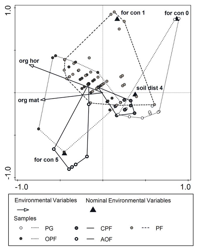
Models
Forests 2022, of the
13, x FOR PEER response of Pinus sylvestris L. and Quercus petraea (Matt.) Liebl.8 to
REVIEW of 20percent
organic matter content in soil were significant (p < 0.05) (Figure 4). Medium values of
organic matter in soil were connected with a higher abundance of Scots pine. Higher values
organic matter content in soil at
org mat general 1.4 2.8 1.8 0.0113 0.0387
were 10 associated
cm depth [%]with a greater abundance of sessile oak. Both species were less abundant
in soils with the lowest organic matter content.
Figure 3. Variation in main
Figure environmental variables
3. Variation in main between
environmental vegetation
variables betweentypes (PG—psammophilous
vegetation types (PG—
psammophilous grasslands on abandoned fields 2330, CPF—Cladonia-pine forest 91T0, PF—pine
grasslands on abandoned forest, OPF—oak–pine mixed forest, AOF—acidophilous oak forest 9190): (A) organic OPF—oak–
fields 2330, CPF—Cladonia-pine forest 91T0, PF—pine forest, layer
thickness, (B) forest continuity
pine mixed forest, AOF—acidophilous oakrank, (C) soil
forest disturbance
9190): (A)rank, (D) organic
organic layermatter content in soil(B)
thickness, at forest
10 cm, (Kruskal–Wallis and Mann–Whitney post hoc, Holm–Bonferroni sequential correction used
continuity rank, (C) soilfordisturbance rank,
p-value adjustment, (D) organic
lowercase matter content
letters—homogenous groups atin soil= at
alpha 10 cm, (Kruskal–Wallis
0.05).
and Mann–Whitney post hoc, Holm–Bonferroni sequential correction used for p-value adjustment,
lowercase letters—homogenous groups at alpha = 0.05).Forests
Forests2022,
2022, 13,
13, x198
FOR PEER REVIEW 910ofof20
18
Figure 4. The
Figure Therelationship
relationshipbetween
between soilsoil
organic matter
organic content
matter and percentage
content Pinusof
cover ofcover
and percentage sylvestris
Pinus
sylvestris andpetraea
and Quercus Quercusaggpetraea
in treeagg in tree
stands (A)stands (A) and undergrowth
and undergrowth (B/C) (Pinus(B/C) R2 = 0.034,
(PinusAsylvestris:
sylvestris: AR 2 =
B/C
0.034,
R2 = 0.184;
2 = 0.184;petraea
B/C RQuercus Quercus petraea
agg: A R2agg: A R B/C
= 0.269,
2 = 0.269,
R2 =B/C R =N0.194;
2
0.194; N =all90,
= 90, in in all
cases pForests 2022, 13, 198 11 of 18
years after the cessation of tillage, e.g., [75]. Then, the first shrub and tree species appear
and gradually change the non-forest communities into oligotrophic pine forests, with a
forest floor dominated by lichens or mosses. This stage can last ca. 40–70 years [25,75].
The Cladonia-rich pine forests are nowadays considered transitional communities, and only
persist in the lichen-abundant form for between ca. 22–36 years [32]. The successional sere
is usually finished at the point of mesic pine forest, which is often considered a climax
forest formation within such sites, developing after ca. 60–70 years of succession [25,75,76].
On the other hand, spontaneous oak encroachment into pine stands on sandy soils has
been observed [43,77,78] and acidophilous oak forest has become more common in the
Central European landscape [38,39]. This could potentially prolong the possible trajectory
of succession on an oligotrophic, sandy substrate. It is highly probable that the documented
vegetation diversity belongs to the same sere. It would be a much longer sere, compared to
others reported in research on forest succession in Europe. They tend to be much shorter
and usually include one or two forest communities, often compared with some pre-forest
vegetation, i.e., [23,26,39,76].
4.3. Historic Soil Disturbance by Tillage Explains the Present Diversity of Vegetation
Brunic Arenosols (commonly called rusty soils in Poland) are formed from sands and
can be distinguished by a thick Bv (sideric) horizon of diagnostic value [79]. Forests are
known for their soil-protecting role [80], which is manifested in this study by the lowest
level of soil disturbance in mature oak stands (AOF), characterized by high forest continuity.
Agricultural soil disturbance is caused mainly by tillage. Plowing results in erosion by
exposure of the soil surface to wind and water, e.g., [17,18,64,80]. The results of this process
were observed within the study site. They were manifested firstly by the presence of a
plough layer and secondly through increasing denudation of the soil Bv horizon. In such
cases, Brunic Arenosols lose their diagnostic Bv horizon and are named Haplic Arenosols
(typical) or Protic Arenosols (initial) in the case of close to complete soil profile destruction.
Soil truncation of Brunic Arenosols can easily reach 40–50 cm [18]. Such a high level of
denudation is probable within the study site. Denudation was also indirectly identified in
the field by the presence of common juniper (Juniperus communis L.) on phytogenic hillocks,
often observed in the vicinity of plots characterized by the highest levels of soil degradation.
This type of formation results from wind erosion [52].
Time since agricultural land abandonment is an important factor influencing forest
species composition [81]. In this study, the AOF (and partially OPF) vegetation were
characterized by higher forest continuity. Lower continuity was a feature of PG and pine
forests. The significance of this time-related variable in the final CCA model indicates the
succession process occurring within the study site. The regeneration of forest is slower
within more oligotrophic habitats [25,81]. This may be the reason for CPF tendency to
slower regeneration than PF.
Agricultural use of sandy forest soils leads to decreased organic carbon and soil
organic matter [15,82]. Moreover, soil organic matter accumulation is a good predictor of
successional changes [83]. One of the characteristic features of early successional habitats,
such as psammophilous grasslands and Cladonia-Scots pine forest, is low organic matter
content in soil [8,84]. Pine forests are characterized by only slightly higher organic matter
content [8], with the highest soil organic matter in oak forests [9], a result confirmed in
this study. Despite this, a high negative correlation between soil disturbance rank and
organic matter content suggests that the level of initial habitat impoverishment by tillage
can be of the same importance as the increase in organic matter content observed during
succession [83]. Soil fertility is an important driver of community assembly during forest
succession [85]. Thus succession within initially more organic matter-rich sandy soils is
faster than within soils characterized by lower organic matter content [25]. Such a process
likely occurred in this study. This can also explain the higher cover of oak in undergrowth
within more organic matter-rich plots, in spite of the fact, that colonization by oak could
have begun together with pine during the transition from the non-forest habitats [86].Forests 2022, 13, 198 12 of 18
Soil pH had no explanatory power in the CCA model and soil conductivity was
colinear. However, their correlations with organic matter content are also interpretable.
The pH of the upper soil horizons of arable fields is higher than that of forest stands [15],
most likely because of the high acidity of pine needles. In spite of its importance for
nutrients cycling in topsoil [87], the decay of coniferous litterfall can decrease soil pH under
trees [88] and accelerate podzolization process [89]. In the present study, the increase in soil
conductivity was changing with vegetation. This was most likely connected with rising
concentrations of H+ ions caused by the increasing presence of organic acids in oligotrophic
and humus-enriched soils, as soil conductivity was positively correlated with organic
matter concentration at 10 cm and negatively with soil pH at 10 cm. Such a relationship
can be observed within early successional habitats affected by the accumulation of strongly
acidic litter [90]. However, the organic matter concentration at 10 cm had better explanatory
power in CCA. This supports its use as a variable connected with successional changes,
as proposed by Walker et al. [83].
Litter accumulation influences species composition [90]. A low amount of litter is
particularly suitable for Cladonia species and can be observed in psammophilous grasslands
and Cladonia-rich pine forests [84,91]. A thicker layer of organic matter is characteristic
of other pine and acidophilous oak forests [8,9]. The growing thickness of the organic
horizon is connected to coniferous litter accumulation over time. The disintegration of pine
needle litter is much slower than oak leaves [92] and results in thinner layers of organic
matter under oak trees. This explains the finding of slightly lower values of organic horizon
thickness observed in AOF.
Previous tillage-connected soil disturbance resulted in soil truncation and degradation
of soil profiles within the study site. This was demonstrated by the decrease in organic
matter content (but also by raised pH and decreased conductivity of soils). The aban-
donment of agricultural cultivation enabled secondary succession. However, it occurred
especially on close to initial post-agricultural soil conditions. This favored the develop-
ment of Cladonia-rich non-forest and then forest habitat types, both protected as Natura
2000 habitats (2330, 91T0). Mid-successional communities were of lower conservation
value. A gradual replacement of pine by oak is observed in the undergrowth and increas-
ingly in tree stands on the research site. Such changes were also documented in other
studies, e.g., [26,78], but the process was usually less well advanced. The spontaneous
replacement of pine by oak in undisturbed habitats tends to be slow because both species
are long-lived [78]. The complete replacement of pine by oak in the study site was observed
in the older oak stands with undisturbed soil. It was also evident in some post-agricultural
plots. We think that this process was enhanced by traditional management of private
forest land, where there was better establishment of oak within patches with less degraded
soils, however management type did not contribute to the final CCA model. Traditional
management is still practiced in some private forests in Poland, usually involving the
gradual harvesting of older pine, leading to a reduction in light concurrency [93]. This
enhances oak development [94]. Young oak in the understory tend to be omitted during
harvesting and gradually reach the tree layer. After pine replacement by oak, vegetation
reaches the late-successional stage acidophilous oak-forest, the other Natura 2000 habitat
type (9190). The results indicate that the temporary coexistence of four unique types of
forest communities (including two Natura 2000 forest habitat types) is possible within one
homogenous geological substrate.
This study provides information that may be used to determine the potential natural
vegetation (PNV) of the study site. The concept was introduced by Tüxen in 1956 [95]
and, despite some misunderstanding and thus criticism, it has been used widely as
a valuable decision-support tool for land management and ecological restoration [96].
The interpretation by Somodi et al. (2021) [97] of Tüxen’s original PNV definition (as well
as subsequent and related definitions) was used to interpret the results of this study. As the
concept leaves some discretion in its interpretation, a rough and clear division into pine
and oak forest was adopted. The PNV is focused on the actual habitat conditions of theForests 2022, 13, 198 13 of 18
analyzed areas and incorporates anthropogenic impacts on soil. Nowadays, impoverished
soils are mainly regenerated with coniferous trees. The abundance of oak was much lower
within habitats characterized by low soil organic matter content. Thus the current PNV
of the study site consists of both pine (in habitats with soil-disturbance) and oak forests
(in less impoverished soils or undisturbed habitats). The potentially restorable vegetation
(PRV), in the sense of Somodi et al. (2021) [97], corresponds with the reconstructed nat-
ural vegetation as conceptualized by Moravec (1998) [98], in which the entire study site
would be acidophilous oak forest. It can be concluded, that due to human impact on soil,
the actual PNV differs from PRV.
4.4. Implications for Forest Management and Conservation
4.4.1. Implications for Nature Conservation
Agricultural deforestation was once a common practice in Eurasia [12]. Nowadays,
land abandonment is the most frequent driver of landscape change across Europe [21].
In Poland, the share of post-agricultural lands in State Forests is at least 22.1% [24]. Land
abandonment leads not only to ecological succession, but also to changes in forest dis-
turbance [30]. As a result, many human disturbance-related ecosystems, including some
early successional and disturbance-related forests, became increasingly threatened. Their
conservation requires anthropogenic disturbance, e.g., [91,99–102], even drastic soil distur-
bance in the case of initial, psammophilous habitats [84,103]. Importantly, in this study,
the occurrence of Cladonia-Scots pine forest was dependent on prior agricultural use and
soil impoverishment. As a transitional and short-lived forest type [32,33,37], it requires
active conservation in order to persist while maintaining its inherent biodiversity. Litter-
raking and single-tree cutting are usually thought to be potential traditional forms of
Cladonia-Scots pine forest management [37,91,104]. Our results suggest that strong soil
disturbance is a possible method of maintaining this habitat-type, however it is difficult
to implement in afforested landscapes and in light of general trends in nature protection
strategies within European Union [105]. Moreover, secondary succession within the close-
to-initial sandy conditions is a slow process, e.g., [25,26,75]. Due to this, ploughing cannot
be used for short-term habitat conservation. Litter-raking and deadwood removal appear
to be more appropriate strategies, as thinner litter layer is characteristic of Cladonia-rich
forests [45,91]. Additionally, litter-raking is known to decrease soil fertility [106,107]. It is
worth mentioning, that Cladonia-rich pine forest communities are vanishing, not only from
the Central European landscape, but also in Scandinavia, where they are an important food
source for reindeer, i.e., [108,109].
In contrast, acidophilous oak forest can function successfully both with and without
human assistance [40]. It is a late-successional community on an oligotrophic, sandy sub-
strate [44]. This habitat type tends to be expanding in Central Europe [38,39]. Both passive
protection and sustainable forest management can ensure its effective conservation [44].
The potential co-occurrence of two completely different, legally protected EU forest
Natura 2000 habitat types has implications for conservation planning. In some cases,
this may result in the need to reassess management decisions, since planning to protect one
type may lead to the exclusion of the other.
4.4.2. Implications to Forest Management
Conservation of Cladonia-Scots pine forests faces difficulties due to insufficient knowl-
edge, and the rapid reduction in the area covered by this community. Overall, well-proven
conservation methods are lacking, but some traditional procedures that reduce canopy
closure are likely appropriate. The introduction of any understory is discouraged [37].
Large-scale clearcutting is also sometimes proposed [104]. The results of this study favor
increased soil disturbance as a possible long-term habitat management tool. However,
such a practice is becoming less acceptable in modern forestry, which is instead focused on
the replacement of pine stands by mixed pine–oak and pure oak stands [41,110]. Given thatForests 2022, 13, 198 14 of 18
Cladonia-Scots pine forest can occur both on Brunic Arenosols and Haplic Arenosols [8], litter
raking seems a possible method to promote Cladonia-Scots pine forest habitat conservation.
Due to their low agricultural suitability, Brunic Arenosols were mostly abandoned and
then afforested in the 20th century. Nowadays, they occupy 65.8% of all post-agricultural
lands in Polish State Forests, and are predominantly covered by pine forests [24]. Intact
Brunic Arenosols are suitable for forestry and enable the cultivation of broadleaved forests,
e.g., pedunculate and sessile oaks [111]. When these soils are degraded by podzolization,
they are more appropriate for Scots pine [112]. In our study, plots with slightly degraded
Brunic Arenosols were intensively colonized by oak, whereas sites with a strongly de-
nudated soil profile were dominated by pine. Thus, we conclude that slightly degraded
post-agricultural sandy soils can support oak forest. Sites with intermediate levels of
disturbance tend to be more suitable for pine plantations, and forest patches characterized
by the highest levels of soil profile degradation should be the focus of Cladonia-Scots pine
forest conservation.
5. Conclusions
• Past soil disturbance resulting from tillage is the main factor enhancing the diversity
of forest communities in the oligotrophic fluvioglacial site.
• The presence of two protected forest EU Natura 2000 habitat types, which need differ-
ent management methods, may require choosing, whether to protect transitional and
anthropogenic Cladonia-Scots pine forest (code 91T0) or late-successional acidophilous
oak forest (code: 9190). Management decisions will be more concerned with the fate
of lichen-rich pine forests.
• It may be necessary to reassess management plans and conservation decisions when
considering forests on oligotrophic-sandy substrates.
• Post-agricultural Brunic Arenosols that are lightly degraded appear to promote oak
establishment, while medium soil disturbance favors pine plantations.
• Near complete soil-profile denudation can be used as an indicator of potential sites for
Cladonia-Scots pine forest conservation.
• The potential natural vegetation of the study site differs from potentially restorable
vegetation: the PNV of pine forest is still pine forests, the PNV of oak–pine forest and
acidophilous oak forest is acidophilous oak forest, and the PRV of the entire study site
is acidophilous oak forest.
Supplementary Materials: The following supporting information can be downloaded at: https:
//www.mdpi.com/article/10.3390/f13020198/s1, Table S1: vegetation data; Table S2: environmental
data; Table S3: Spearman’s rank correlations of the explanatory variables; Table S4: environmental
variables used in forward selection procedure of CCA; Figure S1: dendrogram of Ward’s analysis.
Author Contributions: Conceptualization P.T.Z. and A.O.; methodology P.T.Z.; formal analysis P.T.Z.,
investigation, P.T.Z., W.C. and K.M.; writing—original draft preparation, P.T.Z.; writing—review and
editing, P.T.Z., A.O., W.C. and K.M.; visualization P.T.Z.; funding acquisition P.T.Z. All authors have
read and agreed to the published version of the manuscript.
Funding: This research was funded by the Institute of Forest Sciences, Warsaw University of Life
Sciences within grant no. 505-10-031100-P00571-99.
Institutional Review Board Statement: Not applicable.
Informed Consent Statement: Not applicable.
Data Availability Statement: The supporting data are stored in the Supplementary Materials.
Acknowledgments: We would like to thank Artur P˛edziwiatr from the Department of Soil Science,
WULS-SGGW, for his kind help with the Munsell scale.
Conflicts of Interest: The authors declare no conflict of interest. The funders had no role in the design
of the study; in the collection, analyses, or interpretation of data; in the writing of the manuscript,
or in the decision to publish the results.Forests 2022, 13, 198 15 of 18
References
1. Peterken, G.F. Natural Woodland, Ecology and Conservation in Northern Temperate Regions; Cambridge University Press: Cambridge, UK, 1996.
2. Shorohova, E.; Kuuluvainen, T.; Kangur, A.; Jõgiste, K. Natural stand structures, disturbance regimes and successional dynamics
in the Eurasian boreal forests: A review with special reference to Rusian studies. Ann. For. Sci. 2009, 66, 201. [CrossRef]
3. Härdtle, W.; von Oheimb, G.; Westphal, C. Relationships between the vegetation and soil conditions in beech and beech-oak
forests of northern Germany. Plant Ecol. 2005, 177, 113–124. [CrossRef]
4. Neri, A.V.; Schaefer, C.E.G.R.; Silva, A.F.; Souza, A.L.; Ferreira-Junior, W.G.; Meira-Neto, J.A.A. The influence of soil conditions
on the floristic composition and community structure of an area of Brazilian Cerrado vegetation. Edinb. J. Bot. 2012, 69, 1–27.
[CrossRef]
5. Zhang, C.; Li, X.; Chen, L.; Xie, G.; Liu, C.; Pei, S. Effects of Topographical and Edaphic Factors on Tree Community Structure and
Diversity of Subtropical Mountain Forests in the Lower Lancang River Basin. Forests 2016, 7, 222. [CrossRef]
6. Higgins, M.A.; Roukolainen, K.; Tuomisto, H.; Llerena, N.; Cardenas, G.; Phillips, O.L.; Vásquez, R.; Räsänen, M. Geological
control of floristic composition in Amazonian forests. J. Biogeogr. 2011, 38, 2136–2149. [CrossRef] [PubMed]
7. Reczyńska, K.; Pech, P.; Świerkosz, K. Phytosociological Analysis of Natural and Artificial Pine Forests of the Class Vaccinio-
Piceetea Br.-Bl. in Br.-Bl. et al. 1939 in the Sudetes and Their Foreland (Bohemian Massif, Central Europe). Forests 2021, 12, 98.
[CrossRef]
8. Zwydak, M.; Lasota, J.; Brożek, S.; Wanic, T. Różnorodność gleb zespołów borów sosnowych. Rocz. Glebozn. 2011, 62, 39–53.
9. Lasota, J. Siedliskowo-florystyczna analiza środkowoeuropejskiego acydofilnego lasu d˛ebowego (Calamagrostio arundinaceae-
Quercetum petraeae [Hatm. 1934], Scam.et Pass. 1959). Zesz. Nauk. UR im. Hugona Kołłataja ˛ w Krakowie 2013, 393, 5–143.
10. Sewerniak, P. Differences in early dynamics and effects of slope aspect between naturally regenerated and planted Pinus sylvestris
woodland on inland dunes in Poland. iForest 2016, 9, 875–882. [CrossRef]
11. Danneyrolles, V.; Dupuis, S.; Fortin, G.; Leroyer, M.; de Römer, A.; Terrail, R.; Vellend, M.; Boucher, Y.; Laflamme, J.; Bergeron, Y.;
et al. Stronger influence of anthropogenic disturbance than climate change on century-scale compositional changes in northern
forests. Nat. Commun. 2019, 10, 1265. [CrossRef]
12. Kaplan, J.O.; Krumhardt, K.M.; Zimmermann, N. The prehistoric and preindustrial deforestation of Europe. Quat. Sci. Rev. 2009,
28, 3016–3034. [CrossRef]
13. Halpern, M.T.; Whalen, J.K.; Madramootoo, C.A. Long-term tillage and residue management influences soil C and N dynamics.
Soil Sci. Soc. Am. J. 2010, 74, 1211–1217. [CrossRef]
14. Van Eerd, L.L.; Congreves, K.A.; Hayes, A.; Verhallen, A.; Hooker, D.C. Long-term tillage and croprotation effects on soil quality,
organic carbon, and total nitrogen. Can. J. Soil Sci. 2014, 94, 303–315. [CrossRef]
15. Kobierski, M.; Cieścińska, B.; Cieściński, J.; Kondrakiewicz-Maciejewska, K. Effect of Soil Management Practices on the Mineral-
ization of Organic Matter and Quality of Sandy Soils. J. Ecol. Eng. 2020, 21, 217–223. [CrossRef]
16. Kazlauskaite-Jadzevice, A.; Tripolskaja, L.; Volungevicius, J.; Baksiene, E. Impact of land use change on organic carbon sequestra-
tion in Arenosol. Agric. Food Sci. 2019, 28, 9–17. [CrossRef]
17. Van Oost, K.; Govers, G.; de Alba, S.; Quine, T.A. Tillage erosion: A review of controlling factors and implications for soil quality.
PPG Earth Environ. 2006, 30, 443–466. [CrossRef]
18. Świtoniak, M. Use of soil profile truncation to estimate influence of accelerated erosion on soil cover transformation in young
morainic landscapes, North-Eastern Poland. Catena 2014, 116, 173–184. [CrossRef]
19. Sewerniak, P.; Jankowski, M.; Dabrowski,
˛ M. Effect of topography and deforestation on regular variation of soils on inland dunes
in the Toruń Basin (N Poland). Catena 2017, 149, 318–330. [CrossRef]
20. Winkler, K.; Fuchs, R.; Rounsevell, M.; Herold, M. Global land use changes are four times greater than previously estimated.
Nat. Commun. 2021, 12, 2501. [CrossRef]
21. Plieninger, T.; Draux, H.; Fagerholm, N.; Bieling, C.; Bürgi, M.; Kizos, T.; Kuemmerle, T.; Primdahl, J.; Verburg, P.H. The driving
forces of landscape change in Europe: A systematic review of the evidence. Land Use policy 2016, 57, 204–214. [CrossRef]
22. Ustaoglu, E.; Collier, M.J. Farmland abandonment in Europe: An overview of drivers, consequences, and assessment of the
sustainability implications. Environ. Rev. 2018, 26, 396–416. [CrossRef]
23. Prah, K.; Řehounková, K.; Lencová, K.; Jírova, A.; Konvalinková, P.; Mudrák, O.; Študent, V.; Vaněček, Z.; Tichý, L.; Petřík, P.; et al.
Vegetation succession in restoration of disturbed sites in Central Europe: The direction of succession and species richness across
19 seres. Appl. Veg. Sci. 2014, 17, 193–200. [CrossRef]
24. Sewerniak, P. Survey of some attributes of post-agricultural lands in Polish State Forests. Ecol. Quest. 2015, 22, 9–16. [CrossRef]
25. Rahmonov, O. Relacje Mi˛edzy Roślinnościa˛ i Gleba˛ w Inicjalnej Fazie Sukcesji na Obszarach Piaszczystych; Prace Naukowe Uniwersytetu
Ślaskiego
˛ w Katowicach 2506; Wydawnictwo Uniwersytetu Ślaskiego: ˛ Katowice, Poland, 2007.
26. Prah, K.; Ujházy, K.; Knopp, V.; Fanta, J. Two centuries of forest succession, and 30 years of vegetation changes in permanent
plots in an inland sand dune area, The Netherlands. PLoS ONE 2021, 16, e0250003. [CrossRef]
27. Brzeziecki, B.; Pommerening, A.; Miścicki, S.; Drozdowski, S.; Żybura, H. A Common Lack of Demographic Equilibrium among
Tree Species in Białowieża National Park (NE Poland): Evidence from Long-Term Plots. J. Veg. Sci. 2016, 27, 460–469. [CrossRef]
28. Brzeziecki, B.; Woods, K.; Bolibok, L.; Zajaczkowski,
˛ J.; Drozdowski, S.; Bielak, K.; Żybura, H. Over 80 years without major
disturbance, late-succesional Białowieża woodlands exhibit complex dynamism, with coherent compositional shifts towards true
old-growth conditions. J. Ecol. 2020, 108, 1138–1154. [CrossRef]Forests 2022, 13, 198 16 of 18
29. Benayas, J.M.; Martins, A.; Nicolau, J.M.; Schulz, J.J. Abandomnent of agricultural land: An overview of drivers and consequences.
CAB Rev. Perspect. Agric. Vet. Sci. Nutr. Nat. Resour. 2007, 2, 057. [CrossRef]
30. Mantero, G.; Morresi, D.; Marzano, R.; Motta, R.; Mladenoff, D.J.; Garbarino, M. The influence of land abandonment on forest
disturbance regimes: A global review. Landsc. Ecol. 2020, 35, 2723–2744. [CrossRef]
31. Jakubowska-Gabara, J. Decline of Potentillo albae-Quercetum Libb. 1933 Phytocoenoses in Poland. Vegetatio 1996, 124, 45–59.
Available online: http://www.jstor.org/stable/20048679 (accessed on 30 November 2021).
32. Zaniewski, P.T.; Potoczny, B.; Matuszkiewicz, J.M. Modelowanie trwałości boru chrobotkowego Cladonio-Pinetum Juraszek
1927 na terenie Parku Narodowego “Bory Tucholskie” z wykorzystaniem metody powtórzonej chronosekwencji. Sylwan 2016,
160, 397–406. [CrossRef]
33. Stefańska-Krzaczek, E.; Fałtynowicz, W.; Szypuła, B.; Kacki,˛ Z. Diversity loss of lichen pine forests in Poland. Eur. J. For. Res. 2018,
137, 419–431. [CrossRef]
34. Ciurzycki, W.; Brzeziecki, B.; Zaniewski, P.T.; Keczyński, A. Zmiany leśnych zbiorowisk roślinnych w latach 1959–2016 na stałej
powierzchni badawczej w oddziale 319 Białowieskiego Parku Narodowego. Sylwan 2018, 162, 907–914. [CrossRef]
35. Reinecke, J.; Klemm, G.; Heinken, T. Vegetation change and homogenization of species composition in temperate nutrient
deficient Scots pine forests after 45 yr. J. Veg. Sci. 2014, 25, 113–121. [CrossRef]
36. Interpretation Manual of European Union Habitats—EUR28. European Comission DG Environment, Nature ENV 2013,
B.3. Available online: https://ec.europa.eu/environment/nature/legislation/habitatsdirective/docs/Int_Manual_EU28.pdf
(accessed on 30 November 2021).
37. Danielewicz, W.; Pawlaczyk, P. Śródladowy
˛ bór chrobotkowy. In Poradniki Ochrony Siedlisk i Gatunków Natura 2000—Podr˛ecznik
Metodyczny, Tom 5, Lasy i Bory; Herbich, J., Ed.; Ministerstwo Środowiska: Warszawa, Poland, 2004; pp. 289–296.
38. Kasprowicz, M. Acidophilous oak forests of the Wielkopolska region (West Poland) against the background of Central Europe.
Biodivers. Res. Conserv. 2010, 20, 1. [CrossRef]
39. Zaniewski, P.T.; Ciurzycki, W.; Zaniewska, E. The proposal of a new provisional border of range of the acidophilous oak forest
Calamagrostio arundinaceae-Quercetum petraeae Hartm. 1934 Scam. et Pass. 1959 in central Poland. Folia For. Pol. Ser. A For. 2021,
63, 243–259. [CrossRef]
40. Reczyńska, K.; Świerkosz, K. Does Protection Really Matter? A Case Study from Central European Oak Forests. Diversity 2020, 12, 6.
[CrossRef]
41. Zerbe, S. Restoration of natural broad-leaved woodland in Central Europe on sites with coniferous forest plantations.
For. Ecol. Manag. 2002, 167, 27–42. [CrossRef]
42. Vrška, T.; Ponikelský, J.; Pavlicová, P.; Janík, D.; Adam, D. Twenty years of conversion: From Scots pine plantations to oak
dominated multifunctional forests. iForest 2016, 10, 75–82. [CrossRef]
43. Goris, R.; Kint, V.; Hanecca, K.; Geudens, G.; Beeckman, H.; Verheyen, K. Long-term dynamics in a planted conifer forest with
spontaneous ingrowth of broad-leaved trees. Appl. Veg. Sci. 2007, 10, 219–228. [CrossRef]
44. Pawlaczyk, P. Kwaśne dabrowy
˛ (Quercetea robori-petraeae). In Monitoring Siedlisk Przyrodniczych. Przewodnik Metodyczny. Cz. III;
Mróz, W., Ed.; GIOŚ: Warszawa, Poland, 2012; pp. 272–291.
45. Fischer, A.; Michler, B.; Fischer, H.S.; Brunner, G.; Hösch, S.; Schultes, A.; Titze, P. Flechtenreiche Kiefernwälder in Bayern:
Entwicklung und Zukunft. Tuexenia 2015, 35, 9–29. [CrossRef]
46. Skompski, S.; Makowska, A.; Jakubowicz, B. Objaśnienia do Szczegółowej Mapy Geologicznej Polski 1:50,000 Nowe Miasto nad Pilica˛
(669); PIG PIB: Warszawa, Poland, 2013.
47. WBR 2015. IUSS Working Group WRB. World Reference Base for Soil Resources 2014, Update 2015 International Soil Classification System
for Naming Soils and Creating Legends for Soil Maps; World Soil Resources Reports No. 106; FAO: Rome, Italy, 2015.
48. Karte des Westlichen Russlands. G35. Nowe Miasto a/Pilica. 1:100,000; Königlich Preußische Landesaufnahme: Berlin, Germany, 1915.
49. WIG. PAS 42 SŁUP 31 Nowe Miasto nad Pilica.˛ 1:100,000; Wojskowy Instytut Geograficzny: Warszawa, Poland, 1937.
50. GUGIK. Arkusz Tomczyce 124.311, Mapa Topograficzna Polski w Układzie Współrz˛ednych 1965 Skala 1:10,000; Główny Urzad ˛ Geodezji
i Kartografii: Warszawa, Poland, 1982.
51. GEOPORTAL 2021, Ortophotomap of Poland, Scale 1:5000, Sheets No M-34-18-A-b-4-3, M-34-18-A-b-4-4 Actuality 2001. 2014.
Available online: https://mapy.geoportal.gov.pl/imap/Imgp_2.html?gpmap=gp0 (accessed on 10 October 2021).
52. Rahmonov, O.; Snytko, V.A.; Szczypek, T. Phytogenic hillocks as an effect of indirect human activity. Z. Geomorphol. N. F. 2009,
53, 359–370. [CrossRef]
53. Barkman, J.J.; Doing, H.; Segal, S. Kritische Bemerkungenund Vorschläge zur quantitativen Vegetationsanalyse. Acta Bot. Neerl.
1964, 13, 394–419. [CrossRef]
54. Dengler, J.; Chytrý, M.; Ewald, J. Phytosociology. In General Ecology. Vol. 4 of Encyclopedia of Ecology; Jørgensen, S.E., Fath, B.D.,
Eds.; Elsevier: Oxford, UK, 2008; pp. 2769–2779. [CrossRef]
55. Munsell Soil Colour Charts, Munsell Soil Colour Charts: With Genuine Munsell Color Chips; 2009 Year Revised, 2017 Production;
Munsell Color: Grand Rapids, MI, USA, 2009.
56. Kabała, C.; Charzyński, P.; Chodorowski, J.; Drewnik, M.; Glina, B.; Greinert, A.; Hulisz, P.; Jakowski, M.; Jonczak, J.; Łabaz, B.;
et al. Polish Soil Classification, 6th edition—Principles, classification scheme and correlations. Soil Sci. Ann. 2019, 70, 71–97.
[CrossRef]You can also read