Physical conditions and chemical abundances in photoionized nebulae from optical spectra
←
→
Page content transcription
If your browser does not render page correctly, please read the page content below
Physical conditions and chemical abundances in
                                               photoionized nebulae from optical spectra

                                               Jorge García-Rojas
arXiv:2001.03388v1 [astro-ph.SR] 10 Jan 2020

                                               Abstract This chapter presents a review on the latest advances in the computation of
                                               physical conditions and chemical abundances of elements present in photoionized
                                               gas (H ii regions and planetary nebulae). The arrival of highly sensitive spectrographs
                                               attached to large telescopes and the development of more sophisticated and detailed
                                               atomic data calculations and ionization correction factors have helped to raise the
                                               number of ionic species studied in photoionized nebulae in the last years, as well
                                               as to reduce the uncertainties in the computed abundances. Special attention will be
                                               given to the detection of very faint lines such as heavy-element recombination lines
                                               of C, N and O in H ii regions and planetary nebulae, and collisionally excited lines
                                               of neutron-capture elements (Z>30) in planetary nebulae.

                                               1 A very brief introduction on emission line spectra of
                                                 photoionized nebulae

                                               Photoionized nebulae (i. e. H ii regions and planetary nebulae) are among the most
                                               “photogenic” objects in the sky. Given their relatively high surface-brightness they
                                               are easily accessible, even for non-professional telescopes. This allowed earliest
                                               visual spectroscopic observations by William Huggins and William A. Miller ([1])
                                               who obtained the first spectrum of a planetary nebula (The Cat’s Eye Nebula), where
                                               they detected a bright emission line coming from a mysterious element that Margaret
                                               L. Huggins ([2]) called “nebulium”. Several decades later, Ira S. Bowen ([3]) showed
                                               that this emission was produced by doubly ionized oxygen (O2+ ) at extremely low
                                               densities. An historical review on the early steps of the study of the physics of gaseous

                                               Jorge García-Rojas
                                               Instituto de Astrofísica de Canarias, E-38200, La Laguna, Tenerife, Spain. Universidad de La
                                               Laguna. Depart. de Astrofísica, E-38206, La Laguna, Tenerife, Spain e-mail: jogarcia@iac.es

                                                                                                                                         1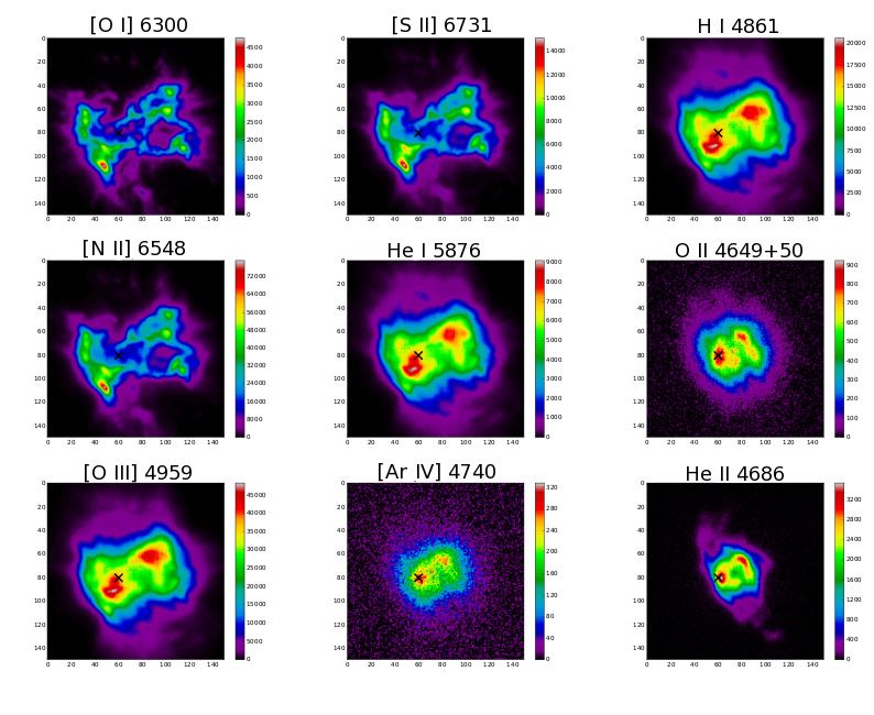
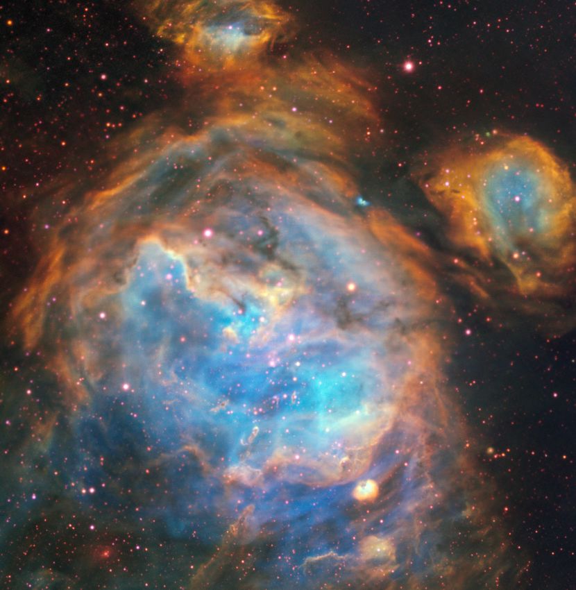
2                                                                     Jorge García-Rojas

nebulae was provided by Donald E. Osterbrock ([4]) who used a seminal paper by
Bowen ([5]) as the starting point for a review of nebular astrophysics.
   Photoionized nebulae are excited by the strong ultraviolet (UV) radiation of hot
stars (Te f f ≥ 25 − 30kK) which produce photons with energy that could be above
the ionization threshold of the gas particles and hence, ionize them releasing a
free electron. The probability of occurrence of this phenomenon depends on the
photoionization cross-section which, in turn, depends on the energy of the photon
and the target being considered. Once ionized, the gas particles tend to recombine
with the free electrons, and eventually an equilibrium stage is established in which
the rate of ionization equals the rate of recombination for each species (see [6]).
   The optical spectra of photoionized nebulae are dominated by emission lines,
which are formed when atoms or ions make a transition from one bound electronic
state to another bound state at a lower energy via spontaneous emission. These bound
electrons can be excited either by free electrons colliding with the atom/ion, or by
absorption of a photon. However, the background radiation field in the interstellar
medium in generally not strong enough for excitation by photon absorption to be
significant (see chapter 5 of [7]) and therefore, the only way of having a bound
electron in an excited state is by collisional excitation from a lower state, which
subsequent radiative decays to lower levels originating the collisionally excited lines
(hereinafter CELs), or owing to a recombination between a free electron and an ion,
which is the mechanism behind the emission of recombination lines (hereinafter
RLs). Given that the abundance of H and He ions are several orders of magnitude
higher than that of heavier elements, one can instinctively assume that the emission
spectra will be dominated by H and He lines, which is not the case. In photoionized
nebulae the peak of the energy distribution of free electrons is of the order of 1 eV.
Ions of heavy atoms like N, O, Ne, S, Cl, Ar, etc. have electronic structures with
low-lying electronic states in the range of fractions to few eV from the ground state
and can therefore be effectively excited by collisions. On the other hand, for H and
He ions, the gap between the ground state and the first excited state is very large
and cannot be excited by collisions, but by recombination. Fig. 1 shows a typical
optical spectrum of a photoionized nebulae (in this case the planetary nebula Hb 4);
remarkably bright H and He RLs and CELs of different ionic species of N, O, Ne,
S, Cl and Ar are labelled.
   Therefore, the spectrum of a photoionized nebula is dominated by the emission
of RLs of H and He (the most abundant elements) and CELs of heavier elements.
The combination of narrow-band images taken in the brightest emission lines allows
to construct the beautiful coloured images of photoionized nebulae (see Fig. 2) from
which we can have a first sketch of the ionization structure of the photoionized
region. In Fig. 2 we show a 3 narrow-band filter combined image of a star-forming
region in the Large Magellanic Cloud where is clear that the emission of [O iii] is
more internally located than the emission from [S ii].
   Although the emission line spectra from H ii regions and planetary nebulae
(hereinafter, PNe) are roughly similar, there are some remarkable differences between
them. H ii regions are large (tens of parsecs), massive (generally between 102 − 103
M ) regions of gas that are ionized by the ultraviolet (UV) radiation emitted by
Physical conditions and chemical abundances in photoionized nebulae                           3

Fig. 1 Section of the very deep spectrum of the PN Hb 4 analysed in [8, 9] showing bright RLs of
H i and He i and CELs of different ions of O, N, S and Ne.

recently formed OB-type massive stars with typical effective temperatures between
25-50 kK; in general, these stars are not hot enough to ionize nebular He ii, whose
ionization potential is hν = 54.4 eV. However, there are exceptions to this rule,
especially in the integrated spectra of blue compact dwarf galaxies (BCDs), Wolf-
Rayet (WR) galaxies and a couple of nebulae in the Local Group, associated to WR
stars. On the other hand, PNe are much smaller (10−1 pc) and less massive (∼10−1
M ) nebulae that are excited by central stars which are generally hotter (central
stars can reach temperatures as high as 250 kK); therefore, there will be ionizing
photons with enough energy to ionize high-excitation species and hence, producing
qualitatively different spectra than that of H ii regions, showing emission lines of
He ii, [Ne v], [Ar v], [Fe v], and even more excited species.

1.1 Why are abundances in photoionized nebulae important in
    astrophysics?

The analysis of emission line spectra of photoionized nebulae allows us to determine
the chemical composition of the interstellar medium (ISM) from the solar neigh-
bourhood to the high redshift star-forming galaxies. It stands as an essential tool for
our knowledge of stellar nucleosynthesis and the cosmic chemical evolution. Since
the early achievements in spectrophotometry of photoionized nebulae, the quality of
deep optical and near-infrared spectrophotometric data of PNe has increased signif-
icantly mainly thanks to both the development of more efficient instruments and to
the advent of large aperture (8m-10m-class) ground-based telescopes. In this sense,
4 Jorge García-Rojas
Fig. 2 “Bubbles of Brand New Stars” Composite image of a star-forming region in the Large
Magellanic Cloud (LMC) captured by the Multi Unit Spectroscopic Explorer (MUSE) instrument
on ESO’s Very Large Telescope (VLT). The following colour code was used: [O iii] λ5007 (blue).Hα
(yellow), [S ii] λ6731 (red). The field-of-view of the image is 7.82 × 8.00 arcminutes2 . North is
180.2deg left of vertical. Credit: ESO, A. McLeod et al.
the future installation of giant-class ones (diameters 30-50m) opens new horizons
in the field of nebular spectroscopy. The detection of very faint emission lines in
ionized nebulae as auroral CELs in faint, distant or high-metallicity objects; optical
recombination lines (hereinafter, ORLs) of heavy-element ions or CELs of trans-iron
neutron-capture elements are becoming a routine fact and provide new information
of paramount interest in many different areas of astrophysics.
H ii regions can be observed at considerable distances in the Universe and hence,
are crucial to determine the chemical composition of the interestellar medium (ISM)
in the extragalactic domain. Since H ii regions lie where star formation is occurring,
chemical abundances computed in H ii regions are probes to trace the present-Physical conditions and chemical abundances in photoionized nebulae 5 day chemical composition of the ISM. In particular, the study of radial variations of chemical abundances along galactic discs in spiral galaxies are essential obser- vational constraints for chemical evolution models, and precise determinations of chemical abundances in low-metallicity dwarf galaxies, can permit to determine the primordial abundance of helium owing to Big Bang nucleosynthesis (see [10] and references therein). The global picture of abundances in PNe is more complicated because for elements that are supposed to be not modified, such as O and α-elements, the computed abundances reflect the chemical conditions in the cloud where the pro- genitor star was formed, while the chemical abundances of N, C, or neutron-capture elements, that could be modified during the cycle of life of low-to-intermediate mass stars allow us to constrain the nucleosynthetic processes in these stars. 1.2 Recent reviews on chemical abundance determinations Recently, two tutorials focused on the determination of ionized gaseous nebulae abundances have been released ([10] and [11]) although with different points of view. In the former, [10] give a brief review on the physics basics of abundance determinations, like local ionization and local thermal equilibrium, emission line mechanisms and on the calculation of physical conditions and ionic and elemental abundance determinations from observations; these authors also review recent results in abundance determinations in both H ii regions and PNe. However the review is quite focused to the abundance discrepancy problem from the point of view of temperature fluctuations (see Section 4.5). In [11], the focus is on the determination of abundances in extragalactic H ii regions from the direct method (when electron temperature, Te , and electron density, ne , diagnostic lines are available) and in the use of some strong-line methods calibrated using the direct method (see Section 3.2). Further comprehensive tutorials on abundance determinations are those by [12] and [13] where the theoretical background of photoionized nebulae is treated in more detail, and particular emphasis is given to the description of line formation mechanisms, transfer of radiation, as well as to the use of empirical diagnostics based on emission lines and determination of chemical abundances using photoion- ization models. It is not the scope of this chapter to repeat the basic concepts of the physics of photoionized nebulae, which have been described in different detail in the aforementioned tutorials. Moreover, for a much more detailed description of such processes, we refer the reader to the canonical book of photoionized nebulae: “Astrophysics of gaseous nebulae and active Galactic nuclei” ([6]). In the following sections I will focus on recent advances in chemical abundances determinations in photoionized nebulae from the analysis of deep optical and near- infrared spectra, from an observational point of view. Due to space limitations, I refer the reader to [12, 13] for an overview on abundance determinations based on photoionization model fitting. Similarly, the strong line methods to determine abundances in the extragalactic domain (from giant H ii regions to high-redshift galaxies) will be only briefly discussed in Section 3.2.
6                                                                              Jorge García-Rojas

2 Observational spectroscopic data: the first step to obtain
  reliable abundances.

In the last years, the number of deep high-quality spectra of photoionized nebulae has
increased significantly, allowing the detection of very faint emission lines (see e. g.
[14, 15, 16, 17, 18, 19, 20, 8, 21, 22, 23]) and the computation of, in principle, very
reliable chemical abundances. The advantages of obtaining deep and high resolution
spectra of photoionized regions are clear because one can easily isolate faint lines that
in lower resolution spectra would be blended and go unnoticed. As an illustration, in
Fig. 3 we show an excerpt of the spectrum of the high-excitation PN H 1-50 analysed
in [24] with the same spectrum downgraded to a lower resolution overplotted in
red. Several permitted lines of O, N, and C would have remained hidden in the low-
resolution spectra and ad-hoc atomic physics would have been needed to estimate
their fluxes. In the last years, several groups have provided a large sample of deep,
high-resolution spectra of both Galactic and extragalactic H ii regions and PNe (see
e. g. [25, 26, 24] and the compilation made by [27]).

Fig. 3 Portion of a high-resolution (R∼15000) spectra of the high-excitation PN H 1-50 showing
the zone where the multiplet 1 O ii lines lie. Overplotted in red is the same spectra degraded to a
resolution of R∼3500. As it can be shown the high-resolution of the original spectra allows one
to deblend several very close permitted emission lines of C, O, and N that would have remained
hidden in the low-resolution spectra. Data originally published in [24].

   However, deep, high signal-to-noise, high-resolution spectra are not the panacea.
[28] has recently shown that the effects of observational uncertainties can be very
important even making use of high quality spectra, owing to the high number of
sources of uncertainty that are acting in the process, which include: assumptions in
the nebular structure, atomic data (see section 4.1), atmospheric differential refrac-
Physical conditions and chemical abundances in photoionized nebulae                    7

tion, telluric absorption and emission, flux calibration, extinction correction, blends
with unknown lines, etc. Therefore, a careful data reduction procedure should be
carried out to obtain reliable results. Additionally, an homogeneous analysis deter-
mining physical conditions and chemical abundances from the same set of spectra is
mandatory if one want to compute precise abundances. For instance, many studies
devoted to study the radial abundance gradients have made use of physical conditions
derived from radio recombination lines combined with and optical or infrared lines
to compute abundances; these approach has been used in several seminal papers on
the Galactic abundance gradient (see section 4.4; however, it can introduce system-
atic uncertainties owing to the different areas of the nebula covered in the different
wavelength ranges. Additionally, we should use a set of appropriate lines to com-
pute the abundances; as an example, computing O+ /H+ ratios from the trans-auroral
[O ii] λλ7320+30 lines could introduce undesired uncertainties because these lines
could be strongly affected by telluric emission, and are also very sensitive to electron
density and temperature. To illustrate these effects, in Fig. 4 we show an adaptation
of Fig. 5 of [29] where the radial oxygen abundance gradient making a consistent
analysis of several data sets is presented. Physical conditions have been derived from
both radio and optical diagnostics, and abundances have been derived using optical
CELs of oxygen (blue points) or far-IR fine-structure CELs of oxygen (red points).
As can be seen, both data sets show significant scatter in the oxygen abundance at
a given Galactocentric distance, which can be interpreted as an “intrinsic scatter”
owing to the gas not being well mixed ([30, 29, 31]). However, high-quality obser-
vations seem to rule out this interpretation. In Fig. 4 the abundances computed by
[32] from an homogeneous analysis of optical spectrophotometric data of 35 H ii
regions with direct determinations of the electron temperature have been overplotted
on the [29] sample. As it is clearly shown, the scatter in the oxygen abundance is
reduced significantly and is not substantially larger than the observational uncertain-
ties, indicating that oxygen seems to be well mixed in the ISM at a given distance
along the Galactic disc. Moreover, [33] showed from the analysis of high-quality
spectra with high signal-to-noise auroral [O iii] line detections in H ii regions in the
inner parts of M 33, a much lower scatter than that found by [31]; this author also
found no evidence for significant azimuthal variations in the H ii region metallicity
distributions, ruling out large anomalies in the mixing of the gas.
    Finally, one has to take into account some biases that the direct method can have.
[34] discussed about the limitations of the direct method to determine O abundances
in giant H ii regions at metallicities larger than solar. This author used ab-initio
photoionization models of giant H ii regions, and applied to the models the same
methods as used for real objects to test the direct method. The global result of this
study was that for log(O/H)+12 larger than 8.7 (i.e. larger than the solar value), the
computed O/H values were below the ones implied by the photoionization models
owing to strong temperature gradients present in giant H ii regions. Finally, [34]
propose that PNe, which are not affected by these biases, could be potential probes
of the metallicity of the interstellar medium in the internal parts of spiral galaxies as
well as in metal-rich elliptical galaxies. However, in Section 4.3 we will discuss that
this idea should be taken with some caution.
8 Jorge García-Rojas
Shaver et al. 1983 Afflerbach et al. 1997
10.5 Fich & Silkey 1991 Rudolph et al. 1997
Vilchez & Esteban 1996 Peeters et al. 2002
Caplan et al. 2000 Rudolph et al. 2006
10.0 Simpson et al. 1995 Esteban & Garcia-Rojas 2018
9.5
12+log(O/H)
9.0
8.5
8.0
7.5
7.0
0.0 2.5 5.0 7.5 10.0 12.5 15.0 17.5 20.0
RG (kpc)
Fig. 4 Radial oxygen abundance gradient in the MW using abundances derived from optical lines
(blue points) or from far-IR lines (red points) compiled by [29]. The data from [32] obtained through
deep spectra taken in 8m-10m class telescopes are overplotted (black squares). The fits for each
set of data are represented by lines with the same colour than the data points. References of the
original data compiled by [29] are shown in the legend.
3 Determination of physical conditions and ionic abundances
3.1 The direct method
The most popular way to compute the chemical abundances of the elements that are
present in a photoionized gas is the so-called direct method. This method makes use
of CELs intensities of different ionic species of elements like N, O, S, Ne, Cl, Ar, Ne,
Fe, etc., and involves the determination of the physical conditions (temperature and
electron density) in the emitting plasma. In the conditions prevailing in photoionized
nebulae like H ii regions and PNe, most of the observed emission lines are optically
thin1 with the exception of some resonance UV lines and some fine-structure IR
lines (see [12]) making their use for abundance determinations very robust.
1 An emission line is said to be optically thick if on average a photon emitted cannot pass through
the ISM without absorption. Conversely, an emission line is said to be optically thin if we can see
the radiation coming from behind the nebula (i. e. it is not absorbed).Physical conditions and chemical abundances in photoionized nebulae 9
In the analysis of photoionized nebulae it is usually assumed that the physical
conditions are homogeneous in the photoionized region. Under these assumptions
one can compute electron temperature and density by using sensitive line ratios.
Electron temperature (Te ) and density (ne ) in nebulae are represented by the kinetic
energy and density of the free electrons in the photoionized gas. Some CEL intensity
ratios of ions of common elements like O, N, S or Ar depend on the physical con-
ditions of the gas, and are useful to calculate Te and ne (see Section 3.5 of [10] for
more details). In particular, the intensity ratios of emission lines of a given ion that
originates in very different energy levels, are sensitive to Te and almost independent
on ne , since the populations of the different atomic levels are strongly dependent
on the kinetic energy of the colliding free electrons. Typical optical electron tem-
perature diagnostics are: [N ii] λ5754/λ6583, [O ii] λλ7320+30/λλ3726+29, [O iii]
λ4363/λ5007, [Ar iii] λ5191/λ7531 or [S iii] λ6312/λ9531. Therefore, determina-
tion of chemical abundances making use of the direct method in optical spectra
requires the detection of faint auroral lines, which correspond to transitions from the
state 1 S to 1 D and are very Te -sensitive. The detection of such lines is a relatively easy
task in Galactic H ii regions and PNe. However, their emissivity decreases rapidly
with metallicity and with decreasing surface brightness of the objects so, detecting
them is a challenging task in the extragalactic domain, especially in objects beyond
the Local Group. However, the combination of high-sensitivity spectrographs with
large aperture (10m type) telescopes have allowed the detection of the auroral [O iii]
λ4363 Å line in at least 18 star-forming galaxies at z > 1 (see [35] and references
therein).
On the other hand, line ratios sensitive to ne come from levels with very similar
energy, so that the ratio of their populations does not depend on Te . These levels
show different transition probabilities or different collisionally de-excitation rates,
such that the ratio between the emission lines generated is strongly dependent on the
electron density of the photoionized gas. Typical optical density diagnostics are: [O ii]
λ3726/λ3729, [S ii] λ6716/λ6731, [Cl iii] λ5517/λ5537 and [Ar iv λ4711/λ4741.
A precise determination of the physical conditions is crucial to derive reliable
abundances from CELs. As the abundances are computed relative to H by using
the relative intensities of CELs or ORLs relative to a H i ORL (usually Hβ), and
given the very different dependence of the emissivity of CELs and ORLs (see [10])
the abundances from CELs show a strong (exponential) dependence on Te , while
abundances computed from faint metallic ORLs are almost Te dependent. This
has important implications for the so-called abundance discrepancy problem (see
Section 4.5).
Once physical conditions are computed one has to decide the temperature and
density structure that is going to be assumed in the nebula. The most common
approach, is to assume a two-zone scheme, where the high ionization zone is char-
acterized by Te (high) (usually Te ([O iii]), the low-ionization zone is characterized
by Te (low) (usually Te ([N ii]) and the density is considered homogeneous in the
whole nebula and is characterized by ne ([S ii]). Then, each temperature is applied
to compute ionic abundances of species with similar ionization potentials than the
ion used in the Te diagnostic. In a typical spectra, Te (low) is applied to compute10 Jorge García-Rojas
abundances of N+ , O+ , S+ , Cl+ and Fe+ , while Te (high) is used for the remaining
ionic species observed in the optical spectra.
However, recent results from [36] have shown that this scheme can be erroneous.
These authors, from deep, high-resolution spectra of H ii regions in the Magellanic
Clouds, have proposed that for some ions, it is better to adopt other scheme in order to
avoid trends with metallicity. In particular, they propose to use Te ([N ii]) to calculate
Cl2+ and the mean of Te ([N ii]) and Te ([O iii]) for S2+ and Ar2+ , finding that, in such
cases, Cl/O, S/O and Ar/O are approximately constant with metallicity (see their
Fig. 3) as expected for α-elements.
In deep spectra, covering the whole optical (or even up to 1µm) wavelength range
more electron temperature and density diagnostics will be available. In such cases,
Te (low) and Te (high) can be computed as the average of the values obtained from
different diagnostics, which are generally in reasonable good agreement within the
uncertainties (see e. g. [15, 37, 19]). In some cases, particularly in relatively high-
density PNe (ne > 104 cm−3 ), density stratification can be observed, with the [Ar iv]
densities being larger than those computed with the other three diagnostics (see [38]).
In such cases it is better to consider also a two-zone density model (see [9]). In some
extreme cases of extremely young and dense PNe, with densities higher than the
critical densities of the upper levels of the transitions producing the [Ar iv] lines, all
the classical electron density diagnostics will be saturated and can provide inaccurate
densities. An alternative density indicator is based on the analysis of [Fe iii] emission
lines, which are robust density diagnostics when collisional de-excitation dominates
over collisional excitation. Indeed, if inappropriate density diagnostics are used, then
physical conditions deduced from commonly used line ratios will be in error, leading
to unreliable chemical abundances for these objects. (see [39]).
3.1.1 Analysis tools
The first public code for the computation of physical conditions and ionic abundances
was fivel [40], an interactive FORTRAN program which used a basic five-level atom
approximation, which considers that only the five low-lying levels (i. e. at energies
≤5 eV above the ground state are physically relevant for computing the observed
emission line spectrum. Later, [41] developed nebular, a set of software tools
(based in the fivel program, but extending it to an N-level atom) in the iraf/stsdas2
environment that allow the user to compute diagnostic for a variety of ground-state
electron configurations, and compute ionic abundances separately for up to 3 zones
of ionization. The main advantage of nebular is that it can be scripted. However,
changes of atomic data sets is not trivial and computations of elemental abundances
are not included.
2 iraf is distributed by National Optical Astronomy Observatories, which is operated by AURA
(Association of Universities for Research in Astronomy), under cooperative agreement with NSF
(National Science Foundation).Physical conditions and chemical abundances in photoionized nebulae 11
([42]) developed the Nebular Empirical Analysis Tool (neat3), a very simple to
use code written in FORTRAN90 which requires little or no user input to return
robust results, trying to provide abundance determinations as objective as possible.
One of the main advantages of this code is that it can evaluate uncertainties of the
computed physical conditions and abundances by using a Monte Carlo approach.
Another advantage of this code is that it also accounts for the effect of upward
biasing on measurements of lines with low signal-to-noise ratios, allowing to reduce
uncertainties of abundance determinations based on these lines. Finally, as atomic
data for heavier elements than helium are stored externally in plain text files, the user
can easily change the atomic data.
The last package to be offered in the field has been PyNeb4 ([43]) which is
completely written in python and is designed to be easily scripted, and is more
flexible and therefore, powerful than its predecessors. This package allow the user to
easily change and update atomic data as well as providing tools to plot and compare
atomic data from different publications.
3.2 Abundances in distant photoionized nebulae: the strong line
methods
In the absence of reliable plasma diagnostics (a common fact in extragalactic objects)
in giant H ii regions or integrated spectra of galaxies, one needs to use alternative
methods to derive accurate chemical abundances. This is especially important to
estimate the metallicities of giant extragalactic H ii regions as well as of local and
high-redshift emission-line galaxies and hence, it has a relevant influence on the
study of the chemical evolution of the Universe.
The first mention of the strong-line methods was 40 years ago, when [44] and
[45] proposed a method to compute the oxygen abundance using strong lines only:
the R23 method, in which oxygen abundance is a one dimensional function of the
R23 parameter, defined as:
[OII]λ3727 + [OIII]λ4959 + 5007
R23 = (1)
Hβ
This method was calibrated using the few relevant photoionization models avail-
able at that time. The problem with dealing with R23 is that it is double valued with
respect to metallicity. In fact, at low oxygen abundances –12+log(O/H) . 8.0– the
R23 index increases with the abundance, while for high oxygen abundances –12 +
log(O/H) ≥ 8.25– the efficiency of the cooling caused by metals make R23 to drop
with rising abundance. There is also a transition zone between 8.0 and 8.25 (see e. g.
[46] for a detailed description of the high and low metallicity branches). This method
has been refined multiple times since then and several calibrations, using data sets
3 https://www.nebulousresearch.org/codes/neat/
4 https://github.com/Morisset/PyNeb_devel12 Jorge García-Rojas with abundances from the direct method (e. g. [46, 47]), using photoionization model grids (e. g. [48, 49]), or a combination of both, are now available in the literature. An overview of the most popular calibrations of strong-line methods can be found in [50]. A comprehensive critical evaluation of the different semi-empirical strong-line methods has been done by [51] who also develop a method for reducing systematics in the techniques to compute chemical abundances by using electron temperatures and ionization correction factors. In the last years, mainly thanks to the increasingly easy access to super-computing resources, new approaches have been proposed. Bayesian methods have been used by several authors to determine chemical abundances in extragalactic targets (e. g. [52]) although the priors should be selected cautiously to avoid unreliable results. On the other hand, as in most of astronomy fields, machine learning techniques are also being used to infer chemical abundances (see e. g. [53]). However, as has been pointed out by [54], making use of an illustrative example, the use of these techniques ignoring the underlying physics can lead to unphysical inferences. [54] have argued in a comprehensive review that although strong-line methods are routinely used to estimate metallicities owing to their apparent simplicity, the users need to have a solid background on the physics of H ii regions to understand the approximations made on the different approaches, and the limitations each calibration has, to avoid biases, misinterpretations and mistakes. Even taking into account the drawbacks mentioned above, strong-line methods have been widely used for studying giant H ii regions and emission line galaxies in large long-slit spectroscopic surveys as the Sloan Digital Sky Survey (SDSS) [55], or 2D spectroscopic surveys as MANGA (e. g. [56, 57]), CALIFA (e. g. [58]), and AMUSING (e. g. [59]). 4 Advances in abundances determinations in photoionized nebulae In this section I will focus on the latest advances that have been reached in the field of photoionized nebulae. I will pay special attention to atomic data, ionization cor- rection factors and the abundance discrepancy problem, that have been traditionally claimed as potential sources of uncertainty in chemical abundance determinations. 4.1 Atomic data The atomic data used for computing abundances in photoionized nebulae are ususally considered as a black box by the users. Most users consider the default atomic data sets used by their favourite analysis tools or directly use the last available atomic data in the literature for each ion. In the last years large compilations of atomic data
Physical conditions and chemical abundances in photoionized nebulae                  13

have been done in the chianti5 and nist6 databases, although the available atomic
data in each database do not always match for a given ion. [60, 61] discussed how to
ensure that atomic data are correctly understood and used, as well as on the typical
uncertainties in atomic data.
    High-quality observations of photoionized nebulae are a powerful tool to check
the reliability of atomic data. [62] and [38] found, using a large data set of PNe
spectra and comparing electron density estimates for PNe based on different density
diagnostics, that the [O ii] transition probabilities calculated by [63] yielded system-
atically lower electron densities than those computed using the [S ii] diagnostic, and
that such discrepancies were caused by errors in the computed transition probabili-
ties. Moreover, [38] found that the transition probabilities of [64] and the collision
strengths of [65] were completely inconsistent with observations at the high and low
density limits, respectively, and should be ruled out.
    [66] determined chemical abundances of O, N, S, Ne, Cl and Ar for a sample of
PNe and H ii regions and evaluated the impact of using different sets of atomic data
on the computed physical conditions and abundances. These authors used all the
possible combinations of 52 different sets of transition probabilities and collision
strengths to calculate physical conditions and chemical abundances, finding that
different combinations of atomic data introduce differences in the derived abundances
that can reach or surpass 0.6-0.8 dex at higher densities (ne > 10−4 cm−3 in several
abundance ratios like O/H and N/O. Removing the data sets that introduce the largest
differences can reduce the total uncertainties, although they can still remain in high-
density objects. Additionally, they have pointed out that special attention should be
paid to the transition probabilities of the S+ , O+ , Cl++ and Ar3+ density diagnostic
lines, and to the collision strengths of Ar3+ which, if incorrectly selected, can lead
to unreliable chemical abundances in high-density nebulae.
    Finally, [54] has pointed out that the role of atomic data in strong-line method
calibrations cannot be ignored. Recent changes in routinely used atomic data have
revealed that they play a crucial role in direct abundance determinations and in
photoionization models.

4.2 Ionization correction factors

The elemental abundance of a particular element is computed by adding up the ionic
abundances of all the ions present in a nebula. However, it is usually found that
not all the ions of a given element are observed, whether because they are emitted
in a different spectral range than that observed or because the spectra is not deep
enough to detect them. Therefore, the contribution of these unobserved ions should
be estimated in someway. With this aim, the use of Ionization Correction Factors
(ICFs) was proposed by [67]. These authors proposed to use similarities between

5 http://www.chiantidatabase.org
6 http://physics.nist.gov
14 Jorge García-Rojas ionization potentials of different ions to construct ICFs. This approach has been used by several authors since then (see e. g. [68]). However, [12] argued that these ICFs should be treated with caution because the ionization structure in a photoionized nebula does not depend only on the ionization potential. Moreover, it has been shown that using recent photoionization models, these simple expressions are not always valid and new ICFs are needed to obtain more reliable abundances (see e. g. [69]) The alternative is to compute ICFs using photoionization models, where the physics involved in ionized nebulae is treated with much more detail. Photoioniza- tion models allow to compute the detailed ionization structure of the various elements present in a nebula, by taking into account all the processes that govern ionization and recombination (i.e. mostly photoionization, radiative and di-electronic recom- bination, and charge exchange), as well as all the heating and cooling processes that determine the electron temperature ([70]). Traditionally, different ICFs have been computed for H ii regions and PNe, given the differences in the hardness of the radiation field and the different ionic species detected in each type of object (see Section 1). Several authors have derived ICFs from photoionization models for H ii regions ([71, 72, 73, 74, 75, 76, 77]) and for PNe ([78, 79, 70]). It is not the scope of this text to show the details of the different approaches used to compute ICFs from photoionization models, but I think it is worth mentioning some of the most widely used ICF schemes. [75] re-evaluated empirical expressions for the abundance determination of N, O, Ne, S, Cl, Ar and Fe to compute abundances of emission-line galaxies from the Data Release 3 of the Sloan Digital Sky Survey (SDSS). They took special care in the selection of atomic data and constructed an appropriate grid of photoionization models with state-of- the art model atmospheres. In particular, these authors take care of a problem that should not be ignored in the computation of photoionization models, which is the uncertain rate of the dielectronic recombination for sulfur, chlorine and argon ions. They compared the abundances of these elements calculated with different assumed dielectronic recombination rates and could put some constraints on these rates. Additionally, following an approach that was defined by [80] these authors proposed different ICFs depending on the metallicity range of the nebulae. Regarding PNe, [70] constructed ICFs for He, N, O, C, Ne, S, Cl, and Ar using a large grid of photoionization models that are representative of most of the observed PNe. Besides the obvious advantage of covering a wide range of physical parameters with a large photoionization model grid, the main advantage of this work is the provision of analytical expressions to estimate the uncertainties arising from their computed ICFs. Finally, a third scheme to compute ICFs is to derive analytical expressions ob- tained from observational fittings to large sets of high-quality data (see e. g. [81] for Cl, and [82] for C). In section 4.7.2 I will come back to the ICFs mentioning some works devoted to the computation of ICFs for neutron-capture elements in PNe.
Physical conditions and chemical abundances in photoionized nebulae                               15

4.3 Oxygen enrichment in PNe

Oxygen is the element for which more reliable abundances can be obtained and,
therefore, it has been traditionally used as a proxy for metallicity. In H ii regions,
oxygen reflects the current abundance in the ISM, while in PNe, it is supposed to
reflect the chemical composition of the environment where the star was born because
its abundance remain unchanged during the life of the star ([83]). However, AGB
stars can modify the oxygen abundance by two mechanisms: the third dredge-up
(TDU) and the hot bottom burning (HBB), although only nucleosynthesis models
which include extra-mixing processes like diffusive convective overshooting (e. g.
[84, 85, 86]) predict a significant production of oxygen.

            4.0
                         CRD
            3.8
                         ORD
                         H II regions
            3.6
    log(O/Cl)

            3.4

            3.2

            3.0

            2.8
               7.8        8.0          8.2          8.4          8.6          8.8          9.0
                                             12+log(O/H)
Fig. 5 Values of O/Cl as a function of O/H for a sample of Galactic PNe and H ii regions (see [83]).
The red circles represent PNe with oxygen-rich dust, the green diamonds PNe with carbon-rich
dust, and the blue stars the H ii regions. The protosolar abundances of [87] are overplotted with the
solar symbol. Plot made with data gently provided by Gloria Delgado-Inglada.

   Until recently, the only observational probes of oxygen production in AGB stars
have been restricted to low-metallicity PNe (see e. g. [88]). However, using deep,
high-quality optical spectra (with spectral resolution better than 1 Å) [83] recomputed
accurate abundances of He, O, N, Ne, C, Ar, and Cl in 20 PNe and 7 H ii regions
in our Galaxy at near-solar metallicities. These authors found that all but one of the
Galactic PNe with C-rich dust (the one with the highest metallicity according to
16 Jorge García-Rojas
Cl/H) show higher O/Cl values than the PNe with O-rich dust and the H ii regions
(see Fig. 5), and interpret that result as O is enriched in C-rich PNe due to an efficient
third dredge-up in their progenitor stars. These results have been confirmed later by
nucleosynthesis models including convective overshooting by [85, 89].
These findings confirm that oxygen is not always a good proxy of the original ISM
metallicity and other chemical elements such as chlorine or argon, the abundance of
which is unaltered in the evolution of low- and intermediate-mass stars, should be
used instead. Additionally, as has been pointed out by [89], the production of oxygen
by low-mass stars should be thus considered in galactic-evolution models.
4.4 Abundance gradients in the Milky Way and in nearby spiral
galaxies from direct abundance determinations
The study of the radial distribution of the gas phase metallicity in a Galaxy (usually
using oxygen as a proxy for the metallicity) is fundamental for our understanding
of the evolution of Galaxies. The pioneering studies on the gradient of abundances
in spiral galaxies were those of [90] and [91], which were based on the spectral
differences found by [92] between the H ii regions in the spiral galaxy M33. [93]
were the first in carrying out an homogeneous study of abundance gradients in the
Milky Way (hereinafter, MW) with a relatively large sample of H ii regions. How-
ever, these authors rely on electron temperatures determined from radio RLs and
abundances from optical lines, obtaining a relatively large scatter at a given Galacto-
centric distance. Since these pioneering works, several authors have computed radial
abundance gradients using the direct method in our Galaxy (e. g. [94, 95, 29, 96, 97])
and in external galaxies (see e. g. [98, 99, 100, 101, 25] and references therein).
Regarding the MW, the relatively large scatter at a given Galactocentric distance
found in several works has been claimed as a possible indication that the gas is
not as well mixed as commonly thought (see e. g. [29]). Moreover, [102] found
significant differences in the radial gradient of O in the MW depending on the
Galactic azimuth region considered, strengthening the idea that metals are not well
mixed at a given radius. However, [32] made an homogeneous analysis using a set of
deep optical spectra of 35 H ii regions, from which they computed accurate physical
conditions and ionic and elemental abundances, finding that the scatter of the N
and O abundances of H ii regions is of the order of the observational uncertainties,
indicating that both chemical elements seem to be well mixed in the ISM at a given
Galactocentric distance (see the comparison between radial O abundance from this
work and that of [29] in Fig. 5).
In the extragalactic domain, it is worth mentioning the existence of the CHemical
Abundances of Spirals (CHAOS) project, which is devoted to surveying several
spiral galaxies to determine precise “direct” abundances in large samples of H ii
regions in spiral galaxies (see [101, 100, 103]). This project has increased by more
than an order of magnitude the number of H ii regions with direct measurements of
the chemical abundances in nearby disk galaxies (see [101]).Physical conditions and chemical abundances in photoionized nebulae 17
There are many open problems with the abundance gradients of the MW and
nearby spiral Galaxies such as a possible temporal evolution ([104, 105]) based on
the differences found in the gradients using different populations of PNe and H ii
regions; the existence or not of a flattening of the gradient in the outer disc of spiral
galaxies, including the MW ([106, 96, 59]) or in the inner disc ([96, 59]); distance
determinations uncertainties, particularly for PNe (see [105]) or, as mentioned in
section 4.3, the applicability of oxygen as a reliable element to trace the metallicity
in PNe ([83]). Some of the limitations that, in my opinion should be taken into
account have been summarized in [107].
The determination of precise radial metallicity gradients are precious constraints
for chemical evolution models of the MW in particular and of spiral galaxies in
general. The presence of a negative gradient agrees with the the stellar mass growth
of galaxies being inside-out (see e. g. [108]). However, additional information, such
as the possible temporal evolution of the gradients (see e. g. [104, 105]) can give
information about physical processes that can modify gradients, and that should be
considered by chemical evolution models (see discussion by [105] and references
therein). As H ii regions reflect the young stellar populations and, on the other
hand PNe, reflect older stellar populations (with a relatively large spread in ages) a
careful comparison between gradients obtained from different objects is very useful
to constrain the temporal evolution of the gradient predicted by chemical evolution
models ([109]).
4.5 The abundance discrepancy problem
The abundance discrepancy problem is one of the major unresolved problems in
nebular astrophysics and it has been around for more than seventy years ([110]). It
consists in the fact that in photoionized nebulae −both H ii regions and PNe− ORLs
provide abundance values that are systematically larger than those obtained using
CELs. Solving this problem has obvious implications for the measurement of the
chemical content of nearby and distant galaxies, because this task is most often done
using CELs from their ionized ISM.
For a given ion, the abundance discrepancy factor (ADF) is defined as the ratio
between the abundances obtained from ORLs and CELs, i. e.,
ADF(X i+ ) = (X i+ /H + )ORLs /(X i+ /H + )CE Ls, (2)
and is usually between 1.5 and 3, with a mean value of about 2.0 in H ii regions
and the bulk of PNe (see e.g. [111, 27], but in PNe it has a significant tail extending
to much larger values, up to 2–3 orders of magnitude7. It is important to remark
that the ADF is most easily determined for O2+ owing to both CELs and RLs are
straightforward to detect in the optical. ADFs can be also determined for other ions,
7 An updated record of the distribution of values of the ADF in both H ii regions and PNe can be
found in Roger Wesson’s webpage: http://nebulousresearch.org/adfs18 Jorge García-Rojas such as C2+ , N2+ , and Ne2+ , although the obtained values are more uncertain because CELs and RLs are detected in different wavelength ranges (in the case of C2+ and N2+ ) or because RLs are intrinsically very faint (in the case of Ne2+ ). The possible origin of this discrepancy has been discussed for many years and three main scenarios have been proposed: • [112] was the first proposing the presence of temperature fluctuations in the gas to explain the discrepancy between Te ([O iii]) and Te (H I) derived from the Balmer jump. After that seminal work, [67] developed a scheme to correct the abundances computed from CELs for the presence of temperature inhomogeneities. Later, [113] suggested that the discrepancy between ORLs and CELs abundances could be explained if spatial temperature variations over the observed volume were considered. [10] have recently summarized the mechanisms proposed to explain and maintain the presence of temperature fluctuations in photoionized nebulae. • [114] were the first in proposing the existence of chemical inhomogeneities in the gas as a plausible mechanism to explain the abundance discrepancy. This scenario was later expanded by [14], who claimed that metal-rich (i. e. H-poor) inclusions could be the clue to resolve the abundance discrepancy problem; in this scenario, metal ORLs would be emitted in the metal-rich inclusions, where cool- ing has been enhanced, while CELs would be emitted in the “normal” metallicity (H-rich) zones. This model was tested by several authors by constructing two- phase photoionization models that, in several cases, successfully simultaneously reproduced the ORLs and CELs emissions in H ii regions [115] and PNe [116]. However, at the present time, the origin of such metal-rich inclusions remains elusive, although some scenarios have been proposed for PNe ([117]) and H ii regions ([118]). In the last years, increasing evidence has been found of a link between the presence of a close central binary star at the heart of PNe and very high (>10) ADFs (see Section 4.5.1). • A third scenario was brought into play by [119], who proposed that the departure of the free electron energy distribution from the Maxwellian distribution (κ- distribution) could explain the abundance discrepancies owing to the presence of a long tail of supra-thermal electrons that contribute to an increase in the intensity of the CELs at a given value of the kinetic temperature. However, in the last years little theoretical ([120, 121, 122]) or observational ([123]) support has been presented for this scenario in photoionized nebulae. [121] have shown that the heating or cooling timescales are much longer than the timescale needed to thermalize supra-thermal electrons because they can only travel over distances that are much shorter than the distances over which heating rates change, implying that the electron velocity distribution will be close to a Maxwellian one long before the supra-thermal electrons can affect the emission of CELs and RLs. Moreover, [122] demonstrated analytically that the electron energy distribution relaxes rapidly to a steady-state distribution that is very close to a Maxwellian, having negligible effects on line ratios. One of the most active groups in the study of the abundance discrepancy in PNe in the last two decades has been the University College London/U. Beijing group,
Physical conditions and chemical abundances in photoionized nebulae                 19

who have developed deep medium-resolution spectrophotometry of dozens of PNe
to compute the physical and chemical properties of these objects from ORLs. In
one of the most detailed and comprehensive studies of this group, [124] showed
that the values of the ADF deduced for the four most abundant second-row heavy
elements (C, N, O and Ne) are comparable (see their Fig. 18). However, they also
computed abundances from ORLs from a third-row element (Mg) and they found
that no enhancement of ORL abundances relative to CEL ones is obvious for Mg: the
average Mg abundances from ORLs for disk PNe remained in a range compatible to
the solar photospheric value, even taking into account the small depletion expected
for this element onto dust grains (less than 30%). Finally, these authors also showed
that, regardless of the value of the ADF, both CEL and ORL abundances yield similar
relative abundance ratios of heavy elements such as C/O, N/O and Ne/O . This has
important implications, especially in the case of the C/O ratio, given the difficulties
of obtaining this ratio from UV CELs (see Sect. 4.6).
    Several authors have strongly argued in favour of the inhomogeneous composition
of PNe and against pure temperature fluctuations (see e. g. [125] and references
therein); some of the reasoning that has been presented supporting this model are: i)
far-IR [O iii] CELs, which in principle, have a much lower dependence on electron
temperature than optical CELs, provide abundances that are consistent with those
derived from optical CELs (see e. g. [14]); ii) the analysis of the physical conditions
using H, He, O and N ORLs yields electron temperatures that are much lower than
those computed from classical CEL diagnostic ratios (see [126, 127, 128, 20]);
additionally, ORL density diagnostics provide densities that are higher than those
derived from CEL diagnostics; iii) chemically homogeneous photoionization models
do not reproduce the required temperature fluctuations to match CEL and ORL
abundances, while bi-abundance photoionization models including an H-poor (i. e.
metal-rich) component of the gas successfully reproduce the observed intensities of
both CELs and ORLs (e. g. [116]). All these arguments strongly favour the presence
of a low-mass component of the gas that is much colder and denser than the “normal”
gas, and that is responsible for the bulk of the ORL emission. However, we cannot rule
out the possibility that different physical phenomena can contribute simultaneously
to the abundance discrepancy in PNe.
    Some physical phenomena have been proposed to explain the abundance dis-
crepancy in the framework of temperature fluctuations or chemical inhomogeneities
scenarios ([117, 10]). However, until very recently, there was no observational proof
that demonstrated a single physical process to be responsible for the abundance dis-
crepancy. Some recent works on the Orion nebula have observationally linked the
abundance discrepancy to the presence of high velocity flows ([129]) or to the pres-
ence of high density clumps, such as proto-planetary disks ([130, 39]. On the other
hand, [125] found a very extreme value of the ADF for the PN Hf 2–2 (ADF∼70)
and, for the first time, suggested the possibility that this large ADF could be related
to the fact that the central star of the PN, which is a close-binary star, has gone
through a common-envelope phase.
20 Jorge García-Rojas
4.5.1 The link between close binary central stars and large abundance
discrepancy factors
Several papers in recent years have confirmed the hypothesis proposed by [125] that
the largest abundance discrepancies are reached in PNe with close-binary central
stars. [131] found that three PNe with known close-binary central stars showed high
ADFs, with the PN Abell 46, with an ADF(O2+ )∼120, and as high as 300 in its inner
regions, being the most extreme object. Their spectroscopic analysis supports the
previous interpretation that, in addition to “standard” hot (Te ∼104 K) gas, a colder
(Te ∼103 K), metal-rich, ionized component also exists in these nebulae. Both the
origin of the metal-rich component and how the two gas phases are mixed in the
nebulae are basically unknown. Moreover, this dual nature is not predicted by mass-
loss theories. However, it seems clear that the large-ADF phenomena in PNe is linked
to the presence of a close-binary central star. In fact, [23] have recently completed
a survey of the ADFs in seven PNe with known close-binary central stars and they
found ADFs larger than 10 for all of them, confirming the strong link between large
ADFs and close-binary central stars. On the other hand, several spectroscopic studies
have shown that the ORL emitting plasma is generally concentrated in the central
parts of the PNe. This occurs in PNe with known close-binary central stars and
large ADFs (e. g. [131, 132]), in PNe with low-to-moderate ADFs and no indication
of binarity (e. g. [133, 134]) and in PNe with relatively large ADFs but no known
close-binary central star (e. g. M 1–42, see [135]).
[136] recently obtained the first direct image of the PN NGC 6778 (a PN with
ADF∼20) in O ii recombination lines, taking advantage of the tunable filters available
at the OSIRIS instrument in the 10.4m Gran Telescopio Canarias (GTC). They found
that in NGC 6778, the spatial distribution of the O ii λλ4649+50 ORL emission does
not match that of the [O iii] λ5007 CEL. [135] found the same behaviour in Abell 46
using direct tunable filter images centred at λλ4649+51 Å.
Moreover, [135] presented preliminary results obtained from deep 2D spectro-
scopic observations with MUSE at the 8.2m Very Large Telescope (VLT) of five
southern large-ADF PNe, and they confirmed this behaviour in at least the PNe
Hf 2-2 (ADF∼84), M 1-42 and NGC 6778 (both with ADF∼20). In Fig 6 we show
the MUSE emission line maps of several emission lines in the PN NGC 6778. The
emission maps are ordered by increasing ionization potential of the parent ion from
left to right and from top to bottom. It is clear that O ii λ4649+50 ORLs emission
is more centrally concentrated that [O iii] λ4959 CEL emission, and seems to be
emitted in a zone that correspond to a higher ionization specie. A similar result has
been found by [137] from a kinematical analysis of several heavy metal ORLs and
CELs in NGC 7009. These authors found that the kinematics of ORLs and CELs
were discrepant and incompatible with the ionization structure of the nebula, unless
there is an additional plasma component to the CEL emission that arises from a dif-
ferent volume from that giving rise to the RL emission from the parent ions within
NGC 7009. Similarly, [138] found that the kinematics of the C ii λ6578 line is not
what expected if this line arises from the recombination of C2+ ions or the fluores-
cence of C+ ions in ionization equilibrium in a chemically homogeneous nebularPhysical conditions and chemical abundances in photoionized nebulae 21 Fig. 6 MUSE Emission line maps of several lines in the PN NGC 6778, ordered by ionization potential of the parent ion: from left to right and from top to bottm: [O i] λ6300 Å, [S ii] λ6731 Å, Hβ λ4861 Å, [N ii] λ6548 Å, He i λ5876 Å, O ii λλ4649+50 ÅORLs, [O iii] λ4959 ÅCEL, [Ar iv] λ4740 Åand He ii λ4686 Å. It is worth re-emphasising that the O ii and the [O iii] emission comes from the same ion: O2+ . The “x” marks a reference spaxel plasma, but instead its kinematics are those appropriate for a volume more internal than expected. These results clearly support the hypothesis of the existence of two separate plasmas, at least in these large-ADF PNe, with the additional indication that they are not well mixed, perhaps because they were produced in distinct ejection events related to the binary nature of the PN central star. [23] propose that a nova-like outburst from the close-binary central star could be responsible for ejecting H- deficient material into the nebulae soon after the formation of the main nebula. This material would be depleted in H, and enhanced in C,N, O, and Ne, but not in third row elements. It is worth mentioning the similarity of these plasma component with some well-known old nova shells as CP Pup and DQ Her that show low Te and strong ORLs ([139, 140]).
You can also read