Plugged-in Electric Vehicle-Assisted Demand Response Strategy for Residential Energy Management

Plugged-in Electric Vehicle-Assisted Demand
Response Strategy for Residential Energy
Management
Khaldoon Alfaverh (  khaldoonalfaverh@edu.bme.hu )
 Budapest University of Technology and Economics
Fayiz Alfaverh
 University of Hertfordshire
Laszlo Szamel
 Budapest University of Technology and Economics

Research Article

Keywords: Fuzzy Logic Controller, Home Energy Management System, Energy Storage Systems, Vehicle-
to-Home, Smart Home, Smart Grid

Posted Date: January 4th, 2023

DOI: https://doi.org/10.21203/rs.3.rs-2424104/v1

License:   This work is licensed under a Creative Commons Attribution 4.0 International License.
Read Full License

Additional Declarations: No competing interests reported.

Plugged-in Electric Vehicle-Assisted Demand Response Strategy for
Residential Energy Management
Khaldoon Alfaverh1*, Fayiz Alfaverh2 , Laszlo Szamel1

 1 Department of Electric Power Engineering, Faculty of Electrical Engineering and Informatics, Budapest University of Technology and
 Economics, H-1521 Budapest, P.O.B. 91, Hungary
 2 School of engineering and computer science, University of Hertfordshire, AL10 9AB, Hatfield, United Kingdom
*
 Corresponding author, e-mail: khaldoonalfaverh@edu.bme.hu

Abstract

Demand response (DR) management systems are a potentially growing market due to their ability to maximize energy
savings by allowing customers to manage their energy consumption at times of peak demand in response to financial
incentives from the electricity supplier. Successful execution of a demand response program requires an effective
management system where the home energy management system (HEMS) is a promising solution nowadays. HEMS
is developed to manage energy use in households and to conduct the management of energy supply, either from the
grid or the alternative energy sources like solar or wind power plants. With the increase of vehicle electrification, in
order to achieve a more reliable and efficient smart grid (SG), cooperation between electric vehicles (EVs) and
residential systems is required. This cooperation could involve not only vehicle to grid (V2G) operation but a vehicle
to home (V2H) too. V2H operation is used to transfer the power and relevant data between EVs and residential
systems. This paper provides an efficient HEMS enhanced by smart scheduling and an optimally designed charging
and discharging strategy for plugged-in electric vehicles (PEVs). The proposed design uses a fuzzy logic controller
(FLC) for smart scheduling and to take the charging (from the grid)/discharging (supply the household appliances)
decision without compromising the driving needs. Simulations are presented to demonstrate how the proposed
strategies can help to reduce electricity costs by 19.28% and 14.27% with 30% and 80% state of charge (SOC) of the
PEV respectively compared to the case where G2V operation only used along with the photovoltaic (PV) production,
improve energy utilization by smoothing the energy consumption profile and satisfy the user’s needs by ensuring
enough EV battery SOC for each planned trip.

Keywords

Fuzzy Logic Controller, Home Energy Management System, Energy Storage Systems, Vehicle-to-Home, Smart
Home, Smart Grid.

Nomenclature
 
 V2H Vehicle to home Rated capacity of PEV battery
 ℎ 
 G2V Grid to vehicle Maximum PEV charging power
 − ℎ Rated power of non-shiftable appliances 
 Maximum PEV discharging power
 ℎ Rated power of shiftable appliances ℎ
 PEV charging power

 ( ) Status of non-shiftable appliances 
 PEV discharging power
 ( ) Status of shiftable appliances ( ) Real time electricity price
 ( ) Total power usage of household appliances ( ) Energy of PEV battery
 
 Lower limit of average total power demand Status of PEV
 
 Upper limit of average total power demand ( ) State of charge of PEV battery
 ℎ _ ( ) Required shifting power Arrival time of PEV
 _ _ ( ) Required valley filling power Departure time of PEV
 ℎ 
 Shifting probability of shiftable appliances ( ) Consumed power from grid
 _ 
 Valley filling probability

1. Introduction
The demand for electricity due to industrialization and the shift from conventional grids to smart ones is exponentially
growing nowadays. Meanwhile, the use of renewable energy sources (RESs), EVs, and energy storage systems (ESSs)
is also increasing. To influence customer use of electricity in ways that will produce desired changes in the utility's
load profile, demand side management (DSM) is used for those utility designed activities. Moreover, time-of-use
pricing (TOU) encourages consumers to move their charging from peak to off-peak periods. DR strategies are
considered one of the most important DSM solutions, it is gaining more attention in power system operations recently,
driven by the increasing interest in implementing the SG concept. Therefore, in order to remodel and adapt to
increasing load levels, DR is a promising long-term solution to improve energy efficiency and reducing energy loss.
It also plays an important role in both balancing energy supply and demand and enhancing the reliability in the SG [1-
5].

Recent research considers HEMS as an integral part of the SG that plays a key role in implementing DR applications
for residential consumers, which aim to minimize electricity bills and improve energy efficiency. HEMS offers
economic incentives for users to manage their electricity consumption by shifting the operational time of household
appliances during peak demand in response to electricity price signals [6], as most customers do not have time to
manage, control and monitor their electricity consumption. Many researchers are working on the development of
efficient and reliable HEMS using different strategies and optimization techniques. For example, to solve the
scheduling problem Ref [7-9] used mixed integer linear programming (MILP). While ref [10] proposed an optimal
home energy management system using a genetic algorithm (GA) where the constrained optimization problem is
mathematically formulated by using the multiple knapsack problems. In ref [11] game theory approach is used to
minimize both the consumer's energy bill and the system peak demand simultaneously by scheduling the residential
energy consumption. However, these strategies are computationally complex. Therefore, they are not favorable for
real-time applications.

Recently, a wide variety of applications that have been made based on the FLC emphasized its effectiveness as it is
easy to implement and much closer in logic to human thinking and natural language than the traditional logical systems
[12-14]. FLC is widely adopted for home energy management techniques. For example, in order to avoid overriding
the autonomous thermostat decision, an Adaptive Fuzzy Logic Model (AFLM) is developed for residential energy

management in the SG environment to adapt to the new user’s preferences. The proposed study has offered the user a
control capability, it did not consider the cost reduction as a preference though. The author in Ref [15] proposed an
FLC for HEMS to minimize electricity cost by managing the energy from the PV to supply home appliances in the
grid-connected PV battery system. In this study, automatic tuning of the fuzzy membership functions using the Genetic
Algorithm is developed to improve performance, but the FLC is developed by the distributed approach where each
home appliance has its own FLC make it more complex to implement compared to a fuzzy logic controlling all the
appliances. Moreover, Ref [16] designed HEMS using fuzzy logic to manage the energy consumption of HVAC and
illumination while the rest of the household appliances is managed using heuristic optimization techniques. This
design is not fully automated control where some parameters require a regular update from the user. Ref [17]
elaborated a strategy to manage home energy demand using a fuzzy logic technique that mainly depends on the PV
available energy and according to an established load priority. The proposed strategy has saved 26.49% and 25.54%
of energy. The author here has not considered the price signal in order to maintain cost reduction where the reduction
in the consumed energy does not ensure the cost reduction because the price is changed in different periods.

DR provides the controllable functionality over some appliance's activities but does not reduce the total demand.
Consequently, PEVs and PVs technologies and DR can be engaged to the load profile and achieve a greater energy
balance. Recently, the implementation of EVs integrated into residential applications is rapidly growing thanks to their
power flexibility, storage properties, and the tax breaks or rebates to EV owners which leads to economic and
environmental benefits [18]. As stated in the Future Energy Scenarios (FES) report published by the UK National
Grid, the number of EVs in the UK is expected to increase significantly to 11 million by 2030 and to 36 million by
2040. Consequently, the electricity network can be affected due to the random charging of EVs during peak hours
causes an electricity price increase, additional load, and force serious stress on the distribution grid [19]. However,
EVs could also serve as temporary energy storage with a bi-directional capability to provide auxiliary power fed to
the household appliances, other EVs, and/or utility grids when needed. However, other than the disruption of the EV
availability for travel needs, EVs taking part in bi-directional power flow could result in more charge cycles. Thus,
battery deterioration will be more severe depending on the depth and frequency of the charging and discharging cycles
[20] [21]. Therefore, to maintain an efficient energy balance, advanced management of the EV battery need to be
investigated. In this context, ref [22] used the term smart EV charging as “adapting the charging cycle of EVs to both
the conditions of the power system and the needs of vehicle users". This facilitates the integration of EVs while
meeting mobility needs and encourages EV owners to adopt their EVs to serve as a DR resource. The development of
modern automation technology offers vast benefits not only in economics and environmental protection but also in
employing DR [23]. For example, in ref [24] and [25], smart charging strategies of EVs are proposed, in which the
EV charging process benefits both electric utility and customers by shifting EV charging to the off-peak and low-cost
periods. In addition, ref [26], proposed a new scheduling approach for isolated microgrids (MGs) with renewable
generations by incorporating the demand response of EVs. Ref [27] proposed a rule-based double-layer supervision
strategy for residential energy management systems. The first strategy aims to schedule the operation time of the
household appliances using a demand response algorithm. The second strategy aims to ensure the bi-directional power

flow from the home to the PEVs and vice versa. However, these strategies deal with exact values rather than
approximate values compared to fuzzy reasoning which leads to a less accurate decision-making process.

Thus, the novel contributions of the proposed design can be summed up as follows: (I) An automated and independent
HEMS assisted by the V2H technique is implemented without compromising the owner’s driving needs and
convenience. (II) The proposed approach uses a fuzzy logic controller because of its flexibility in implementation and
the capability of dealing with approximate values for more precise decisions. (III) This study also quantifies the
potential cost savings of V2H operating mode. (IV) This paper also evaluates the impacts of PEVs participating in
HEMS. It has the potential to achieve higher levels of self-consumption compared to using only stationary batteries.

This paper is organized as follows: In Section 2, HEMS and EV technologies are briefly described. Section 3
demonstrates HEMS and the PEV models. Section 4 presents the FLC and discusses the proposed strategies. Section
5 presents the results and discussion. Finally, the conclusions of the paper are summarized in Section 6.

2. Overview of HEMS and EV Technologies

 2.1 Home energy management system (HEMS)
 In the context of the SG, HEMS is a fundamental component that can achieve an effective DR. Based on the
customer’s preferences, it is used to monitor, control and optimize the energy consumption in real-time. Therefore,
customers are enabled to take part in DR programs to reduce electricity costs and achieve efficient energy utilization.
Nowadays, HEMS is more flexible and able to manage different types of household resources such as RESs and home
energy storage systems (HESS). Moreover, power consumption and electricity pricing are provided to the users in
real-time which helps them to select their preferences to schedule the operation time of different appliances to
improves their energy usage efficiency.

 Information
 Power Flow
 Renewable Energy
 Resources Smart
 Meter
 0046
 User- Shiftable Appliances
 Interface

 Non-Shiftable Appliances
 fuzzy
 Power Controller HEMS
 Utility

 Battery Energy
 PEV
 Storage

 Figure 1 HEMS Architecture

To design an effective HEMS model, adopted communication technologies and appliances classifications must be
addressed. According to ref [28], communication networks in smart grid applications based on their coverage

classified as follow: Home Area Networks (HANs), Neighborhood Area Networks (NANs), and Wide Area Networks
(WANs). These networks are the wired networks (optical fiber. twisted pair and power line), and wireless network
(Wi-Fi, ZigBee, Bluetooth, LoRa, and different generations of cellular). Ref [29], proposes implementing ZigBee IP
and Smart Energy Profile 2.0 standards to a wide extend conforms with the Internet Protocol suite and state-of-the-art
web services development enabling status monitoring and peak load shifting driven by distribution system operator
(DSO) price policies as well as energy usage and energy bill reductions.

Moreover, the classification of home appliances is very important for the SG system as it provides a solution to
understand the way of operation of each appliance. For example, the author in ref [30] has classified the household
appliances into three categories: non-interruptible appliances and interruptible appliances and thermostatically
controlled appliances while ref [31] discusses high-resolution data at an appliance level intended to develop realistic
load models, analyze various DR algorithms for home energy management, and thus ultimately gaining an insight into
how individual appliance operation can be controlled for an emerging DR program. Furthermore, four types of
household appliances discussed in ref [32]: core electrical appliances, electrical appliances capable of providing
storing energy, electrical appliances of any use time, and load aggregators.

 2.2 Overview of EVs battery and V2H technique
 Unlike other types of batteries, EV batteries have a low self-discharge rate – which means they are less likely to
lose their charge when they are not being used. Once an EV battery is no longer capable of powering a car, it can be
reused for energy storage in the home, workplace, or electricity network. However, EV batteries are subjected to
unavailability in some periods and different SOC constraints must be addressed [20] [33]. Therefore, smart charging
strategies and other energy management techniques like the V2H technique are addressing those challenges and
benefiting from the EV battery as an auxiliary power supply.

According to battery university [34] comparison last updated on 2020-10-21, Table 1 compares the battery size and
energy consumption of common EVs in the market.

 Table 1 Battery Size and energy consumption of common EVs in the market

 EV model Battery size Range km (mi) Wh/km (mi) Energy cost/km (mi)
 BMW i3 (2019) 42kWh 345km (115) 165 (260) $0.033 ($0.052)
 GM Spark 21kWh 120km (75) 175 (280) $0.035 ($0.056
 Fiat 500e 24kWh 135km (85) 180 (290) $0.036 ($0.058)
 Honda Fit 20kWh 112km (70) 180 (290) $0.036 ($0.058)
 Nissan Leaf 30kWh 160km (100) 190 (300) $0.038 ($0.06)
 Mitsubishi MiEV 16kWh 85km (55) 190 (300) $0.038 ($0.06)
 Ford Focus 23kWh 110km (75) 200 (320) $0.04 ($0.066)
 Smart ED 16.5kWh 90km (55) 200 (320) $0.04 ($0.066)
 Mercedes B 28kWh 136km (85) 205 (330) $0.04 ($0.066)
 Tesla S 60 60kWh 275km (170) 220 (350) $0.044 ($0.07)
 Tesla S 85 90kWh 360km (225) 240 (380) $0.048 ($0.076)
 Tesla 3 75kw 496 (310) 151 (242) $0.030 (0.048)

Nowadays, Li-Ion batteries have the biggest market sale in fitting electric vehicles, thanks to their moderate energy
consumption, increased cycle life, low weight, and high energy storage potential. Recently, Tesla has announced a
new battery technology that lasts over 15000 cycles makes it a suitable choice enabling V2G or/and V2H features.
For EVs, a battery charger is a fundamental unit. Therefore, choosing the power converter topology is important for
EV battery charging/discharging. An electric vehicle battery charger should be with bi-directional power flow to allow
G2V, V2G, and/or V2H. for example, a bi-directional AC-DC converter with a flyback based regenerative clamp
circuit can recycle the energy stored in the clamp capacitors twice in a switching cycle, thus the overall power
conversion efficiency is improved [35].

While wireless EV charging (both stationary and dynamic) has been proposed in different studies there is still some
undergoing research investigating the dynamic charging and discharging strategies. With the increase in mobility-as-
a-service and the eventual shift towards fully autonomous vehicles, these strategies need to be further adjusted, mainly
in urban areas. EV battery has massive energy storage capacity which can be potentially utilized as a temporary energy
source enabling V2H implementation. Hence transferring the power and relevant data between EVs and home and
drive the development of new technologies such as wireless charging and move charging from home/office to hubs
[36].

3. HEMS AND PEV Models

 3.1 Household appliances model
 As shown in Figure 1, The household power profile for each time-step can be fulfilled through (i) electricity
generated by the PV system; (ii) electricity supplied from the stationary battery and/or from the EV battery if the
vehicle is available; and (iii) electricity consumed from the power grid. Where charging/discharging of the stationery
and EV batteries within the same time-step is not possible because the stationary battery can be used only during peak
hours and if the EV is not available. As shown in Table 2, the household appliances in this paper are divided mainly
into two categories; first, shiftable appliances that could reschedule their operating time based on load demand and
electricity price such as washing machine, dishwasher, and clothes dryer. Then, non-shiftable appliances require a
permanent power supply during operating time regardless of electricity prices. Therefore, the total power consumption
by the appliances can be calculated as follow:

 ( ) = ∑ = − 
 ( ) ( ) + ∑ 
 = ( ) ( ) - ( ) (1)

Where − 
 and 
 are the power of nonshaiftable and shiftable appliances respectively, j and i represent the

index of the appliances. and are the numbers of non-shiftable and shiftable appliances respectively. The status of
the shiftable and non-shiftable appliances ( ( ), ( ) ) are set as 0 if the appliance is off and 1 when the appliance
is operating.

Table 2 Home appliances classification

 None-shiftable Rated Shiftable Rated
 Appliance Power (W) Appliance Power (W)

 Washing Machine
 Iron 1000 800
 (WM)

 Dish Washer
 Oven 2000 1100
 (DW)

 Clothes Dryer
 Laptop 20 400
 (CD)

 Microwave 600 Hair Dryer (HD) 450

 Hair Straightener
 Television 200 20
 (HS)

 Lighting 100

 Refrigerator 200

 Water Heater 2000

 3.2 PEV System Model and Formulation
 Some of Nissan Leaf 2017 model parameters are used in the simulations since it offers a capacity suitable for the
designed case (the maximum battery capacity 
 (40kWh), charging time empty to full (18 hours)). The maximum

charging 
 
 /discharging 
 
 power rate is 2.3kWh. All the PEV system components are viewed in terms of
their input and output. Their internal behavior is out of the scope of this study. The charging 
 /discharging 

power rates are dynamic with respect to the price and the demand respectively. Because PEV can act as a temporary
source supplying the appliances during the peak hours, it can help maintain more cost reduction during the proposed
charging slots, charging power rate depends on the real-time price is calculated as follow:

 ( ) = − ((( ( ) − )/ ) ∗ 
 ) (2)

 ℎ 
Where ( ) is the real-time price and is the minimum price which is set as 0.08. is the minimum
charging power rate of the PEV and set as 1150 kWh.

The discharging power rate set equal to the total demand power if the total demand power is less than the maximum
discharging power rate:

 dis dis 
 
 ( ) = ( ) ( ) < otherwise 
 ( ) = (3)

The total energy of the PEV is

 ( ) = ∫ 
 ( ) ( ) + ( )( − ( )) (4)
 

 represent the status of PEV (1 charging state while 0 is discharging state).

The SOC of the PEV represented as follow:

 ( ) = ( − ) + ( ( )) ∗ / 
 (5)

To avoid deep charging and discharging, the upper and lower limits of the PEV battery SOC are

 . 
 ≤ ( ) ≤ . ∈ [ , − ) (6)

 and represent the PEV arrival and departure time, respectively.

The designed charging/discharging strategy will ensure that the SOC of the PEV battery will be at least 40% before
any trip. In case the user intends to take a long trip, he must define the target SOC to calculate the required
SOC as follow:

 ( ) = - ( ) (7)

Therefore, the time duration needed to apply forced charging with the maximum power rate for this case can be
calculated as follow:

T = ( ( )* 
 )/ (8)

4. Fuzzy Logic Controller and Proposed Strategies

 4.1 Smart scheduling
 In this model, the appliances are controlled by an FLC in order to make an optimal scheduling decision. It provides
a workspace for computation with words and offers a hand in managing uncertainty during the designing of expert
systems. It has now become an unavoidable part of machine learning as it simplifies the overall implementation, leads
to better performance, and lower time-consuming as compared to other techniques. Fuzzy logic-based implementation
overcomes the limitation of rules-based techniques (crisp values) and can handle imprecise and uncertain situations.

Mamdani-type fuzzy inference system is used in this design because it offers a smooth output. A fuzzy inference
system takes the electricity price signal and demand load as inputs. As shown in Figure 2, the membership functions

 Figure 2 (a) fuzzy(a)sets of power demand input vaariable (b) fuzzy sets of electricity(b)
 price input variable

for the input variable “power demand” are triangular and labeled as Low, Average, and High. The universe of
discourse of power demand is chosen as [0 6300] (Watt) while the membership function for the input variables
“electricity price” are gaussian and defined as “Cheap” and “Expensive” and the universe discourse is [0 0.16]
(€/kWh).

The outputs of the fuzzy inference system are: Shifting (switching the appliance off), Valley Filling (switching the
appliance on) and Do-nothing (keep the operating status of the appliance without any change). The fuzzy sets for each
output are determined as Bad Action (BA), Good Action (GA) and Very Good Action (VGA). The universe of
discourse of the membership functions is defined as [0 100] to evaluate all possible modes with values out of 100 as
shown in Figure 3 while Table 3 shows the input and the output of the fuzzy logic controller (controller knowledge
base rules).

 Table 3 Smart scheduling fuzzy logic controller knowledge base rules

 Power Electricity Price Shifting Valley Filling Do Nothing
 Demand

 High Expensive VGA BA BA

 High Cheap BA BA VGA

 Average Expensive VGA BA GA

 Average Cheap BA VGA GA

 Low Expensive BA BA VGA

 Low Cheap BA VGA BA

 *BA: Bad Action, GA: Good Action, VGA: Very Good Action

 Figure 3 Smart scheduling fuzzy sets of the output variables

The pseudo-code listed in algorithm 1, illustrates the procedure of the main algorithm of the DR. The controller will
receive the scheduling modes (Shifting, Valley Filling and Do-nothing), then, the status of the shiftable appliances

( ( )) must be checked at each time step in order to update the status signal of all shiftable appliances 
 ( ) as

follow:

Calculate the total power of shiftable appliances

 ( ) = ∑ =1 
 ( ) ( ) (9)

where is the number of shiftable appliances, ( ) is the appliances status (0 - off, 1- on).

During the shifting mode process, the amount of power that needs to be curtailed during peak hours is calculated as:

 _ ( ) = ( ) − 
 (10)

Where 
 is the lower limit of the average total demand power level.

During the valley filling mode process, the amount of shifted power that needs to be run during off-peak hours is
calculated as:

 _ _ ( ) = (11)

Where is the lower limit of the average total demand power level.

If shifting mode is detected, there are two possible scenarios. Firstly, when the required power is higher than the total
power demand of the shiftable appliances, then all shiftable appliances will be shifted. However, when the required
power is lower than the demand of the shiftable appliances, there is no need to shift all appliances, some of them are
enough to meet the average power demand. In this case, the system selects the appliances with the highest probability
that calculated based on the rated power of the appliance as shown in equation (10)

 − _ ( )
 = − ( ) (12)
 
 + _ ( )

In case there is only a shiftable appliance is operating, If the value of the shifting power required is too small compared
to the rated power of that shiftable appliance, then the appliance will not be shifted.

If valley filling mode is detected, to select which appliance needs to be switched on, the _ _ ( ) is compared
to the ( ). Therefore, there are also two scenarios: when the required power is higher than the total rated power of
shifted appliances, in this case, all shifted appliances will be switched on as the demand will not exceed the lower of
the average power. However, when the required power is lower than the power rated of shifted appliances, it is not
desired to run all shifted appliances. Therefore, selecting an appliance depends on the valley filling probability as
presented in equation (11).

 _ 
 − . _ ( )
 = − ( ) (13)
 
 + . _ ( )

In case there is only one shifted appliance needs to be switched on, If the value of the valley filling power required is
too small compared to the rated power of that shifted appliance, then the appliance will not be switched on.

In order to ensure that the shifted appliance will be switched on only for the calculated duration of the shifting mode
for that appliance. The shifting counter ( ) is used as shown in algorithm 1.

Finally, the updated status signal of all shiftable appliances is represented as follow:

 ( ) = [ = ( ), = ( ), . . = ( )] (14)

 Algorithm 1
 ℎ _ 
 Input: ℎ ( ), ℎ _ ( ), _ _ ( ), 1, ( ), ( ), , , , ℎ ( )
 
 Output: ( )
 1. For each time step
 2. If 1 is shifting && ℎ _ ( ) >= ℎ ( )
 ( )
 3. Then = 0 and increment 
 4. Elseif 1 is v_filling && _ _ ( ) >= ℎ ( ) && > 0
 
 5. Then ( ) = 1 and decrement 
 6. Else
 7. For each shiftable appliance do
 ℎ _ 
 8. Use equations (12, 13) and check the max , to use in the following steps.
 
 9. if 1 is shifting && ( ) = 1 && ℎ _ ( ) < ℎ ( ) &&| ℎ _ ( ) − ℎ ( )| > ± 50
 10. Then ( ) = 0 and increment 
 11. Elseif 1 is v_filling && ( )=0 && > 0 && _ _ ( ) < ℎ ( ) && | _ _ ( ) − ℎ ( )| >
 
 ± 50
 12. Then ( ) = 1 and decrement 
 13.
 14. Else
 15. ( ) = ( )
 16. End if
 ℎ _ 
 17. Update ℎ _ ( ) and _ _ ( ) (by subtracting ℎ ( )) and Update the max , (by
 removing the index of ℎ ( ))
 18. End inner loop
 ( )
 19. update 
 20. End outer loop
 ( )
 21. Return 

 4.2 PEV charging/discharging strategy.
 The proposed PEV controller works based on the relationships between scheduled power demand, electricity
price, availability of PEV and PV, and SOC of PEV. Due to the changes in the electricity price during a day, the DR
program aims to inform customers about the prices on an hour ahead basis to shift the charging battery of the PEV

from peak demand hours to off-peak and/or supply the household appliances during peak hours when the power
demand and the electricity price are high which in return minimize the electricity bills for the consumer and reduce
the stress on the power grid. The operational strategy of the proposed PEV system is categorized into three modes:
Mode-I (discharging/supplying the household appliances during peak demand). Mode-II (Charging from the power
grid during off-peak). Mode-III (Disable mode/Do-nothing).

As shown in Figure 4, the input variables of the fuzzy controller are set as Scheduled Power Demand, Electricity
Price, SOC of PEV, PEV Availability and PV Availability, where the output variables are; Charging, Discharging,
and Do-nothing. The MFs for input variables “Scheduled Power Demand” are gaussian and are labeled as High,
Average and Low.

The universe of discourse of the scheduled power demand is chosen as [0 6300] (Watt) and the fuzzy sets of electricity
price are defined as “Cheap” and “Expensive”, the MFs are also gaussian and the universe discourse is [0 0.16]
(€/kWh) as shown in Figure 4 (a) and (b). In Figure 4 (c), MFs of the PEV SOC is illustrated, the minimum SOC is
set to 40% in order to extend the battery life. The four fuzzy sets of SOC are labeled as; “Quite Low”: occurs when
SOC less than 40% and then the battery has to be charged, “Low”: is the fuzzy set that can be detected when SOC is
between 40% and 65%, however, it is not too low, “High”: SOC is lower than 80 % and “Quite High”: the battery is
almost full. The MFs for the input variable which refer to PEV availability depend on whether the PEV is connected
to home “ON” or it is outside the home “OFF”. Therefore, the status of PEV set to “1” when it is available and
connected to the home or “0” when it is outside as shown in Figure 4 (d). The availability of PV is considered as a
second auxiliary power supply for household appliances.

 (a) (b)

 (c) (d)

 Figure 4 PEV management fuzzy sets of the input variables (a) power demand (b) electricity price (c) SOC% (d) PEV availability

For each possible decision that the system can make in order to manage the status of the PEV (charging/discharging),
the fuzzy sets are determined as Bad Action (BA), Good Action (GA) and Very Good Action (VGA). The universe
of discourse of MFs is set to [0 1] to evaluate all possible decisions with values out of 1 as shown in Figure 5 and

Table 4 shows the list of fuzzy rules fed to the controller.

 Table 4 PEV management fuzzy logic controller knowledge base rules

 EV SOC Do Charging
 Power Demand Electricity Price Discharging
 Availability Nothing
 High Expensive ON Quite Low BA VGA BA
 High Expensive ON Low VGA GA BA
 High Expensive ON High VGA GA BA
 High Expensive ON Quite High VGA GA BA
 High Cheap ON Quite Low BA GA VGA
 High Cheap ON Low BA VGA BA
 High Cheap ON High VGA GA BA
 High Cheap ON Quite High VGA GA BA
 Average Expensive ON Quite Low BA VGA BA
 Average Expensive ON Low VGA GA BA
 Average Expensive ON High VGA GA BA
 Average Expensive ON Quite High VGA GA BA
 Average Cheap ON Quite Low BA GA VGA
 Average Cheap ON Low BA VGA BA
 Average Cheap ON High VGA BA BA
 Average Cheap ON Quite High VGA BA BA
 Low Expensive ON Quite Low BA BA VGA
 Low Expensive ON Low BA VGA BA
 Low Expensive ON High VGA BA BA
 Low Expensive ON Quite High VGA BA BA
 Low Cheap ON Quite Low BA BA VGA
 Low Cheap ON Low BA BA VGA
 Low Cheap ON High BA BA VGA
 Low Cheap ON Quite High BA VGA BA
 None None None None BA VGA BA
 None None None None BA VGA BA
 *BA: Bad Action, GA: Good Action, VGA: Very Good Action

Figure 5 PEV management fuzzy sets of the output variables

In the pseudo-code below of algorithm 2, the first five steps are to ensure the availability of the PEV to apply the
proposed strategy and to ensure that the battery has enough SOC % for the next trip by setting the mode to
charging with the maximum charging power rate, one hour prior to the departing time if the SOC% is less than 40%.
Then the algorithm checks if the driver has requested a SOC for a long trip in order to start the forced charging scenario
when the time left for the trip ( − ) is exactly equal to the duration need to meet the required SOC with the
maximum charging power T. Other than that, algorithm 2 will calculate the charging and discharging power rates
according to the real-time price and the power demand respectively described in equations (2) and (3). PEV availability
depends on the existence of the PEV at home, where the availability is set to 1 when EV is existing and connected to
the home, and 0 when the EV is outside the home.

 Algorithm 2
 ℎ 
 Input: ( ), ( ), 2 , , , , , t, T
 ℎ ( ), ( ),
 Output: 2
 1. If t > && t < ,
 ℎ ( ), ( )
 2. =0
 
 3. Else if t = − 1 && ( ) < 0.4 
 4. 2 = charging
 ℎ ( ) ℎ 
 5. and = 
 6. Else if ( − ) = T && T > 0
 7. 2 = charging
 ℎ ( ) ℎ 
 8. and = 
 9. Else
 10. For each time step
 11. If 2 is discharging
 ( )
 12. If ( ), ≥ 
 ( ) ( )
 13. = 

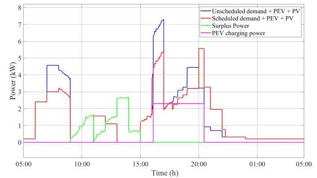
14. Else
 ( )
 15. = ( ),
 16. End if
 17. Elseif 2 is charging
 ℎ ( ) ℎ ℎ 
 18. = − (( ( ) − 0.08)/0.08) ∗ )
 19. Else
 ℎ ( ), ( )
 20. =0
 21. End if
 22. End for
 23. End if
 ℎ ( ), ( ),
 24. Return 2

5. Simulation and Result Discussion

 5.1 Scenario 1: Implementing smart scheduling strategy without V2H
 technique.
 The proposed scheduling strategy works based on real-time pricing (RTP), which is considered dynamic pricing.
Using the DR program, the customers receive price signals on an hour-ahead basis as the electricity price varies at
different time intervals of a day. Therefore, smart meters are used to receive the RTP signal from a utility and record
the current power consumption data of all household appliances and PEV charging during their operation times, and
then send them to the HEMS to manages and schedule the shiftable appliances. The simulation time is set at one day
(24 hours) with 1 second time step.

In order to evaluate the proposed scheduling strategy without implementing the V2H technique, two cases are
considered based on equipping the PV into the home due to its impact on the total household demand.

 5.1.1 Case 1: Demand + PEV
 In this case, there are some assumptions to be considered; I) The total household demand is the sum of all
household appliances consumption and random PEV charging. II) The PEV works under G2V mode only without
implementing PEV charging strategy in which the PEV battery charge from the power grid and it does not supply
power to the home. III) The user leaves the home by 09:00 and returns at 16:00 iv) Once the PEV is available, it starts
charging with the maximum power rate until the SOC reaches the maximum limit which is set to 80% in order to
avoid overcharging.

The daily energy consumption profile including all appliances’ consumption and PEV charging shown in Figure 6,

and the electricity price signal received from the power utility is shown in Figure 7. Two critical peak demand periods

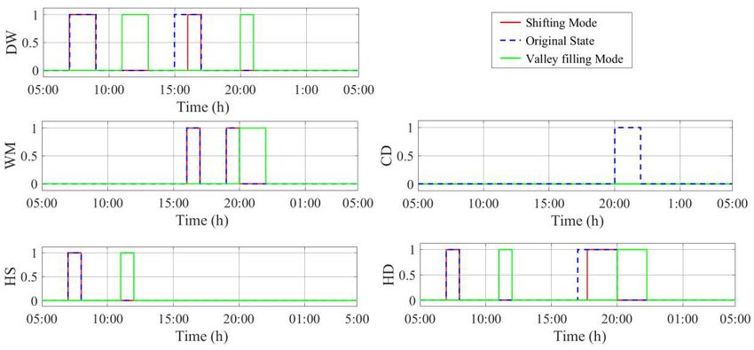
can be distinguished, which usually occur during morning and evening times when the electricity prices are higher.
Due to a decrease in user’s activities such as cooking, washing, cleaning, and watching TV, there is also off-peak
demand corresponding to a lower energy price.

 Figure 6 Energy demand profile (average limits in green lines)

 Figure 7 Electricity price

Based on the proposed approach discussed in section 4.1, HEMS detects Shifting, Valley filling and Do-nothing modes.
For example, the morning peak demand occurs during [07:00-09:00], where the total household demand is High and
the electricity price is Expensive, hence the Shifting mode should be applied according to the fuzzy rules shown in
Table 3. Based on algorithm 1, the total rated power of the operating times of all shiftable appliances is less than the
shifting required power. As a result, Dish Washer, Hair straightener and Hair Dryer appliances have been shifted as
shown in Figure 9. During the period [9:00-14:00], the proposed control algorithm detects Do-nothing mode as shown

in Figure 8 (a), since the total household demand is Low and the electricity price is Expensive. Consequently, the
operating time of the shiftable appliances maintains as it is. During the time [11:00-13:00], Valley Filling mode is
detected because the load profile is Low and the electricity price is Cheap. According to algorithm 1, the total rated
power of shifted appliances is more than the valley filling required power. As a result of this, HEMS switches on all

the shiftable appliances which have been shifted before. Based on this technique, Figure 8 (b) shows the final power
consumption profile of the household appliances over 24 hours.

 (a) (b)

 Figure 8 (a) scheduling output, (b) Power profile

 Figure 9 Operating status of shiftable appliances case 1

5.1.2 Case 2: Demand + PEV + PV
 In this case, it is assumed that the studied home is equipped with PEV, and PV. The same assumptions
regarding the PEV data mentioned in the previous case are applied here too. The PV produces power during the period
[08:00-19:00] as shown in Figure 10 (b) and supply to the home appliances when needed and store the surplus power

in a stationary battery. According to the proposed scheduling strategy, all scheduling actions are shown in Figure 10
(a)

 (a) (b)
 Figure 10 (a) scheduling output, (b) Power profile

For example, the total energy demand during [09:00-11:00] is Low and the electricity price is Expensive, hence the
Do-nothing mode is detected but as shown in fig, the PV-generated power is increasing from 480Wh to 1900Wh.
Therefore, in this period the demand is covered by the PV, and the surplus power shown in the green line is transferred
to the stationary battery for later use. During the period [11:00-13:00], valley filling mode is applied where shifted
appliances are turned on and consume all its power from the PV. It is noted that at 15:00 Do nothing mode is operating
due to the PV supplement which has changed the demand energy level from high to low as shown in fig, Therefore,
DW did not shift all its operating period compared to the previous case. The same scenario is applied for the HD at
17:00. As shown below in Figure 11

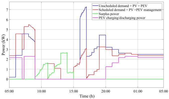
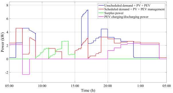
Figure 11 Operating status of shiftable appliances case 2

 5.2 Scenario 2: Smart scheduling strategy with V2H technique
 In this case, the electricity demand for each time-step in the household can be obtained from the home appliances,
PV generated power and PEV charging/discharging power. The PEV works under G2V and V2H operating modes in
which the PEV battery charge from the grid and supplies power to the home when needed according to the PEV
management strategy discussed in section 4.2. To demonstrate the performance of the proposed design, the initial
SOC of the PEV is set manually in different scenarios. Each scenario represents a critical limit of the SOC where the
proposed strategies must perform as expected to satisfy user comfort and fulfill utility requirements. In the following
cases, set at 09:00 and at 16:00.

 5.2.1 Case 1: the initial SOC is 80 %.
 According to the output of the PEV fuzzy control system, Figure 12 (a) shows the three possible actions;

Discharging (V2H), Charging, and Do nothing. Figure 12 (b) shows the SOC of PEV based on the action made while

Figure 13 shows the power demand profile before and after the proposed strategies. In this case, the initial SOC is set
as 80%. The EV supplied power to the household appliances (Discharging) for one hour during the first peak period
(high demand and expensive price) [07:00-08:00]. According to algorithm 2 lines 8-13, the discharging power rate
depends on the total rated power of demand. For example, when the total rated power of the demand is less than the
maximum discharging power the discharging power is set to the same value as the total rated power demand.
Otherwise, the discharging rated power will be set to the maximum value. Therefore, the discharging power rate during
[07:00-08:00] is set to maximum. The charging mode started during off-peak hours (low demand and cheap price)
from [20:00] and ended at [02:00] when the SOC reached 80%. The remaining time of the day, the PEV was outside

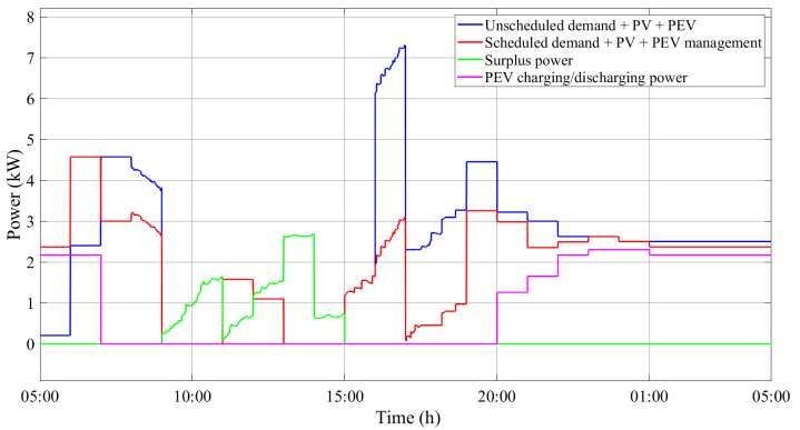
the home [09:00-16:00] or operated in “Do nothing” mode, where there was no need for “Charging” and
“Discharging” modes to maintain the capacity limits set using the equation (6).

 (a) (b)
 Figure 12 (a) PEV management fuzzy controller output, (b) PEV power and SOC%

 Figure 13 Power profile

 5.2.2 Case 2: the initial SOC is 60 %.
 In this case, Figure 15 shows the power demand profile before and after the proposed strategies under this

case scenario. Moreover, as shown in Figure 14 (b), the PEV started the day with 60% of SOC. During the first two
hours [05:00-07:00] when the electricity price and power demand are low, PEV started “Charging” mode according
to the fuzzy rules shown in Table 3. During the hours [07:00 – 09:00], the price is expensive, the SOC is high and the
scheduled demand is high, which resulted in operating with “Discharging” mode to supply power to the appliances
for only one hour [07:00-08:00]. Because the PV starts supplying power from 08:00, the total scheduled demand is
decreased hence the “Do nothing” mode is operating leaving almost 65% SOC at [09:00] when the user left the home.
At 16:00, the user arrived and plugged the vehicle in with 40% SOC while the total demand is low and the electricity
price is cheap. Therefore, “Do nothing” mode is activated avoiding charging with high cost. Then, the “Charging”
mode started again at [20:00] when the total scheduled demand is low and the electricity price is cheap. By the end of

the day, SOC was 80% to ensure that the user will start the next day with more stored energy in the PEV’s battery.
Compared to case 1, in Figure 14 (a) during the hour [06:00-07:00], the PEV is charging with low price in order to
store enough power to supply the household appliances.

 (a) (b)

 Figure 14 (a) PEV management fuzzy controller output, (b) PEV power and SOC%

 Figure 15 Power Profile

 5.2.3 Case 3: the initial SOC is 30 %.
 In Figure 16, with low initial SOC (30%), it can be noticed that there is no chance to supply power to the
appliances whatever the observed states. PEV started to operate on the “Charging” mode at [05:00] during off-peak
morning hours till [07:00]. This helped the user to leave the home with 40% of SOC and then he came back at [16:00]
with quite low SOC (less than 20%). Hence, the “Charging” mode started again until SOC reached 60%. again, a new
peak generated noticed in Figure 17 during the hour [06:00-07:00] where the PEV is charging with low price but in
this case, the PEV still has low SOC therefore it did not supply the household appliances. Finally, by the end of the
day, the SOC reached more than 60% hence, case 2 will be the case for the next day.

(a) (b)
 Figure 16 (a) PEV management fuzzy controller output, (b) PEV power and SOC%

 Figure 17 Power Profile

 5.2.4 Case 4: the initial SOC is 30 % and the target SOC at the departure
 time is 50%
 In this case, the same scenario of case 3 is applied with 50% SOC requested by the user at the departure time.
Therefore, the controller has calculated the time duration needed for the forced charging process in order to maintain
50% SOC at 09:00 using equation (8). As shown in Figure 18 (a) although the do-nothing mode is operating, at 07:20

the forced charging process has been applied. As shown in Figure 19, It can be noticed that before the forced charging
processes the PEV battery was charging during the period 05:00 – 07:00 where the charging power was calculated
using equation (2).

(a) (b)

 Figure 18 (a) PEV management fuzzy controller output, (b) PEV power and SOC %

 Figure 19 Power profile

Table 5 summarizes the cost of all mentioned scenarios. Where the total cost can be calculated as follow:

 ( ) = ∑ = ( ) ∗ ( ) (15)

In the first scenario case 1, with 30% initial SOC of the PEV battery, the total cost before applying the smart scheduling
strategy is 6.85. however, the total cost has been reduced by 2.33% with implementing the proposed scheduling
strategy. Moreover, it can be observed that the total cost reduction is 3.08% when the initial SOC of the PEV battery
is 80%. In addition, it is noted that the PV has contributed to more cost reduction compared to the 30% and 80% of
SOC in the first scenario by 7.29% and 10.14% respectively. In the second scenario, the charging/discharging strategy
contributes by 19.28% cost reduction when the initial SOC of the PEV is low (30%) while the cost reduction is 14.27%
when the initial SOC of the PEV is 80%.

Table 5 Total cost and cost reduction of all simulation cases

 Smart scheduling strategy PEV charging strategy
 Demand + PEV Demand + PEV + PV
 Initial Cost
 Cost Cost
 SOC% Before After Before After Before After reduction
 reduction reduction
 scheduling scheduling scheduling scheduling rate
 rate rate
 30% 6.852 6.692 2.33% 5.704 5.288 7.29% 5.288 4.268 19.28%
 60% 5.899 5.739 2.71% 4.751 4.335 8.75% 4.335 3.762 13.21%
 80% 5.183 5.023 3.08% 4.031 3.622 10.14% 3.622 3.105 14.27%

6. Conclusion
 In this paper, a smart scheduling strategy for smart home appliances assisted with the PEV energy management
strategy is presented. On one hand, the smart scheduling strategy aims to guarantee that the load profile does not
violate the grid-related requirements such as peak generation and satisfy the household needs by maintaining the same
amount of energy consumption with less cost by changing the operation period of shiftable appliances from peak hours
when energy prices are high to off-peak hours when energy prices are low. On the other hand, the PEV energy
management system is developed to coordinate the charging/discharging modes considering the travel needs of the
PEV owner by maintaining enough SOC before each trip. Both proposed strategies are developed using the fuzzy
logic system because it simplifies the overall implementation, leads to better performance, and lower time-consuming
as compared to other techniques. The simulation results show that the overall demand profile was smoothened, user
comfort has been satisfied and the cost of the total energy consumption was reduced by 19.28% and 14.27% in the
case of 30% and 80% initial SOC of the PEV, respectively. For more reliability and independence in future work,
further grid technical objectives will be considered, and reinforcement learning technique could be investigated
considering the PEV mobility.

7. Declarations

Ethical Approval

“Not applicable”.

Consent to participate

“Not applicable”.

Consent for publication

“Not applicable”.

Availability of data and materials

Data sharing is not applicable to this article as no datasets were generated or analysed during the current study.

Competing interests

"The authors declare that they have no competing interests".

Authors' contributions

KA created the model and the computational framework, as well as the data analysis. The implementation was
carried out by KA and FA. The computations were carried out by KA. The manuscript was written by KA and FA,
with contributions from all authors KA, FA and LS. The study was supervised by LS, who was also in charge of
overall direction and planning.

Funding

“Not applicable”.

 References
[1] H. J. Jabir, J. Teh, D. Ishak, and H. Abunima, “Impacts of demand-side management on electrical power
 systems: A review,” Energies, vol. 11, no. 5, pp. 1–19, 2018, doi: 10.3390/en11051050.

[2] N. G. Paterakis, O. Erdinç, and J. P. S. Catalão, “An overview of Demand Response : Key-elements and
 international experience,” Renew. Sustain. Energy Rev., vol. 69, no. September 2015, pp. 871–891, 2017, doi:
 10.1016/j.rser.2016.11.167.

[3] V. Durvasulu and T. M. Hansen, “Benefits of a demand response exchange participating in existing bulk-
 power markets,” Energies, vol. 11, no. 12, 2018, doi: 10.3390/en11123361.

[4] X. Hou, J. Wang, T. Huang, T. Wang, and P. Wang, “Smart Home Energy Management Optimization Method
 Considering Energy Storage and Electric Vehicle,” IEEE Access, vol. 7, pp. 144010–144020, 2019, doi:
 10.1109/ACCESS.2019.2944878.

[5] B. Cui, S. Wang, and X. Xue, “Effects and performance of a demand response strategy for active and passive
 building cold storage,” Energy Procedia, vol. 61, pp. 564–567, 2014, doi: 10.1016/j.egypro.2014.11.1171.

[6] B. Zhou et al., “Smart home energy management systems : Concept , con fi gurations , and scheduling

strategies,” vol. 61, pp. 30–40, 2016, doi: 10.1016/j.rser.2016.03.047.

[7] S. Aslam, N. Javaid, M. Asif, U. Iqbal, Z. Iqbal, and M. A. Sarwar, “A mixed integer linear programming
 based optimal home energy management scheme considering grid-connected microgrids,” 2018 14th Int.
 Wirel. Commun. Mob. Comput. Conf., pp. 993–998, 2018, doi: 10.1109/IWCMC.2018.8450462.

[8] C. H. Antunes, “A Mixed-integer Linear Programming Model for Optimal Management of Residential
 Electrical Loads under Dynamic Tariffs,” 2018.

[9] Z. Foroozandeh, S. Ramos, F. Lezama, Z. Vale, and R. L. Joench, “A Mixed Binary Linear Programming
 Model for Optimal Energy Management of Smart Buildings,” pp. 1–16, 2020.

[10] S. Resources, “An Optimized Home Energy Management System,” pp. 1–35, doi: 10.3390/en10040549.

[11] B. Lokeshgupta and S. Sivasubramani, “Cooperative game theory approach for multi- objective home energy
 management with renewable energy integration,” pp. 1–8, 2018, doi: 10.1049/iet-stg.2018.0094.

[12] R. N. and J. J., “Load Scheduling using Fuzzy Logic in a Home Energy Management System,” Int. J. Eng.
 Technol., vol. 10, no. 5, pp. 1263–1272, 2018, doi: 10.21817/ijet/2018/v10i5/181005013.

[13] C. V. Chandran, M. Basu, and K. Sunderland, “Comparative study between direct load control and fuzzy logic
 control based demand response,” Proc. - 2016 51st Int. Univ. Power Eng. Conf. UPEC 2016, vol. 2017-Janua,
 pp. 1–6, 2016, doi: 10.1109/UPEC.2016.8114090.

[14] M. M. Rahman, S. Hettiwatte, and S. Gyamfi, “An intelligent approach of achieving demand response by
 fuzzy logic based domestic load management,” 2014 Australas. Univ. Power Eng. Conf. AUPEC 2014 - Proc.,
 no. October, pp. 1–6, 2014, doi: 10.1109/AUPEC.2014.6966610.

[15] E. Fuzzy, L. Controller, and M. Systems, “Embedded Fuzzy Logic Controller and Wireless Communication
 for Home Energy,” 2018, doi: 10.3390/electronics7090189.

[16] R. Khalid, N. Javaid, M. H. Rahim, S. Aslam, and A. Sher, “Sustainable Computing : Informatics and Systems
 Fuzzy energy management controller and scheduler for smart homes,” Sustain. Comput. Informatics Syst.,
 vol. 21, pp. 103–118, 2019, doi: 10.1016/j.suscom.2018.11.010.

[17] F. Chekired, A. Mahrane, Z. Samara, M. Chikh, A. Guenounou, and A. Meflah, “Fuzzy logic energy
 management for a photovoltaic solar home,” Energy Procedia, vol. 134, pp. 723–730, 2017, doi:
 10.1016/j.egypro.2017.09.566.

[18] A. Verma, A. Asadi, K. Yang, and S. Tyagi, “A data-driven approach to identify households with plug-in
 electrical vehicles (PEVs),” Appl. Energy, vol. 160, pp. 71–79, 2015, doi: 10.1016/j.apenergy.2015.09.013.

[19] M. Denai, “Enhanced Electric Vehicle Integration in the UK Low-Voltage Networks With Distributed Phase
 Shifting Control,” IEEE Access, vol. 7, pp. 46796–46807, 2019, doi: 10.1109/ACCESS.2019.2909990.

[20] B. Storage, E. C. Reduction, and P. Demand, “Electric Vehicle ( EV ) in Home Energy Management to Reduce
 Daily Electricity Costs of Residential Customer,” vol. 77, no. October, pp. 559–565, 2018.

[21] M. S. A. Khan, K. M. Kadir, K. S. Mahmood, M. I. I. Alam, A. Kamal, and M. M. Al Bashir, “Technical
 investigation on V2G, S2V, and V2I for next generation smart city planning,” J. Electron. Sci. Technol., vol.
 17, no. 4, p. 100010, 2019, doi: 10.1016/j.jnlest.2020.100010.

[22] T. International, R. Energy, and A. Irena, “Electric Vehicles: Technology Brief”, 2017

[23] A. T. Radu, M. Eremia, and L. Toma, “Promoting battery energy storage systems to support electric vehicle
 charging strategies in smart grids,” 2017 Electr. Veh. Int. Conf. EV 2017, vol. 2017-Janua, pp. 1–6, 2017, doi:
 10.1109/EV.2017.8242092.

[24] M. Nour, S. M. Said, A. Ali, and C. Farkas, “Smart Charging of Electric Vehicles According to Electricity
 Price,” no. February, 2019, doi: 10.1109/ITCE.2019.8646425.

[25] S. Sachan, S. Deb, and S. N. Singh, “Different charging infrastructures along with smart charging strategies
 for electric vehicles,” Sustain. Cities Soc., vol. 60, no. May, p. 102238, 2020, doi: 10.1016/j.scs.2020.102238.

[26] Y. Chen, S. Member, J. M. Chang, and S. Member, “Fair Demand Response with Electric Vehicles for the
 Cloud Based Energy Management Service,” vol. 3053, no. c, pp. 1–11, 2016, doi:
 10.1109/TSG.2016.2609738.

[27] S. Khemakhem, M. Rekik, and L. Krichen, “Double layer home energy supervision strategies based on
 demand response and plug-in electric vehicle control for flattening power load curves in a smart grid,” Energy,
 vol. 167, pp. 312–324, 2019, doi: 10.1016/j.energy.2018.10.187.

[28] I. Serban, S. Céspedes, and S. Member, “Communication Requirements in Microgrids : A Practical Survey,”
 vol. 8, 2020.

[29] R. Hylsberg, J. Søren, and A. Mikkelsen, “Infrastructure for Intelligent Automation Services in the Smart
 Grid,” 2014, doi: 10.1007/s11277-014-1682-6.

[30] L. Xiao, G. Yao, S. Bu, and S. Member, “Pricing-Based Demand Response for a Smart Home With Various
 Types of Household Appliances Considering Customer Satisfaction,” IEEE Access, vol. 7, pp. 86463–86472,
 2019, doi: 10.1109/ACCESS.2019.2924110.

[31] M. Pipattanasomporn, M. Kuzlu, S. Rahman, and Y. Teklu, “Load Profiles of Selected Major Household
 Appliances and Their,” vol. 5, no. 2, pp. 742–750, 2014.

[32] Q. Xu and X. Jiao, “Research on a Demand Response Interactive Scheduling Model of Home Load Groups,”
 J. Electr. Eng. Technol., no. 0123456789, 2020, doi: 10.1007/s42835-020-00406-9.

[33] R. Bussar et al., “Battery energy storage for smart grid applications,” Assoc. Eur. Automot. Ind. Batter. Manuf.,

2013.

[34] B. University, “Electric Vehicle (EV).” https://batteryuniversity.com/learn/article/electric_vehicle_ev
 (accessed Oct. 22, 2020).

[35] P. Nayak and K. Rajashekara, “Single-stage Bi-directional Matrix Converter with Regenerative Flyback
 Clamp Circuit for EV Battery Charging,” pp. 1–6, 2019.

[36] Renewable, International Agency, Energy, INNOVATION OUTLOOK CHARGING FOR ELECTRIC, 2019