Preprint: Clip Art Rendering of Smooth Isosurfaces
←
→
Page content transcription
If your browser does not render page correctly, please read the page content below
1

Preprint: Clip Art Rendering of Smooth Isosurfaces
         Accepted pending revision for IEEE Transactions on Visualization and Computer Graphics
                                  3rd Revision, submitted January, 2007
                              Matei Stroila, Elmar Eisemann and John C. Hart, Member, IEEE

   Abstract— Clip art is a simplified illustration form consisting of
layered filled polygons or closed curves used to convey 3-D shape
information in a 2-D vector graphics format. This paper focuses
on the problem of direct conversion of smooth surfaces, ranging
from the free-form shapes of art and design to the mathematical
structures of geometry and topology, into a clip art form suitable
for illustration use in books, papers and presentations.
   We show how to represent silhouette, shadow, gleam and other
surface feature curves as the intersection of implicit surfaces,
and derive equations for their efficient interrogation via particle
chains. We further describe how to sort, orient, identify and fill
the closed regions that overlay to form clip art. We demonstrate
the results with numerous renderings used to illustrate the paper
itself.
   Index Terms— particle systems, non-photorealistic rendering,
line art drawing                                                            Fig. 1. An implicit Beethoven bust (left) converted into clip art consisting
                                                                            of layered, closed, 2-D curves (right) indicating silhouettes, shadows and
                                                                            highlights.
                         I. I NTRODUCTION
      OMPUTER GRAPHICS is largely the study of com-
C     putational tools for visual communication, which often
relies on rendering — the ability to display a computer
                                                                            layered filled polygons or closed curves that form the clip-
                                                                            art output. This vector output format eases the scaling and
representation of a geometric object. Photorealism focuses on               placement of figures in a document, and is significantly less
physical modeling and simulation but does not always lead to                memory-consumptive than raster images.
better shape recognition [22]. Non-photorealistic and artistic                 Our output appears similar to cartoon rendering which
rendering techniques instead utilize the knowledge of human                 typically alters the shading of a rendered polygonal mesh to
perception, long understood by artists and designers, to auto-              produce flat surfaces. Cartoon rendering often focuses on mesh
matically construct illustrations that convey an object’s shape,            shading, producing either a raster image or a 2-D polygon
often quite simply with minimal rendering primitives. Such                  soup of reshaded mesh triangles. In either case such cartoon
abstraction is furthermore an important tool for comprehension              shading produces larger output files than our clip art approach.
and memorization [27].                                                      Section II further compares this clip art approach to other NPR
   This paper focuses on a specific style of NPR called clip                methods.
art, by which we mean a small number of layered, filled                        Another alternative is to trace contours or feature lines in a
polygons or closed curves, as shown in Fig. 1. Such clip                    rendered image, which is simpler and supports a wider variety
art representations are commonly available in a wide variety                of models (anything that can be rendered). However, the
of authoring tools for articles, books and presentations. Clip              foreshortening inherit in any viewing projection can compress
art libraries are generated by designers specially trained to               large surface regions near the silhouette, leading to numerical
use this medium to convey the essence of a shape despite                    imprecision, raster artifacts and noise along the very feature
its minimal geometry. This paper focuses on automating this                 curves most important to effective illustration. As demon-
process to directly create clipart renderings from smooth free-             strated in Fig. 2, tracing contours in object space produces
form surfaces.                                                              watertight region boundaries whose resolution is limited only
   We generate clip art by sampling surface feature curves                  by the number of feature-curve samples used (which grows
in object space, connecting these samples into closed feature               linearly as the image resolution increases). Though we do not
curves, and projecting and ordering these curved into the 2-D               pursue this further here, these object space contours better
   Dept. of Computer Science, University of Illinois, Urbana-Champaign
                                                                            facilitate further output stylization than those extracted from
   M. Stroila is currently at NAVTEQ and can be contacted at                a rendered image.
matei.stroila@gmail.com                                                        We sample surface feature curves with a a surface-
   E. Eisemann is a student at ARTIS-GRAVIR/IMAG-INRIA and can be con-
tacted at elmar.eisemann@inrialpes.fr. ARTIS is a team of the GRAVIR/IMAG   constrained particle system [28]. Previous particle-based NPR
laboratory, a joint effort of CNRS, INRIA, INPG and UJF.                    approaches [13], [25] tracked each feature curve as surface-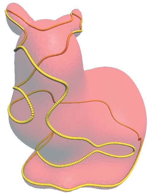
2
A. Smooth Surface Illustration
Vectorized Toon-Shading
Hertzmann and Zorin [17] also studied the illustration
of smooth surfaces, but instead of general isosurfaces they
applied a smooth interpolant to an input surface mesh that
cleverly caused the contour generator to avoid vertices that
lead to some degenerate cases they demonstrated. Elber [10]
Vectorization with our approach likewise relied on a polygonal approximation of a smooth
isosurface to construct an initial uniform distribution of points
that were projected onto the isosurface via gradient flow.
These points were then swept into strokes along the surface to
generate line-art textured renderings of the smooth isosurface.
Burns et al. [6] track silhouettes of volumetric isosurfaces,
capitalizing on the voxel grid’s fixed resolution for an efficient
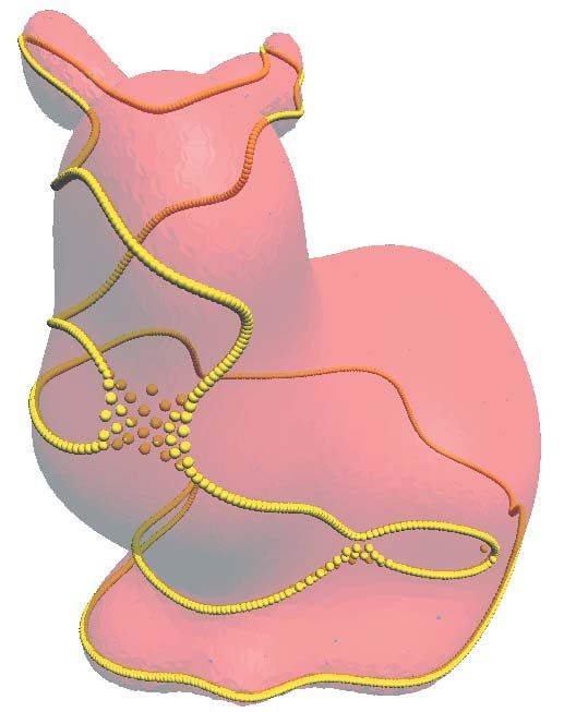
Fig. 2. Contouring a rendered image (left) can be inaccurate near the step size, and using a stochastic neighborhood test to detect
silhouette whereas tracking feature curves in 3-D (right) more accurately silhouettes. Our work focuses on the direct extraction of closed
tracks contours. silhouette and feature curves from a smooth implicit surface,
though some of our results are demonstrated on implicit
surfaces constructed from the embedding of a surface mesh,
surface intersection (SSI), using two simultaneous but in- using a B-spline space interpolant.
dependent particle-on-surface constraints. Section III shows
that these independent constraints can generate particles in
equilibria away from both surfaces, and devises a new two- B. Direct Isosurface Illustration
surface particle constraint that correctly samples these SSI
Bremer and Hughes [5] directly tracked the contour gener-
feature curves. While this constraint-based approach is not
ator of an implicit surface via predictor-corrector Euler inte-
guaranteed to accurately detect and trace all contours, it works
gration of its tangent vector (a so-called “marching” method),
well enough to produce illustrations.
seeded by intersecting a random interior ray to find the surface
Using this new SSI particle constraint, Section IV reviews which was then traversed in a random direction to find the sil-
how various surface feature curves including silhouettes, shad- houette. Foster et al. [13] similarly traced isosurface contours
ows1 , gleams and parabolic points can be represented as using seed points found by the surface constrained “floater”
the intersection of implicit surfaces. It also extends this SSI particles of Witkin and Heckbert [28]. Su and Hart [25]
approach to include suggestive contours, and introduces a reprogrammed these “floater” particles to adhere to silhouettes,
simpler suggestive contour approximation justified with visual by constraining them to both the implicit surface and the view-
comparison. tangency isosurface, but when computed independently, these
These feature curve particles connect to form closed chain dual constraints can counteract each other leading to errors.
loops which project to delineate view-plane polygonal regions. Section III derives the correct two-surface constraint.
Section V shows how to carefully manage the curve orientation
and visibility of these polygonal regions to produce the layered
filled polygons or closed curves that form the vector graphics C. Surface-Surface Intersection
format of clip art output.
As mentioned in the last paragraph, our surface illustra-
Section VI shows that the system runs fast enough to render
tions are built on the correct tracking of the intersection of
simple clip art (consisting of thousands of curve sample points)
two implicit surfaces. Surface-surface intersection is a classic
in real time, which allows the user to orient objects and po-
problem of computer-aided geometric design attacked with a
sition lighting to achieve an effective illustration. Section VII
wide array of approaches [18]. Because of the difficulty in their
concludes with ideas for further research.
surface navigation, implicit-implicit intersections are often
computed through space subdivision (a “lattice” approach).
For example, Suffern & Balsys [26] use interval subdivision
II. R ELATED W ORK
to extract and plot silhouette and other surface intersection
Our work focuses on the direct non-photorealistic rendering contours on implicit surfaces. Plantinga and Vegter [24]
of the isosurfaces of smooth (C3 ) functions by extracting use interval arithmetic to trace the contour generator with
various closed contour loops to generate layers of filled 2- a dynamic step size, thus guaranteing its correct topology.
D image curves. This work builds on the wealth of existing Our intersection contour tracking using chained dual-surface
approaches to NPR, many of which are summarized in surveys “floater” particles is more similar to a marching approach,
[1], [19]. though one whose sample points evolve in parallel instead of
in serial. In particular our particle tracking of contours is based
1 These shadow contours divide regions facing toward and away from a light
entirely on geometry and, unlike Plantinga and Vegter [24],
source. We do not yet consider the detection and generation of cast shadow is not guaranteed to find and properly trace all contours,
contours. especially near visual events.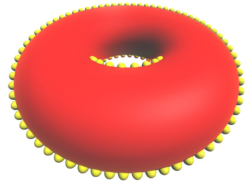
3

D. Dynamic Surface Illustration                                          Substituting the velocities computed from (6) into (3) and
   Many techniques for real-time extraction of silhouettes            (4), we obtain the system
recompute their projection from scratch [23]. Kalnins et                              λi |∇Fi |2 + µi ∇FiT ∇Gi       = CFi (Vi ),                  (7)
al. [20] studied the coherence of stylized silhouettes, using
                                                                                      λi ∇GTi ∇Fi + µi |∇Gi |2       = CGi (Vi ).                  (8)
the previous silhouettes to seed a new extraction of the next
frame’s silhouettes. The particles we use to track the silhouette        Then, we compute the Lagrangian multipliers λi and µi from
work similarly for dynamic surfaces or views. We do not               the above system of equations and plug them in the following
yet explore the detection and correction of contour topology,         velocity update equations, which rewrite (6) as
and rely on the purely geometric algorithm used to connect
particles into a closed contour to reconnect contours after a                                 vi = Vi − λi ∇Fi − µi ∇Gi .                          (9)
visual event.
                                                                         Working out the details, it follows that if the two surfaces
                                                                      are not tangent at xi then the linear system for the Lagrange
                    III. C URVE A DHESION                             multipliers has solutions
   In this section, we present our extension of the surface
                                                                                  CGi (Vi )   CFi (Vi )

                                                                                                            ∇FiT ∇Gi       |∇Fi |2

adhesion behavior of Witkin and Heckbert [28] to a curve              λi =                  −            /             −             ,
                                                                                  |∇Gi |2     ∇FiT ∇Gi       |∇Gi |2     ∇FiT ∇Gi
adhesion behavior.
                                                                                                            ∇FiT ∇Gi      |∇Gi |2

   The condition that n moving particles, xi (t) lie on the                       CFi (Vi )   CGi (Vi )
                                                                      µi =                  −            /            −              .
intersection curve of two smooth surfaces defined implicitly                       |∇Fi |2    ∇FiT ∇Gi       |∇Fi |2     ∇FiT ∇Gi
by F = 0 and G = 0 is given by                                        An important remark is that the Lagrange multipliers λi and µi
                   Fi (t) ≡ F(xi (t)) = 0,                     (1)    are not just CFi (Vi )/|∇Fi |2 and CGi (Vi )/|∇Gi |2 . These would
                                                                      be the expressions obtained by solving separately the two sur-
                   Gi (t) ≡ G(xi (t)) = 0.                     (2)    faces’ adhesions, which lack the interacting terms containing
Differentiating with respect to time yields 2n linear dynamic         the dot product ∇FiT ∇Gi . Therefore, by only superposing two
constraint equations                                                  surface adhesion solutions, the particles would not converge
                                                                      to the correct curve. Figure 3 depicts this situation. Realize in
               CFi (vi ) ≡ ∇FiT vi + φ Fi    = 0,              (3)    particular that the surface in this example is relatively simple
               CGi (vi ) ≡ ∇GTi vi + φ Gi    = 0.              (4)    and smooth.

of the particle velocities vi = dxi /dt, where the additional                                Independent                          Interdependent
                                                                                             Surface                              Surface
“feedback” terms (scaled by constant φ ) are added for nu-                                   Adhesion                             Adhesion
merical stability to bring particles xi back to the zero surface
if they stray.
   In fact it is precisely this feedback term that causes particles
to lie off the intersection curve (between curves) when using
two independent particle-on-surface dynamic constraints. A
dynamic constraint removes forces that would move a particle
off its current isovalue contour, so a particle’s implicit surface
function value remains constant, though not necessarily the
desired value of zero in this case. These “feedback” terms
are spring-like penalty constraints that nudge particles to a
desired isovalue, whereas the dynamic constraint keeps them
                                                                      Fig. 3. Particles separately constrained to two surfaces (here the shown
there. Particles can thus fall between isovalue contours when         implicit surface and the implied shadow-contour surface) can find off-surface
opposing feedback terms cancel.                                       equalibria (left). A two-surface simultaneous dynamic constraint contain
   Particle curve adhesion is then achieved by solving the            additional terms such that particles correctly adhere only to the surface-surface
                                                                      intersection curve (right).
following constrained optimization problem
                (                                          )
                   1 n           2 CFi (vi ) = 0
  v = arg min        ∑ |vi − Vi | CGi (vi ) = 0 , ∀i = 1, n . (5)
                   2 i=1                                                                     IV. F EATURE C ONTOURS

where Vi are the desired particle velocities, set to a mutual            Many of the feature curves on implicit surfaces used in
particle repulsion force to evenly distribute the particles [28].     computer graphics can be expressed as the intersection of the
  Following the Lagrange multipliers method, the gradient of          implicit surface with a second implicit surface. For example,
the objective function with respect to the minimizing variables       an implicit shape’s silhouette in object space (more formally
{vi }, should be equal to a linear combination of the gradients       its contour generator) is the curve found at the intersection of
of the constrain functions                                            the shape’s implicit surface and the implicit surface formed by
                                                                      the dot product of the shape function’s gradient and the view
                 vi − Vi + λi ∇Fi + µi ∇Gi = 0.                (6)    vector. This section defines such implicit intersection curves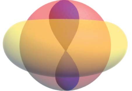
4

 for silhouettes, shadows, parabolic points, suggestive contours                     surface with the shadow surface, which is as well implicitly
 and gleams.                                                                         defined as the zeroset of
     We start with a few basic definitions and notations. Let
 x ∈ R3 be the position vector of an arbitrary point located                                                   Fshad = ∇F(r)T~vl .                         (12)
 on the implicit surface S = F −1 (0), for a smooth function                         Such shadow curves are demonstrated in Figure 5.
 F : R3 → R. We assume that 0 is a regular value of F, so that
 the surface S is smooth. We also assume that the function F
 has C3 differentiability (the third order partial derivatives exist
 and are continuous).
     In order to support both orthographic and perspective view
 projections, and both point and directional light sources, we let
 c = (c1 , c2 , c3 , ch ) = (~c, ch ) be the homogeneous coordinates of
 the position vector of the camera (the viewpoint), and let l =
 (~l, lh ) be the homogeneous position vector of the light source.
 We denote by ~vc = ~c − ch x the view direction vector, and by
~vl = ~l − lh x the light direction vector.

A. Silhouette Contours
  A point x ∈ S is on the contour generator of a smooth
surface if the view vector is tangent to the surface at x, or
equivalently, it is orthogonal to the surface normal at x. For                       Fig. 5. Shadow and silhouette contours combined with shading on Moai
                                                                                     (left) and Horse (right).
an implicit surface F −1 (0), the surface normal direction is the
support line of the gradient ∇F(x). The contour generator can
                                                                                        The shadow curve definition can also be extended to a
hence be regarded as the curve given by the intersection of the
                                                                                     family of isophote curves defined by different fixed acute
implicit surface with the silhouette surface, which is defined
                                                                                     angles between the surface normal and the light vector. This
implicitly as the zeroset of
                                                                                     can be seen as a quantized Lambertian reflectance, as shown
                             Fsil = ∇F(x)T~vc .                             (10)     in Fig. 6.
The normal of the silhouette surface is given by the gradient
       ∇(Fsil ) = ∇(∇F(x)T~vc ) = H F(x)~vc − ch ∇F(x)                      (11)
where H F(x) is the Hessian matrix of F at x. A silhouette
surface for a torus is demonstrated in Figure 4.

                                                                                     Fig. 6. An interpolated volumetric Stanford bunny, displayed as clip art
                                                                                     consisting of isophotes of constant diffuse reflectance (left) stacked from
                                                                                     individual isophote layers (right).

Fig. 4. The apparent contour (yellow) of the view along vector v (left) is the
projection of the contour generator (yellow) shown from a side-view (right) at
the intersection of the implicit surface F = 0 (red) and the (implicit) silhouette   C. Gleams and Reflection Lines
surface ∇F · v = 0 (green).
                                                                                        Gleams (or more precisely specular highlights) are intended
                                                                                     to be the reflections of light sources on the surface of an object,
                                                                                     though graphics tends to use a reflectance approximation
B. Shadow Contours and Isophotes                                                     which yields round specular lobes from a point light source.
   The shadow contour of a free-form object is defined as the                        Specular reflections are an important visual cue as they reveal
set of points on the object surface where the surface normal                         details in a given shape, and designers commonly use reflection
is perpendicular to the vector from the light source. As such,                       lines resulting from the reflection of light strips to assess the
we have to use the light position vector instead of the camera                       aesthetic quality of a shape, e.g. a car body.
position vector in all the formulas of the previous section.                            For rendering such gleams and reflection lines in “clip art”
   As in the contour generator case, the shadow can be                               style illustrations, we describe the specular contour as the
regarded as the curve defined by the intersection of the implicit                    boundary of the regions where the strength of the specular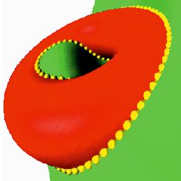
5
reflection of light lies above a certain threshold. Following When viewed from one of its tangent directions, the contour
Blinn’s specular reflectance formulation [3], let the halfway generator forms a cusp and the apparent contour stops in an
vector be h = ~vl /||~vl || +~vc /||~vc || and n be the normal vector ending contour. Consequently, here the radial curvature is
to the surface at x. Then, the specular contour is the set of zero implying that the apparent contours and the suggestive
points on the surface where h and n form a fixed angle α contours meet. Suggestive contours and apparent contours line
up with geometric tangent continuity in the image plane.
Cspec = {x ∈ S|∠(h, n) = α}. (13)
The specular contour is then the intersection of the implicit
surface with the specular surface, with the latter defined as the
zeroset of the function
Fspec = ∇F(x)T h − arccos(α)k∇F(x)kkhk. (14)
Figure 7 demonstrates these specular contours.
Fig. 8. Suggestive contours meet the visible contour tangentially, extending
it to provide additional surface cues. The right suggestive contour (red, right)
occurs where radial curvature is zero. The left suggestive contour (blue, left)
approximates and simplifies radial curvature by not projecting the view vector
onto the surface tangent plane. (A right “blue” curve and left “red” curve have
been removed for illustration).
Although in general the radial curvature is defined only
at the surface’s points, for implicit surfaces, kr (x) can be
regarded as a real function over three-space. Hence, the sug-
gestive contour can be determined by intersecting the implicit
surface with the radial curvature zeroset, restricting the result
Fig. 7. Specularities convey important shape information in flat shaded areas. to points where the w-directional derivative of kr is positive.
The sketchy appearance of the teddy (left) is still apparent in the clip art. The The application of this definition of suggestive contours to
bull (right) contains lots of details that are faithfully transmitted, nevertheless
the cornes have been smoothed as they would represent singularities.
implicit surface particle dynamics is costly. The gradient of
radial curvature is quite complex,
T T w) H F∇F
T
∇kr (x) = 2w|w|H4Fw w − 2 (∇F ~vc )(∇F |∇F| 4 +
D. Suggestive Contours T T
(∇F w)(H F~vc −∇F)+(∇F ~vc ) H Fw
+
|∇F| 2
DeCarlo et al. [9] extended the apparent contour (the visible
1 3 i j
projection of the contour generator) to include additional |w|2 ∂·,i, j Fw w − (16)
shape cue feature curves called suggestive contours. These ((H Fw)T ∇F)(H F~vc −∇F)+(∇F T ~vc ) H F H Fw
2 −
|∇F|2
suggestive contours are built on the concept of radial curvature (∇F T ~vc )((H Fw)T ∇F) H F∇F
2 H Fw + 4 .
as described by Koenderink [21]. The radial curvature at a |∇F|4
point x is the normal curvature of the surface in the direction
We instead present a different definition for suggestive
given by the projection of the view vector, ~vc , onto the tangent
contours that is simpler with similar visual results. In particular
plane at x. We denote this projection vector by w. The radial
the contours still align with the ending contours. In fact for
curvature is view dependent and undefined whenever ~vc is
any curve on the surface that crosses a cusp, its projection has
parallel to n.
a tangent that aligns with the tangent of the apparent contour
For an implicit surface, the radial curvature at the point x
at the intersection point [9]. The only exception occurs when
is
1 T the curve locally projects to a point, that is to say, the tangent
kr (x) = w H F(x)w. (15)
|w|2 of the space curve aligns with the view direction.
Instead of applying the Hessian to the projection of the view
The suggestive contour is the set of points on the surface at
vector onto the tangent plane, w, we apply it directly to the
which the radial curvature kr is 0, and the directional derivative
view vector. We construct a simpler suggestive contour surface
of kr in the direction of w is positive. Thus, at a point of
as the zeroset of
the suggestive contour, w points in one of the asymptotic
directions of the surface (zero curvature directions). Fsug (x) =~vTc H F(x)~vc (17)
The set of points on the surface at which the radial curvature
kr is 0 forms a set of closed loops on the surface. These loops but only display its portions where
are cut at the points where the view vector is tangent to the ∇Fsug (x)T~vc > 0 (18)
surface.
The apparent contour is defined as the visible portions (which could be construed as a half-space whose boundary
of the contour generator projected onto the image plane. forms yet a third implicit surface).6
The gradient of this newly defined implicit function takes
the much simpler form (shown componentwise)
3 i j
∂k Fsug (x) = ∑(∂k,i, j F(x)vc vc ) − 2(H F(x)~
vc )k . (19)
i, j
The similarity to the original definition also comes from the
fact that in the ending contour the two curves actually coincide Fig. 11. A surface of parabolic points defined as the zeroset of an implicit
because the view direction lies in the tangent plane and Gaussian curvature formula that for the torus is a sphere surrounding an
thus the missing projection has no influence. These simpler hourglass (left). Only the sphere intersects the torus, yielding two circles
(right).
suggestive contours are demonstrated in Figures 9 and 10.
Fig. 9. Algebraic hollow cube (left) with suggestive contours (middle, dotted) Fig. 12. Silhouette (black) and parabolic contours (red) on the hollow cube
which are segments of our simplified radial curvature contours (right). (left) and squash (right).
V. C ONSTRUCTING C LIP A RT
The clip art construction process, diagrammed in Fig. 14
consists of converting a shape specification using implicit
surfaces into a depth-ordered list of layered closed filled curves
in a format that can be displayed by any of a variety of
vector graphics renderers. Our approach to clip art construc-
tion relies on the Witkin-Heckbert method of sampling and
displaying an implicitly defined shape using self-organizing
particles constrained to the implicit surface [28]. We use a fully
programmable version of this framework [25] to implement
new behaviors to interrogate the feature curves needed to
convert implicit surfaces into clip art closed loops.
Fig. 10. Kitty without (left) and with suggestive contours (middle) generated We begin with an implementation of “floater” particles [28],
from simplified radial curvature contours (right). altered to sample space curves instead of surfaces. One of these
alterations replaces the surface adhesion behavior that keeps
particles on an implicit surface with the surface-intersection
E. Parabolic Contours curve adhesion behavior described in Section III. We also alter
The parabolic contours consist in surface points where the the particle repulsion behavior, ordinarily used to distribute
Gaussian curvature is zero. They can also be regarded as particles evenly over a surface, to achieve a force equilibrium
intersections of implicit surfaces using the Gaussian curvature using only two “curve” neighbors instead of six “surface”
formula for an implicit surface, which is defined over the entire neighbors when particles settle on the surface. As is standard,
embedding space [14] we also use a grid spatial data structure to accelerate particle
neighborhood queries [16].
∇F(x)T H F(x)∗ ∇F(x)
kG (x) = (20) In addition to simple repulsion, these curve particles need
k∇F(x)k4 to properly connect with their neighbors to form closed loops.
where H F(x)∗ is the adjoint of the Hessian matrix (the adjoint
of a matrix is the transpose of its cofactor matrix). Because we
are interested in its zeroset, we can focus on the numerator of
this expression which makes the calculation simpler and more
stable.
The parabolic contours contain the critical points of the
silhouette and shadow contours and so indicate where they
change topology under different viewing/lighting conditions.
Figure 13 demonstrates such a change in the shadow contours Fig. 13. Shadow contours on the squash passing through a critical point.
of an illuminated squash. The critical points of the shadow contours are also parabolic points.7
Adhesion behavior leads Chain particles to loops Classify region type at Shade final contour-defined
particles to contour curves Compute planar graph and visibility triangulation samples layered vectorial output
Fig. 14. We convert an implicit surface specified by a function into clipart specified by layered filled 2-D polygons by using particles to find surface feature
curves and determining how those closed spacecurves should be layered and shaded when projected to 2-D.
Previous implementations simply connect a particle with its particles surrounding a cusp to precisely determine the change
two nearest neighbors which works well most of the time but in quantitative invisibility. These extensions are necessary
can prove unstable in some situations such as sharp turns. because visibility cannot be propagated in the exact same way
We instead rely on the differential geometry of the curve, as it is for polygonal meshes. (This is why Burns et al. [6]
constructing a tangent vector from the cross product of the two rely on a cast ray per silhouette voxel.)
implicit surfaces whose intersection defines the curve. We use We seek to decompose the curve into segments of constant
this information to better predict a particle’s two neighbors, quantitative invisibility. In the case of closed loops, this is
which have to lie in different half-spaces, as defined by the guaranteed if we do not cross behind other silhouette edges
tangent. or the radial curvature does not change sign [17].
Given one or more closed space curves, we then need to For each loop in the arrangement graph mentioned earlier,
project them into simple closed curves in the image plane. We we apply the following procedure. First, we pick randomly
first project the space curves into possibly overlapping image one of its edges and assign a relative QI of zero. (We don’t
curves. These intersections must be transverse and we use know the actual quantitative invisibility yet, but we need a
perturbations to avoid tangential crossings when they occur. reference). Then, we propagate the QI along the loop edge by
We then use the CGAL computational geometry library [4] edge, changing it only when we encounter a vertex of higher
to construct an arrangement of intersecting curves [12]. This degree (global occlusion) or when its radial curvature changes
arrangement is a planar graph where each vertex corresponds sign (local occlusion).
to an intersection point of the projected curves, and in our For global occlusion, we can assume we look down the z-
case, each edge maintains an ordered list of particles on axis and that the vertex in the planar graph corresponds to a
the corresponding curve segment connecting the intersection point P on a contour loop for which we want to propagate
points. This arrangement allows the overlapping space curves visibility. All global intersections that have an influence on
to be decomposed into simple closed image curves joined at the QI have to be situated between P and the viewpoint.
the intersection points. If the curve overlapping P is ordinary (no cusp), then the
The remainder of this section focuses on the ordering and QI changes by two (intuitively, due to the front- and back-
shading of these simple closed image curves, to produce a facing part of the interloping surface). If the normal of the
direct clip art depiction of the implicit surface. interloping silhouette agrees with the orientation of our current
loop, we decrement the QI by two, otherwise we increment.
A. Visibility In practice this normal comes from the two closest particles
Given a collection of closed image curves depicting closed on the occluding silhouette.
space curves on an implicit surface, we first need to identify For a global occlusion where the occluding silhouette con-
the visible segments of the image curves. For particles other tains a cusp that overlaps our current loop, the QI remains
than those on the contour generator, we use the surface unchanged, unless the current loop is tangent to the cusp, and
normal to cheaply identify back facing curve segments. For in this rare case the QI changes by two.
the remaining curve segments, we determine the visibility Local occlusions occur at cusps, where the radial curvature
of an individual particle by casting a single ray intersected changes sign. We use the depth of the sample particles near the
against the implicit surface. Visibility can also be efficiently cusp to determine its effect on the QI. Let zi and zi+1 be the
propagated along the curve segment. depths of the two particles (ordered from the loop orientation)
We propagate visibility along the contour generator using on each side of the cusp. If zi < zi+1 then we increment
Appel’s hidden line algorithm [2] originally derived for polyg- QI, otherwise we decrement it. This relation between radial
onal meshes and more robustly updated for smooth surfaces curvature and the effect of a cusp on QI can be proved as
[23], parameteric surfaces [11], and implicit surfaces [5]. We follows. Intuitively, within a neighborhood of a silhouette
similarly extend Appel’s algorithm to implicit surfaces and point, the surface is locally above or below the view rays
this section shows how to march along the particle chains and depending on the radial curvature sign. This restriction of the
use their relationship with the implicit surface’s differential surface flips at a cusp which signals an increase or decrease
geometry to overcome otherwise difficult cases. In particular, in depth complexity.
we use the depth order and radial curvatures of the two More rigorously, since the surface is smooth there exists a8
surface neighborhood B of the cusp diffeomorphic to R2 that
maps the contour generator to the x-axis. Let C be any smooth
surface curve in this neighborhood that (1) connects a point
N on the near silhouette branch in front of the cusp and a
point F on the far silhouette branch behind cusp, (2) maps via
the diffeomorphism to the y > 0 region except at its endpoints
where y = 0 (C does not cross the contour generator), and
(3) there exist surface neighborhoods BN , BF ⊂ B about N and
F whose intersections with the radial planes at those points
coincides with C.
Restating Lemma 2.3 of Elber and Cohen [11] a surface
curve that does not intersect the contour generator has constant Fig. 15. Contour curves and visibility information are insufficient to deduce
local QI. Such is the case for the interior of C. shading. The dashed lines indicate two possible surfaces that share the same
Assume κr > 0 at N and let point P ∈ C ∩ BN . If P = N contour lines (silhouette and shadow) but one hides the small sphere whereas
the other does not.
(the only silhouette point in C ∩ BN ) its (relative) QI = 0 (it
is visible) locally in this neighborhood. For points close to N
the local QI = 1 because of κr > 0. Locally the curve remains apparent contour and the visible surface contours such that
inside of the face of the local arrangement, which implies that their interiors lie on the left. Shadowed areas are then indicated
the QI remains constant in the interior of C (by the above by resulting cycles (shadow in the bottom right of Figure
lemma). Locally we find that the QI of F equals the QI of 16). In the presence of occluding contours this approach fails
points nearby in C ∩ BF (this time due to κr < 0). We conclude (shadow in the middle of the same figure).
that the local QI for F has to be 1. The proof for κr < 0 follows
similarly.
Once we have obtained the relative QI for the curve, we
ground it to an absolute QI through a single ray query. We
choose to perform this ray query on a point on the segment
with the largest (relative) QI.
B. Shading
While the apparent contour outlines the object, we still
need to fill in these outlines to visually disambiguate regions Fig. 16. Correctly oriented silhouette and shadow contours form closed
especially among complex combinations of specularities and cycles in the planar graph as long as no occluding contours appear.
shadows. While one could output triangles in a vector graphics
format, they increase the size of the output with non intuitive Still each face of the planar graph of visible contours can
components. be categorized (e.g. gleam, illuminated, shadowed or void).
We instead seek to output clip art consisting of layers of We can determine the category by casting a single eye ray
filled closed polygons defined by projections of the visible that pierces each region, though we find multiple piercing eye
portions of various surface contours. This section focuses on rays help avoid occasional errors due to numerical instabilities
identifying these regions and constructing consistently oriented in tight regions such as near the apparent contour. These region
planar polygons. piercing rays should not pass too closely to region boundaries
Given a consistently oriented contour generator (based on and we explored several approaches to choose these rays:
the tangent) on a smooth surface, one can correctly fill its random sampling, skeletal points and the barycenters of a
apparent contour using its winding number. This simplicity constrained Delaunay triangulation. The latter best balanced
does not extend to the filling of shadows, specularities and speed and accuracy, and consistently classified over 95% of
other closed surface regions. Figure 15 demonstrates a scene the regions in our experiments.
where complete knowledge of all contour information does
not help in identifying the proper fill regions. The grey dashed
VI. R ESULTS
lines indicate two different configurations that lead to identical
visible silhouette and shadow contours. We implemented our particle-based contour illustration
As long as no occluding contours occur, the contours’ ori- system using the Wickbert surface and particles system
entation plus the particles’ visibility suffice to shade shadows library (http://www.uiuc.edu/goto/wickbert), a
(and specularities) correctly. One problem that arises is, that user-extensible open-source cross-platform C++ library [25]
surface curves align with silhouettes making the construction based on the surface constrained particle systems of Witkin
of the planar graph more difficult. Nevertheless these intersec- and Heckbert [28]. Wickbert implements a framework for pro-
tions occur at visibility events. For a correct planar graph we gramming particle systems using building-block interchange-
can connect the last visible particle to the closest silhouette able attributes, behaviors and shaders. Curve adhesion was
and rely on ray tracing in the case of doubt. We orient the implemented as a new particle behavior, and new particle9
shaders were devised to organize and display closed polyline needed to correctly fill the closed contour output. This is
curves. followed by a less expensive constrainted Delauney triangula-
Using this system, we can manipulate (zoom, rotate) quartic tion (CDT). Both operations exceed the time expected of an
surfaces in real-time using up to 4000 particles for feature interactive system, so we rely on the particle-based contour
contours rendering, on an Intel T2500 2.0GHz processor with display for interactive posing, lighting and manipulation, and
2.00GB of memory. compute the planar map and CDT when exporting to a portable
vector graphics format (SVG).
Timings Table (System: Intel T2500 2.0GHz, 2.00 GB of RAM) The resulting clipart generated by the the system was used
Particles Clip art
Model Cont. # Implicit Visibility Repulsion Adhesion Total
Plan.
CDT
to illustrate the various sections of the paper. The clip art
Map
Type Particles
ms ms ms ms ms s s displayed is polygonal except for Figures 1 and 6, where we
Sil. 531 1.09 4.49 1.54 0.09 7.21
Hollow
Shad. 529 1.08 2.10 1.48 0.10 4.76
replaced the polygons with closed filled spline curves. Splines
Cube 1.92 0.13
(Algebraic)
Spec. 246 0.50 2.40 0.44 0.06 3.40 are smoother and can more compactly represent curved regions
Sugg. 390 1.01 3.31 0.94 0.98 6.24
Beethoven
Sil. 1010 33.00 41.00 4.97 0.19 79.16 than could polygons, but care must be taken when fitting to
Shad. 1197 43.53 21.36 6.45 0.19 71.53
Bust
Spec. 1119 40.09 39.88 5.72 0.12 85.81
6.92 0.42 avoid introducing overlap between neighboring regions.
(Volumetric)
Sugg. 1024
Sil. 225
31.10
40.00
31.74
106.56
5.39
0.41
40.37
0.05
108.60
147.02
Our vector clip art resolution depends on the number of
Beethoven
Bust (RBF,
Shad. 306 62.51 94.65 0.86 0.09 158.11
1.20 0.11 particles used, and particle sampling density can be curva-
Spec. 204 39.28 91.55 0.41 0.06 131.30
504 ctrs.)
Sugg. 493 94.98 254.86 1.86 103.62 455.32 ture dependent, whereas raster processing operates at a fixed
resolution. Our particle approach renders an implicit directly,
TABLE I efficiently focusing its effort on contour generation whereas
T IMING BREAKDOWN PER TASK ACROSS ALGEBRAIC , VOLUMETRIC AND raster processing must sample the entire visible surface, throw-
RBF IMPLICIT SURFACES . ing away most of the interior per-pixel results. Finally the
resulting curves do not suffer from occlusion problems and
are three dimensional loops, which is of particular importance
Table I shows the timings for three different models and for the usability for NPR stylized line drawings [15].
respectively three different implicit representations: algebraic
(quartic), cubic B-spline interpolation of a 323 -grid volume VII. C ONCLUSIONS AND F UTURE W ORK
and radial basis function interpolation of 504 scattered data In this paper we presented a new particle-based method
points. for the direct conversion of smooth surfaces (represented as
The Implicit column measures the total time per screen- implicit surfaces) into clip art (vectorial graphics with closed
update iteration to evaluate the implicit surface function and curves). We developed a new particle behavior designed to
its derivative. Direct evaluation of RBF’s remains slow, though track curves at the intersection of two implicit surfaces, and
speedups exist via the fast multipole method [7], [8]. However, showed how to represent various feature curves as such,
spline interpolation of RBF’s sampled in a voxel grid results in including a new, more efficient version of suggestive contours.
a smooth surfaces that supports a much faster evaluation. The The result is a useful tool for generating clip art for illus-
local coefficients for the splines are recalculated per particle tration of free-form shapes and visualization of the differential
per frame. Storing these coefficients per particle could further geometry of smooth curves and surfaces. Because our system
accelerate performance at the expense of a larger memory is built on the Witkin-Heckbert surface particles [28], an
footprint. additional feature is that it supports the direct manipulation of
For proof of concept we computed a ray-cast visibility per- the displayed shape by dragging the particles in the displayed
particle, measured in the Visibility column. While this was contours. Other sculpting modifications are also possible.
the most expensive per-particle operation, it can be reduced Although this paper’s work focuses on the creation of
by propagating quantitative invisibility. static clip art, the particle system inheres a certain temporal
The Repulsion timing indicate the total time per screen- coherence. Several algorithms use the old silhouettes as a
update iteration to compute inter-particle repulsion. We used a seed for detecting the new ones [6], [23]. In our approach
simple O(n2 ) algorithm to find distances between each particle silhouettes are moved directly by particles which keep their
and every neighbor, which sufficed for the 1-D contours used relative positions as long as no critical point is encountered.
for illustration. We would use an O(n)-time grid locality This is a result of the optimization scheme implemented in
acceleration structure for depiction with surface particles. the silhouette adhesion behavior that finds the silhouette as a
The Adhesion column likewise computes the surface- one dimensional variety. For slow view changes, the particles
surface intersection adhesion described in Sec. III, which maintain the loop structure once it is established. We did not
is inexpensive except for suggestive contours, because of notice changes in the particles relative neighbors as long as
the significantly greate amount of arithmetic required. This smooth silhouettes are concerned.
additional arithmetic includes some numerical finite difference Several opportunities for future work exist:
approximations of higher derivatives that were not imple- • Simple particle tracing is not guaranteed to accurately
mented by default in our implicit surface system, which require trace the contour, nor to find all contours. The addition
many additional implicit surface function evaluations. of interval or Lipschitz methods based on analysis of the
These per-particle computations are nevertheless dominated implicit surface’s defining function could provide such a
by the significantly more expensive planar map construction, guarantee [24].10
• Our shadow contours separate regions facing toward and [18] J. Hosche and D. Lasser. Fundamentals of Computer Aided Geometric
away from a light source. We trace rays to determine Design. AK Peters, 1993.
[19] Tobias Isenberg, Bert Freudenberg, Nick Halper, Stefan Schlechtweg,
contour visibility and one could use the same approach and Thomas Strothotte. A Developer’s Guide to Silhouette Algorithms
to add cast-shadow contours. for Polygonal Models. IEEE CG&A, 23(4):28–37, 2003.
• We plan to investigate contour control through camera [20] Robert D. Kalnins, Philip L. Davidson, Lee Markosian, and Adam
Finkelstein. Coherent stylized silhouettes. (Proc. SIGGRAPH) ACM
motion and shape deformation as a tool for automatically TOG, 22(3):856–861, 2003.
enhancing the communication ability of this display form. [21] J J Koenderink. What does the occluding contour tell us about solid
• More complicated shading patterns, like gradients, would shape? Perception, 13(3):321–30, 1984.
[22] Jan J. Koenderink. Solid shape. MIT Press, 1990.
be simple to integrate in our output for improved visual [23] Lee Markosian, Michael A. Kowalski, Daniel Goldstein, Samuel J.
effects. Trychin, John F. Hughes, and Lubomir D. Bourdev. Real-time non-
• We currently only manually determine that splines fit to photorealistic rendering. In Proc. SIGGRAPH, pages 415–420, 1997.
[24] Simon Plantinga and Gert Vegter. Computing contour generators of
the contours do not overlap significantly. evolving implicit surfaces. ACM Trans. Graph., 25(4):1243–1280, 2006.
• We are interested in the correct contour topology main- [25] Wen Y. Su and John C. Hart. A programmable particle system frame-
tenance across a visual event. work for shape modeling. In SMI ’05: Proceedings of the International
Conference on Shape Modeling and Applications 2005 (SMI’ 05), pages
• The clip-art approach traces three dimensional loops that 114–123, Washington, DC, USA, 2005. IEEE Computer Society.
allow the integration of our system into, for example, the [26] Kevin G. Suffern and Ronald J. Balsys. Rendering the intersections of
framework of Grabli et al. [15] where the user can create implicit surfaces. IEEE CG&A, 23(5):70–77, 2003.
[27] Holger Winnemoeller, Sven C. Olsen, and Bruce Gooch. Real-time
an unlimited variety of line drawings based on a scripted video abstraction. ACM TOG, 25(3):1221–1226, 2006.
shading language. [28] Andrew P. Witkin and Paul S. Heckbert. Using particles to sample and
control implicit surfaces. In Proc. SIGGRAPH, pages 269–277, 1994.
In other words, we have achieved the goal of producing
portable vector graphics clip art from smooth implicit surfaces,
but in the process opened up many new directions in need of
further investigation.
R EFERENCES
[1] Wang Ao-yu, Tang Min, and Dong Jin-xiang. A survey of silhouette
detection techniques for non-photorealistic rendering. In 3rd Intl. Conf.
on Image and Graphics (ICIG’04), pages 434–437, 2004.
[2] Arthur Appel. The notion of quantitative invisibility and the machine
rendering of solids. In Proc. 22nd Natl. Conf., pages 387–393, 1967.
[3] James F. Blinn. Models of light reflection for computer synthesized
pictures. Proc. SIGGRAPH, Computer Graphics, 11(2):307–316, 1977.
[4] CGAL Editorial Board. CGAL-3.2 User and Reference Manual, 2006.
[5] David J. Bremer and John F. Hughes. Rapid approximate silhouette
rendering of implicit surfaces. In Proc. Implicit Surfaces, pages 155–
164, 1998.
[6] Michael Burns, Janek Klawe, Szymon Rusinkiewicz, Adam Finkelstein,
and Doug DeCarlo. Line drawings from volume data. In Proc.
SIGGRAPH, pages 512–518, 2005.
[7] J. C. Carr, R. K. Beatson, J. B. Cherrie, T. J. Mitchell, W. R. Fright,
B. C. McCallum, and T. R. Evans. Reconstruction and representation
of 3d objects with radial basis functions. In Proc. SIGGRAPH, pages
67–76, 2001.
[8] J. C. Carr, R. K. Beatson, B. C. McCallum, W. R. Fright, T. J. McLennan,
and T. J. Mitchell. Smooth surface reconstruction from noisy range data.
In Proc. GRAPHITE, pages 119–ff, 2003.
[9] Doug DeCarlo, Adam Finkelstein, Szymon Rusinkiewicz, and Anthony
Santella. Suggestive contours for conveying shape. ACM TOG,
22(3):848–855, 2003.
[10] Gershon Elber. Line art illustrations of parametric and implicit forms.
IEEE TVCG, 4(1):71–81, 1998.
[11] Gershon Elber and Elaine Cohen. Hidden curve removal for free form
surfaces. In Proc. SIGGRAPH, pages 95–104, 1990.
[12] Eyal Flato, Dan Halperin, Iddo Hanniel, Oren Nechushtan, and Eti
Ezra. The design and implementation of panar maps in cgal. J. Exp.
Algorithmics, 5:13, 2000.
[13] K. Foster, P. Jepp, B. Wyvill, M. C. Sousa, C. Galbraith, and J. A. Jorge.
Pen-and-ink for BlobTree implicit models. CG Forum, 24(3):267, 2005.
[14] Ron Goldman. Curvature formulas for implicit curves and surfaces.
CAGD, 22(7):632–658, 2005.
[15] Stéphane Grabli, Emmanuel Turquin, Frédo Durand, and François Sil-
lion. Programmable style for npr line drawing. In Rendering Techniques
(Proc. EGSR), pages 33–44. ACM Press, 2004.
[16] Paul Heckbert. Fast surface particle repulsion. Tech Report CMU-CS-
97-130, 1997.
[17] Aaron Hertzmann and Denis Zorin. Illustrating smooth surfaces. In
Proc. SIGGRAPH, pages 517–526, 2000.You can also read