Predicting Crime Using Twitter and Kernel Density Estimation
←
→
Page content transcription
If your browser does not render page correctly, please read the page content below
Predicting Crime Using Twitter and Kernel Density
                            Estimation

                                   Matthew S. Gerbera,∗
a
    Department of Systems and Information Engineering, University of Virginia, P.O. Box
           400747 Charlottesville, Virginia 22904-4747, United States of America

Abstract

Twitter is used extensively in the United States as well as globally, creat-
ing many opportunities to augment decision support systems with Twitter-
driven predictive analytics. Twitter is an ideal data source for decision
support: its users, who number in the millions, publicly discuss events, emo-
tions, and innumerable other topics; its content is authored and distributed
in real time at no charge; and individual messages (also known as tweets)
are often tagged with precise spatial and temporal coordinates. This article
presents research investigating the use of spatiotemporally tagged tweets for
crime prediction. We use Twitter-specific linguistic analysis and statistical
topic modeling to automatically identify discussion topics across a major
city in the United States. We then incorporate these topics into a crime
prediction model and show that, for 19 of the 25 crime types we studied,
the addition of Twitter data improves crime prediction performance versus
a standard approach based on kernel density estimation. We identify a num-
ber of performance bottlenecks that could impact the use of Twitter in an
actual decision support system. We also point out important areas of future
work for this research, including deeper semantic analysis of message con-

     ∗
         Email address: msg8u@virginia.edu; Tel.: 1+ 434 924 5397; Fax: 1+ 434 982 2972

Preprint submitted to Decision Support Systems                          January 14, 2014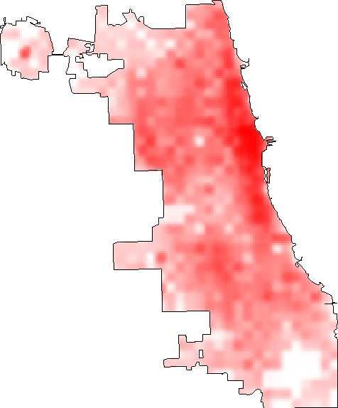
tent, temporal modeling, and incorporation of auxiliary data sources. This
research has implications specifically for criminal justice decision makers in
charge of resource allocation for crime prevention. More generally, this re-
search has implications for decision makers concerned with geographic spaces
occupied by Twitter-using individuals.
Keywords: Crime prediction, Twitter, Topic modeling, Density estimation

1. Introduction

   Twitter currently serves approximately 140 million worldwide users post-
ing a combined 340 million messages (or tweets) per day [1]. Within the
United States in 2012, 15% of online adults used the Twitter service and
8% did so on a typical day, with the latter number quadrupling since late
2010 [2]. The service’s extensive use, both in the United States as well as
globally, creates many opportunities to augment decision support systems
with Twitter-driven predictive analytics. Recent research has shown that
tweets can be used to predict various large-scale events like elections [3],
infectious disease outbreaks [4], and national revolutions [5]. The essential
hypothesis is that the location, timing, and content of tweets are informative
with regard to future events.
   Motivated by these prior studies, this article presents research answering
the following question: can we use the tweets posted by residents in a major
U.S. city to predict local criminal activity? This is an important question
because tweets are public information and they are easy to obtain via the
official Twitter service. Combined with Twitter’s widespread use around
the globe, an affirmative answer to this question could have implications
for a large population of criminal justice decision makers. For example,
improved crime prediction performance could allow such decision makers to

                                      2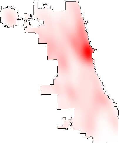
more efficiently allocate police patrols and officer time, which are expensive
and thus scarce for many jurisdictions.
   However, there are many challenges to using Twitter as an information
source for crime prediction. Tweets are notorious for (un)intentional mis-
spellings, on-the-fly word invention, symbol use, and syntactic structures
that often defy even the simplest computational treatments (e.g., word
boundary identification) [6]. To make matters worse, Twitter imposes a
140-character limit on the length of each tweet, encouraging the use of these
and other message shortening devices. Lastly, we are interested in predict-
ing crime at a city-block resolution or finer, and it is not clear how tweets
should be aggregated to support such analyses (prior work has investigated
broader resolutions, for example, at the city or country levels). These fac-
tors conspire to produce a data source that is simultaneously attractive –
owing to its real time, personalized content – but also difficult to process.
Thus, despite recent advances in all stages of the automatic text processing
pipeline (e.g., word boundary identification through semantic analysis) as
well as advances in crime prediction techniques (e.g., hot-spot mapping),
the answer to our primary research question has remained unclear.
   We pursued three objectives: (1) quantify the crime prediction gains
achieved by adding Twitter-derived information to a standard crime pre-
diction approach based on kernel density estimation (KDE), (2) identify
existing text processing tools and associated parameterizations that can
be employed effectively in the analysis of tweets for the purpose of crime
prediction, and (3) identify performance bottlenecks that most affect the
Twitter-based crime prediction approach. Our results indicate progress to-
ward each objective. We have achieved crime prediction performance gains
across 19 of the 25 different crime types in our study using a novel applica-

                                      3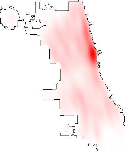
tion of statistical language processing and spatial modeling. In doing so, we
have identified a small number of major performance bottlenecks, solutions
to which would benefit future work in this area.
   The rest of this article is structured as follows: in Section 2, we survey
recent work on using Twitter data for predictive analytics. In Section 3,
we describe our datasets and how we obtained them. In Section 4, we
present our analytic approach for Twitter-based crime prediction, which we
evaluate in Section 5. In Section 6, we discuss our results and the runtime
characteristics of our approach. We conclude, in Section 7, with a summary
of our contributions and pointers toward future work in this area.

2. Related Work

2.1. Crime prediction

   Hot-spot maps are a traditional method of analyzing and visualizing
the distribution of crimes across space and time [7]. Relevant techniques
include kernel density estimation (KDE), which fits a two-dimensional spa-
tial probability density function to a historical crime record. This approach
allows the analyst to rapidly visualize and identify areas with historically
high crime concentrations. Future crimes often occur in the vicinity of past
crimes, making hot-spot maps a valuable crime prediction tool. More ad-
vanced techniques like self-exciting point process models also capture the
spatiotemporal clustering of criminal events [8]. These techniques are useful
but carry specific limitations. First, they are locally descriptive, meaning
that a hot-spot model for one geographic area cannot be used to characterize
a different geographic area. Second, they require historical crime data for
the area of interest, meaning they cannot be constructed for areas that lack

                                     4
such data. Third, they do not consider the rich social media landscape of
an area when analyzing crime patterns.
Researchers have addressed the first two limitations of hot-spot maps by
projecting the criminal point process into a feature space that describes each
point in terms of its proximity to, for example, local roadways and police
headquarters [9]. This space is then modeled using simple techniques such
as generalized additive models or logistic regression. The benefits of this
approach are clear: it can simultaneously consider a wide variety of historical
and spatial variables when making predictions; furthermore, predictions can
be made for geographic areas that lack historical crime records, so long as the
areas are associated with the requisite spatial information (e.g., locations of
roadways and police headquarters). The third limitation of traditional hot-
spot maps – the lack of consideration for social media – has been partially
addressed by models discussed in the following section.
2.2. Prediction via Social Media
In a forthcoming survey of social-media-based predictive modeling, Kalam-
pokis et al. identify seven application areas represented by 52 published
articles [10]. As shown, researchers have attempted to use social media to
predict or detect disease outbreaks [11], election results [12], macroeconomic
processes (including crime) [13], box office performance of movies [14], nat-
ural phenomena such as earthquakes [15], product sales [16], and financial
markets [17]. A primary difference between nearly all of these studies and
the present research concerns spatial resolution. Whereas processes like dis-
ease outbreaks and election results can be addressed at a spatial resolution
that covers an entire city with a single prediction, criminal processes can
vary dramatically between individual city blocks. The work by Wang et al.
5comes closest to the present research by using tweets drawn from local news
agencies [13]. The authors found preliminary evidence that such tweets
can be used to predict hit-and-run vehicular accidents and breaking-and-
entering crimes; however, their study did not address several key aspects
of social-media-based crime prediction. First, they used tweets solely from
hand-selected news agencies. These tweets, being written by professional
journalists, were relatively easy to process using current text analysis tech-
niques; however, this was done at the expense of ignoring hundreds of thou-
sands of potentially important messages. Second, the tweets used by Wang
et al. were not associated with GPS location information, which is often
attached to Twitter messages and indicates the user’s location when post-
ing the message. Thus, the authors were unable to explore deeper issues
concerning the geographic origin of Twitter messages and the correlation
between message origin and criminal processes. Third, the authors only in-
vestigated two of the many crime types tracked by police organizations, and
they did not compare their models with traditional hot-spot maps.
The present research addresses all limitations discussed above. We com-
bine historical crime records with Twitter data harvested from all available
Twitter users in the geographic area of interest. We address some of the
difficult textual issues described previously (e.g., symbols and nonstandard
vocabulary) using statistical language processing techniques, and we take full
advantage of GPS location information embedded in many tweets. Further-
more, we demonstrate the performance of our approach on a comprehensive
set of 25 crime types, and we compare our results with those obtained using
standard hot-spot mapping techniques.
6Figure 1: Number of tweets collected daily between January 1, 2013 and March 31, 2013.
The sharp spike on day 34 coincided with the United States Super Bowl. The three large
drops resulted from a failure in our data collection software on those days.
3. Data Collection
Chicago, Illinois ranks third in the United States in population (2.7
million), second in the categories of total murders, robberies, aggravated
assaults, property crimes, and burglaries, and first in total motor vehicle
thefts (January - June, 2012 [18]). In addition to its large population and
high crime rates, Chicago maintains a rich data portal containing, among
other things, a complete listing of crimes documented by the Chicago Police
Department.1 Using the Data Portal, we collected information on all crimes
documented between January 1, 2013 and March 31, 2013 (n = 60, 876).
Each crime record in our subset contained a timestamp of occurrence, lat-
itude/longitude coordinates of the crime at the city-block level, and one of
27 types (e.g., ASSAULT and THEFT). Table 1 shows the frequency of each
crime type in our subset.
1
City of Chicago Data Portal: https://data.cityofchicago.org
7Crime type Frequency (%)
THEFT 12,498 (20.53%)
BATTERY 10,222 (16.79%)
NARCOTICS 7,948 (13.06%)
CRIMINAL DAMAGE 5,517 (9.06%)
OTHER OFFENSE 4,183 (6.87%)
BURGLARY 3,600 (5.91%)
MOTOR VEHICLE THEFT 3,430 (5.63%)
ASSAULT 3,374 (5.54%)
DECEPTIVE PRACTICE 2,671 (4.39%)
ROBBERY 2,333 (3.83%)
CRIMINAL TRESPASS 1,745 (2.87%)
WEAPONS VIOLATION 635 (1.04%)
OFFENSE INVOLVING CHILDREN 593 (0.97%)
PUBLIC PEACE VIOLATION 583 (0.96%)
PROSTITUTION 418 (0.69%)
CRIM SEXUAL ASSAULT 264 (0.43%)
INTERFERENCE WITH PUBLIC OFFICER 244 (0.40%)
SEX OFFENSE 207 (0.34%)
LIQUOR LAW VIOLATION 121 (0.20%)
ARSON 79 (0.13%)
HOMICIDE 68 (0.11%)
KIDNAPPING 58 (0.10%)
GAMBLING 27 (0.04%)
STALKING 26 (0.04%)
INTIMIDATION 25 (0.04%)
OBSCENITY* 5 (0.01%)
NON-CRIMINAL* 2 (0.00%)
Total 60,876
Table 1: Frequency of crime types in Chicago documented between January 1, 2013 and
March 31, 2013. We excluded asterisked crimes from our study due to infrequency.
8Figure 2: KDE for GPS-tagged Tweets that originated within the city limits of Chicago,
Illinois between January 1, 2013 and March 31, 2013.
During the same time period, we also collected tweets tagged with GPS
coordinates falling within the city limits of Chicago, Illinois (n = 1, 528, 184).
We did this using the official Twitter Streaming API, defining a collection
bounding box with coordinates [-87.94011,41.64454] (lower-left corner) and
[-87.52413,42.02303] (upper-right corner). Figure 1 shows a time series of
the tweets collected during this period and Figure 2 shows a graphical KDE
of the tweets within the city limits of Chicago. As shown in Figure 2, most
GPS-tagged tweets are posted in the downtown area of Chicago.
94. Analytic Approach
To predict the occurrence of crime type T , we first defined a one-month
training window (January 1, 2013 – January 31, 2013). We then put down
labeled points (latitude/longitude pairs) across the city limits of Chicago.
These points came from two sources: (1) from the locations of known crimes
of type T within the training window (these points received a label T ), and
(2) from a grid of evenly spaced points at 200-meter intervals, not coinciding
with points from the first set (these points received a label NONE ). Using
all points, we trained a binary classifier with the following general form:
P r(Labelp = T |f1 (p), f2 (p), ..., fn (p)) = F (f1 (p), f2 (p), ..., fn (p)) (1)
In words, Equation 1 says that the probability of a crime of type T oc-
curring at a spatial point p equals some function F of the the n features
f1 (p), f2 (p), ..., fn (p) used to characterize p. We set F to be the logistic
function, leaving only the fi (p) features to be specified. In the next section,
we present feature f1 (p), which quantifies the historical crime density at
point p. Next, in Section 4.2, we present features f2 (p), ..., fn (p), which are
derived from Twitter messages posted by users in the spatial vicinity of p.
In Section 4.3, we present the model in full mathematical detail and explain
how we produced threat surfaces from the point estimates of threat.
4.1. Historical Crime Density: Feature f1 (p)
To quantify the historical density of crime type T at a point p, we set
f1 (p) to be the KDE at p:
P
1 X ||p − pj ||
f1 (p) = k(p, h) = K (2)
Ph h
j=1
10Figure 3: Neighborhood boundaries for computing tweet-based topics. We only used the
green neighborhoods (i.e., those within the city boundary) in our analysis.
In Equation 2, p is the point at which a density estimate is needed, h is
a parameter – known as the bandwidth – that controls the smoothness of
the density estimate, P is the total number of crimes of type T that oc-
curred during the training window, j indexes a single crime location from
the training window, K is a density function (we used the standard normal
density function), || · || is the Euclidean norm, and pj is the location of crime
j. We used the ks package within the R statistical software environment
to estimate k(p, h), and we used the default plug-in bandwidth estimator
(Hpi) with a dscalar pilot to obtain an optimal value for h. This standard
approach is widely used by crime analysts to estimate crime densities [7].
11Figure 4: Plate notation for LDA, the parameters of which are as follows: β is the hy-
perparameter for a Dirichlet distribution, from which the multinomial word distribution
φ(z) is drawn (1 ≤ z ≤ T ), T is the number of topics to model, α is the hyperparameter
for a Dirichlet distribution, from which the multinomial topic distribution θ(d) is drawn
(1 ≤ d ≤ D), D is the number of documents, z is a draw from θ(d) that identifies topic φ(z) ,
from which an observed word w is drawn. z and w are drawn Nd times independently.
4.2. Information from Twitter Messages: Features f2 , ..., fn
The primary contribution of this article is an exploration of Equation
1 for n > 1. That is, the novelty of this research lies in the combina-
tion of the standard kernel density estimate f1 (p) with additional features
f2 (p), ..., fn (p) that describe point p using Twitter content. Intuitively, one
can think of each fi (p) (for i > 1) as representing the importance of topic
i − 1 in the discussion that is transpiring among Twitter users in the spatial
neighborhood of p, with the total number of topics being n−1 (n is analogous
to k in k-means clustering, and we describe our approach for determining
its value in Section 5). We defined spatial neighborhoods in Chicago by
12laying down evenly spaced cells 1000 meters on each side. Figure 3 shows
the resulting neighborhood boundaries.
Given the neighborhoods defined above, the problem reduces to estimat-
ing the n−1 topic importance values for each neighborhood given the tweets
posted by users in each neighborhood. We used latent Dirichlet allocation
(LDA) for this purpose [19]. LDA is a generative probabilistic model of tex-
tual content that identifies coherent topics of discussion within document
collections. Figure 4 shows the traditional plate notation for LDA, and we
summarize the inputs and outputs below:
Documents: a collection of D textual documents with word boundaries.
Number of topics (T ): number of topics to model.
Using these inputs, the topic modeling process automatically infers optimal
settings for the following multinomial distributions:
Word distribution of topics (φ(z) ): the probability that each word be-
longs to (or defines) a topic z.
Topic distribution of documents (θ (d) ): the probability that each topic
belongs to (or defines) a document d.
Returning to Chicago and Equation 1, imagine compiling into a single
“document” all tweets posted during the training window within a single
neighborhood (see Figure 3). The map of Chicago then defines a collection
of such documents, and the topic modeling process estimates the strength of
each topic in each neighborhood – precisely what we need for our crime pre-
diction model. For example, in the neighborhood covering Chicago O’Hare
Airport, the strongest topic (with probability 0.34) contains the following
words:
13(3) flight, plane, gate, terminal, airport, airlines, delayed, american, ...
This is an intuitive result, since people often post tweets about traveling
while in an airport. Thus, for any point p falling into this neighborhood,
there exists a feature fi (p) = 0.34. The same point p is also associated with
the other T − 1 topic probabilities, producing the full set of topic features
{f2 (p), ..., fi (p) = 0.34, ..., fn (p)} for point p. Points in other areas of the
city will also have a value for fi (the “airport topic”), but this value will
generally be much lower since people in such areas will be less focused on
discussing airports and travel.
LDA topic modeling is completely unsupervised, requiring no human
effort to define topics or identify topic probabilities within neighborhoods.
Similar to unsupervised clustering, topics do not have textual labels. Above,
we labeled fi the “airport topic” for explanation purposes only – such labels
do not exist in our models. LDA also does not capture word order, making
each topic an unordered set of words. For our purposes, the key output of
LDA is the probability of each topic in each neighborhood. We hypothe-
sized that these probabilities would add information to f1 (p) (the historical
density) by injecting personalized descriptions from people’s everyday lives
into the model. Before showing the final model formulation and describing
its application, we provide additional implementation details describing how
we transformed raw tweets into the topic probabilities discussed above.
Implementing Topic Modeling for Tweets. Twitter is an inherently chal-
lenging source of textual information for reasons discussed earlier. Thus,
deep semantic analysis of tweets via traditional methods [20] is unlikely to
work well. Such methods suffer dramatic performance degradations when
switching from their training domain of newswire text to the relatively clean
14domain of general written English [21]. We eschewed deep semantic analy-
sis in favor of shallower analysis via topic modeling; however, we were still
confronted with the problems of word boundary detection and filtering out
irrelevant words (e.g., “the” and other so-called stop words). We addressed
these problems using the Twitter-specific tokenizer and part-of-speech tag-
ger developed by Owoputi et al. [22]. We processed each Tweet using this
software, and we retained all tokens marked with one of the following syn-
tactic categories:
common noun, pronoun, proper noun, nominal + possessive,
proper noun + possessive, verb, adjective, adverb, interjection,
hashtag*, emoticon*, nominal + verbal, proper noun + verbal,
existential ‘there’ + verbal
The list of retained syntactic categories is typical for filtering out stop words,
with the exception of the asterisked categories, which are unique to the so-
cial media domain. It is particularly important to use appropriate tokeniza-
tion for emoticons (e.g., “:)”), which would probably be treated as separate
tokens by a traditional tokenizer but carry important semantic content de-
scribing the user’s emotional state.
Once the tweets had been tokenized and filtered, we applied the MALLET
toolkit [23], which outputs the following probabilities:
P r(t|r) 1 ≤ t ≤ T = #topics
1 ≤ r ≤ R = #neighborhoods (4)
In words, Equation 4 denotes the proportion of the discussion within neigh-
borhood r that is devoted to topic t. Each of the R neighborhoods is de-
scribed in terms of its T topic probabilities, as discussed previously. A full
15description of the topic modeling algorithm is beyond the scope of this ar-
ticle, and we refer the interested reader to the seminal presentation [19] as
well as the official MALLET documentation [23].
4.3. Full Model Formulation and Application
The full form of our crime prediction model (Equation 1) for crime type
T , including coefficients, is defined as follows:
1
P r(Labelp = T |f1 (p), f2 (p), ..., fn (p)) =
n
(5)
Y
− β 0 +
βi fi (p)
1+e i=1
For i = 1, fi (p) equals the KDE k(p, h). For i > 1, fi (p) equals P r(i − 1|r)
from Equation 4, where r is the unique topic neighborhood that spatially
contains p. Recall that, during training, we have a set of points that are
labeled with the crime type T and a set of points that are labeled as NONE.
Thus, building the binary logistic regression model in Equation 5 can proceed
in the standard way once the density estimates and topic modeling outputs
are obtained.
For any model trained according to Equation 5, we sought predictions
for crimes of type T for the first day following the training period. We
obtained these predictions by evaluating Equation 5 at spatial points across
the prediction area. The set of prediction points included those obtained by
evenly spacing points at 200-meter intervals across the prediction area. We
also added to the set of prediction points all points where crimes of type
T occurred during the training window. We added these points to force
higher-resolution predictions in areas where we had observed more crime in
the past. In any case, a prediction point was simply a latitude-longitude
pair containing no ground-truth information about future crime.
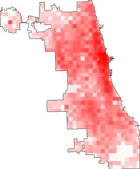
16(a) Predicted threat surface using only the (b) Predicted threat surface using the
KDE feature. KDE feature and the Twitter features.
Figure 5: Threat surfaces without (5a) and with (5b) Twitter topics.
For a prediction point p, we obtained feature value f1 (p) by inspect-
ing the density of crime T observed in the 31 days prior. We obtained
feature values f2 (p), ..., fn (p) by inspecting the topic modeling output for
tweets observed in the 31 days prior within the neighborhood covering p.
At this point, the model had already been trained and the coefficients βi
were known, so estimating the probability of crime type T at point p was
simply a matter of plugging in the feature values and calculating the result.
Note that this only produced point estimates of threat across the prediction
area. Since an individual point does not cover any geographic space, it was
necessary to translate the point estimates into surface estimates. To do this,
we simply recovered the 200-meter by 200-meter squares formed by the pre-
diction points spaced at 200-meter intervals and averaged the predictions in
17Figure 6: Spatially interpolated surface derived from Figure 5b according to Equation 6.
.
each square to calculate the threat for each square.
Figure 5a shows a threat surface produced by using only the KDE fea-
ture f1 (p), and Figure 5b shows a threat surface produced by adding 100
Twitter topic features f2 (p), ..., f101 (p) to the KDE. The former appears to
be smooth, since it comprises 200-meter threat squares. The latter also uses
200-meter threat squares, but any two points residing in the same 1000-
meter by 1000-meter topic neighborhood will have identical topic-based fea-
ture values. Thus, most of the topic neighborhoods in Figure 5b appear to be
uniformly colored. They are not, however, as can be seen in the downtown
Chicago area:2 note the graded threat levels within many of the downtown
topic neighborhoods in Figure 5b. Such gradations are produced by changes
18in the KDE feature.
Intuitively, the boundary between a safe neighborhood and a danger-
ous neighborhood in Figure 5b should not be crisp, at least not under our
neighborhood definition, which does not correlate with physical barriers that
might induce such a boundary. To operationalize this intuition, we applied
distance-weighted spatial interpolation to each prediction point p in the
topic-based models as follows:
|N (p,W )|
X W − D(p, ni )
P rI (Labelp = T, W ) = ∗ P r(Labelni = T )
|N (p,W )|
i=1 X
W − D(p, nj )
j=1
(6)
In Equation 6, P rI is the probability interpolation function, W is a window-
ing parameter of, for example 500 meters, N (p, W ) is the set of p’s neighbors
within a distance of W (this set includes p itself), D(p, ni ) is the straight-
line distance between p and one of its neighbors ni , and P r(Labelni = T )
is the non-interpolated probability given in Equation 5. Thus, the spatially
interpolated probability at point p is the weighted average of its neighbors’
probabilities (including p itself), and the weights are inversely proportional
to the distance between p and its neighbors. Figure 6 shows the visual result
of applying this smoothing operation to the threat surface in Figure 5b. In
the following section, we present a formal evaluation of various parameteri-
zations of the models described above.
2
The downtown Chicago area is the one that features most prominently in Figure 5a.
195. Evaluation and Results
For each crime type T , we compared the model using only the KDE fea-
ture f1 (p) to a model combining f1 (p) with features f2 (p), ..., fn (p) derived
from Twitter topics. We used MALLET to identify topic probabilities, con-
figured with 5000 Gibbs sampling iterations and an optimization interval
(how often to reestimate the α and β hyperparameters, see Figure 4) of 10,
but otherwise used the default MALLET parameters. We used LibLinear
[24] to estimate coefficients within the logistic regression model. To counter
the effects of class imbalance (there are far more negative points than pos-
N
itive points), we set LibLinear’s C parameter to P, with N and P being
the counts of negative and positive points in the training set, respectively.
Model execution entailed (1) training the model on a 31-day window for
crime type T , (2) making T predictions for the first day following the train-
ing window, and (3) sliding one day into the future and repeating. This
mirrors a practical setup where a new prediction for T is run each day.
We evaluated the performance of each day’s prediction using surveillance
plots, an example of which is shown in Figure 7. A surveillance plot mea-
sures the percentage of true T crimes during the prediction window (y-axis)
that occur within the x% most threatened area according to the model’s
prediction for T . The surveillance plot in Figure 7 says that, if one were
to monitor the top 20% most threatened area according to the prediction
for T , one would observe approximately 45% of T crimes. We produced
scalar summaries for surveillance curves by calculating the total area under
the curve (AUC). Better prediction performance is indicated by curves that
approach the upper-left corner of the plot area or, equivalently, by curves
with higher AUC scores. An optimal prediction sorts the 200-meter pre-
201.0
0.8
% incidents captured
0.4 0.6
Aggregated (AUC=0.7211)
0.2
0.0
0.0 0.2 0.4 0.6 0.8 1.0
% area surveilled
Figure 7: Example surveillance plot showing the number of true crimes captured (y-axis)
in the x% most threatened area according to the model’s prediction. AUC indicates total
area under the surveillance curve.
diction squares in descending order of how many future crimes they will
contain. This property makes surveillance plots appropriate for decision
makers, who must allocate scarce resources (e.g., police patrols) across the
geographic space. Lastly, because each model execution produced a series
of surveillance plots for crime type T , one for each prediction day, we aggre-
gated the plots to measure a model’s overall performance. For example, to
compute a model’s aggregate y-value for crime type T at an x-value of 5%,
we first summed the number of true T crimes occurring in the top 5% most
threatened area for each prediction day. We then divided that sum by the
21total number of true T crimes occurring across all prediction days. Doing
this for each possible x-value produced an aggregate curve and aggregate
AUC score, which we report in this article.
Evaluation proceeded in two phases. First, for each crime type, we op-
timized the number of topics and smoothing window in the Twitter-based
model during a development phase. We experimented with 100, 300, 500,
700, and 900 topics and smoothing windows of -1 (no smoothing), 500, 1000,
1500, and 2000 meters. We executed each Twitter-based model parameter-
ization for each crime type using the sliding window approach described
above with an initial training period of January 1, 2013 – January 31, 2013.
We aggregated the evaluation results for the predicted days in February, and
we used the aggregate AUC to select the optimal topic count and smoothing
window for each crime type. In a second evaluation phase, we executed the
KDE-only model and the Twitter-based model (with development-optimized
parameters) for each crime type using the sliding window approach described
above with an initial training period of February 1, 2013 – February 28, 2013.
We then aggregated the evaluation results for the predicted days in March.
The following pages show the resulting surveillance plots for the 25 crime
types in our Chicago dataset. In these plots, series identifiers are formatted
as “[# topics] [smoothing W ]”, with the first value indicating the number of
topics and the second value indicating the smoothing parameter. Thus, the
first series “0 -1” is produced using the KDE-only model, and the second
series is produced by a Twitter-based model with smoothing. The third
series shows gains from adding Twitter topics, and the identifier for this
series indicates the location of peak gain, which is shown using crosshairs
at the coordinates specified. The plots are sorted by improvement in AUC
achieved by the Twitter-based model versus the KDE-only model.
22STALKING (11) CRIMINAL DAMAGE (2255) GAMBLING (13)
1.0
1.0
1.0 0.8
0.8
0.8
% incidents captured
% incidents captured
% incidents captured
0.6
0.6
0.6
0.4
0_−1 (AUC=0.74)
0.4
0.4
300_500 (AUC=0.79)
0_−1 (AUC=0.45) 0_−1 (AUC=0.65) ∆ peak @ (0.02,0.23)
0.2
300_−1 (AUC=0.55) 700_1000 (AUC=0.7)
∆ peak @ (0.60,0.36) ∆ peak @ (0.23,0.10)
0.2
0.2
0.0
0.0
0.0
0.0 0.2 0.4 0.6 0.8 1.0 0.0 0.2 0.4 0.6 0.8 1.0 0.0 0.2 0.4 0.6 0.8 1.0
% area surveilled % area surveilled % area surveilled
BURGLARY (1223) OTHER OFFENSE (1588) BATTERY (4355)
1.0
1.0
1.0
0.8
0.8
0.8
% incidents captured
% incidents captured
% incidents captured
0.6
0.6
0.6
0.4
0.4
0.4
0_−1 (AUC=0.67) 0_−1 (AUC=0.68) 0_−1 (AUC=0.72)
900_1000 (AUC=0.71) 900_1000 (AUC=0.72) 900_500 (AUC=0.76)
∆ peak @ (0.26,0.09) ∆ peak @ (0.17,0.08) ∆ peak @ (0.31,0.08)
0.2
0.2
0.2
0.0
0.0
0.0
0.0 0.2 0.4 0.6 0.8 1.0 0.0 0.2 0.4 0.6 0.8 1.0 0.0 0.2 0.4 0.6 0.8 1.0
% area surveilled % area surveilled % area surveilled
THEFT (4776) ASSAULT (1310) NARCOTICS (3234)
1.0
1.0
1.0
0.8
0.8
0.8
% incidents captured
% incidents captured
% incidents captured
0.6
0.6
0.6
0.4
0.4
0.4
0_−1 (AUC=0.71) 0_−1 (AUC=0.71) 0_−1 (AUC=0.82)
900_500 (AUC=0.74) 700_1000 (AUC=0.74) 900_500 (AUC=0.85)
∆ peak @ (0.30,0.07) ∆ peak @ (0.13,0.09) ∆ peak @ (0.11,0.07)
0.2
0.2
0.2
0.0
0.0
0.0
0.0 0.2 0.4 0.6 0.8 1.0 0.0 0.2 0.4 0.6 0.8 1.0 0.0 0.2 0.4 0.6 0.8 1.0
% area surveilled % area surveilled % area surveilled
Figure 8: Surveillance plots using KDE-only (series 1) and KDE + Twitter (series 2)
models. Series identifier format: [# topics] [smoothing W ]. Series 3 shows gains from
adding Twitter topics. Peak gain is shown using crosshairs at the coordinates specified.
23PROSTITUTION (164) ROBBERY (763) MOTOR VEHICLE THEFT (1022)
1.0
1.0
1.0
0.8
0.8
0.8
% incidents captured
% incidents captured
% incidents captured
0.6
0.6
0.6
0.4
0.4
0.4
0_−1 (AUC=0.87) 0_−1 (AUC=0.75) 0_−1 (AUC=0.69)
500_500 (AUC=0.89) 900_1000 (AUC=0.76) 900_1000 (AUC=0.71)
∆ peak @ (0.08,0.19) ∆ peak @ (0.09,0.06) ∆ peak @ (0.12,0.05)
0.2
0.2
0.2
0.0
0.0
0.0
0.0 0.2 0.4 0.6 0.8 1.0 0.0 0.2 0.4 0.6 0.8 1.0 0.0 0.2 0.4 0.6 0.8 1.0
% area surveilled % area surveilled % area surveilled
CRIMINAL TRESPASS (681) DECEPTIVE PRACTICE (1028) CRIM SEXUAL ASSAULT (97)
1.0
1.0
1.0 0.8
0.8
0.8
% incidents captured
% incidents captured
% incidents captured
0.6
0.6
0.6
0.4
0.4
0.4
0_−1 (AUC=0.77) 0_−1 (AUC=0.74) 0_−1 (AUC=0.66)
500_1000 (AUC=0.78) 700_1000 (AUC=0.75) 100_2000 (AUC=0.67)
∆ peak @ (0.11,0.08) ∆ peak @ (0.02,0.05) ∆ peak @ (0.19,0.11)
0.2
0.2
0.2
0.0
0.0
0.0
0.0 0.2 0.4 0.6 0.8 1.0 0.0 0.2 0.4 0.6 0.8 1.0 0.0 0.2 0.4 0.6 0.8 1.0
% area surveilled % area surveilled % area surveilled
SEX OFFENSE (69) INTERFERENCE WITH PUBLIC OFFICER
OFFENSE
(112) INVOLVING CHILDREN (203)
1.0
1.0
1.0
0.8
0.8
0.8
% incidents captured
% incidents captured
% incidents captured
0.6
0.6
0.6
0.4
0.4
0.4
0_−1 (AUC=0.63) 0_−1 (AUC=0.65)
700_2000 (AUC=0.64) 0_−1 (AUC=0.78)
700_2000 (AUC=0.79) 300_1500 (AUC=0.66)
∆ peak @ (0.05,0.13) ∆ peak @ (0.70,0.04)
∆ peak @ (0.11,0.08)
0.2
0.2
0.2
0.0
0.0
0.0
0.0 0.2 0.4 0.6 0.8 1.0 0.0 0.2 0.4 0.6 0.8 1.0 0.0 0.2 0.4 0.6 0.8 1.0
% area surveilled % area surveilled % area surveilled
Figure 8: Surveillance plots using KDE-only (series 1) and KDE + Twitter (series 2)
models. Series identifier format: [# topics] [smoothing W ]. Series 3 shows gains from
adding Twitter topics. Peak gain is shown using crosshairs at the coordinates specified.
24HOMICIDE (16) WEAPONS VIOLATION (235) PUBLIC PEACE VIOLATION (254)
1.0
1.0
1.0
0.8
0.8
0.8
% incidents captured
% incidents captured
% incidents captured
0.6
0.6
0.6
0.4
0_−1 (AUC=0.62)
0.4
0.4
900_1000 (AUC=0.63)
0_−1 (AUC=0.77) 0_−1 (AUC=0.75)
∆ peak @ (0.74,0.19)
0.2
100_1500 (AUC=0.77) 300_2000 (AUC=0.74)
∆ peak @ (0.07,0.03) ∆ peak @ (0.23,0.05)
0.2
0.2
0.0
0.0
0.0
−0.2
0.0 0.2 0.4 0.6 0.8 1.0 0.0 0.2 0.4 0.6 0.8 1.0 0.0 0.2 0.4 0.6 0.8 1.0
% area surveilled % area surveilled % area surveilled
LIQUOR LAW VIOLATION (62) ARSON (33) KIDNAPPING (19)
1.0
1.0
1.0 0.8
0.8
0.8
% incidents captured
% incidents captured
% incidents captured
0.6
0.6
0.6
0.4
0.4
0.4
0_−1 (AUC=0.68) 0_−1 (AUC=0.6)
0_−1 (AUC=0.75) 100_−1 (AUC=0.51)
500_2000 (AUC=0.7) 300_500 (AUC=0.62)
∆ peak @ (0.02,0.09) ∆ peak @ (0.09,0.05)
0.2
∆ peak @ (0.14,0.08)
0.2
0.2
0.0
0.0
0.0
−0.2
−0.2
0.0 0.2 0.4 0.6 0.8 1.0 0.0 0.2 0.4 0.6 0.8 1.0 0.0 0.2 0.4 0.6 0.8 1.0
% area surveilled % area surveilled % area surveilled
INTIMIDATION (9)
1.0
% incidents captured
0.5
0_−1 (AUC=0.66)
300_−1 (AUC=0.48)
∆ peak @ (0.01,0.00)
0.0 −0.5
0.0 0.2 0.4 0.6 0.8 1.0
% area surveilled
Figure 8: Surveillance plots using KDE-only (series 1) and KDE + Twitter (series 2)
models. Series identifier format: [# topics] [smoothing W ]. Series 3 shows gains from
adding Twitter topics. Peak gain is shown using crosshairs at the coordinates specified.
256. Discussion
6.1. Prediction Performance and Interpretation
Of the 25 crime types, 19 showed improvements in AUC when adding
Twitter topics to the KDE-only model. Crime types STALKING, CRIM-
INAL DAMAGE, and GAMBLING showed the greatest increase in AUC
(average increase: 6.6 points absolute, average peak improvement: 23 points
absolute), whereas ARSON, KIDNAPPING, and INTIMIDATION showed
the greatest decrease in AUC (average decrease: 12 points absolute). The av-
erage peak improvement across all crime types was approximately 10 points
absolute. When interpreting the results in Figure 8, it is important to bear in
mind that, practically speaking, not all of the surveillance area (the x-axis)
is equally important. Security forces cannot typically surveil all or even a
large part of an area, making curve segments closer to x = 0 more relevant.
Consider, for example, the crime types THEFT and NARCOTICS. Each ex-
hibited a peak improvement of seven points absolute when adding Twitter
topics and smoothing to the KDE-only model; however, this improvement
was realized much earlier for NARCOTICS than THEFT (11% surveillance
versus 30% surveillance, respectively).
6.2. The Composition of Predictive Topics
In general, it is difficult to explain why crime types benefited more or less
from the addition of Twitter topics. The topic modeling process is opaque
and, similar to unsupervised clustering, it can be difficult to interpret the
output. However, we did notice trends in our results. Looking at the first
12 crime types in Figure 8 (i.e., those with highest AUC improvements for
the Twitter-based models versus KDE-only models), we see that 9 used
26either 700 or 900 (the maximum) topics. We found that it was easier to
interpret the topics in these finer-grained models. For example, below we list
topics that were given large positive and negative coefficients for CRIMINAL
DAMAGE (700 topics) and THEFT (900 topics), respectively:
CRIM. DAM. t. 128 (β129 = 2.79): center united blackhawks bulls ...
THEFT t. 659 (β660 = −1.22): aquarium shedd adler planetarium ...
These two topics are easy to interpret as sports-oriented and museum-
oriented.3 We found it more difficult to interpret highly weighted topics
in models with fewer topics, for example, PROSTITUTION (500 topics):
PROS. t. 25 (β26 = 4.60): lounge studios continental village ukrainian ...
These anecdotal observations suggest that using more topics may improve
interpretability of the topic modeling output for crime prediction; however,
future investigations will be needed to confirm this.
Lastly, Figure 9 plots the absolute value of coefficients (y-axis) for topic
features as a function of topic rank (x-axis), with topics along the x-axis
being sorted by absolute value of their coefficients. Three crime types are
shown: PROSTITUTION (500 topics), CRIMINAL DAMAGE (700 topics),
and BURGLARY (900 topics). The weights are quite skewed in each series,
but less so when using fewer topics. For each crime type, the most important
topics receive weights that are close in magnitude to the weights assigned to
the KDE features (compare the endpoints on the y-axis to the KDE feature
coefficients shown in the legend).
3
The United Center is a large sports arena in Chicago, and the Blackhawks and Bulls
are Chicago sports teams. Shedd and Adler are an aquarium and planetarium, respectively.
27Prostitution (500 topics, KDE=5.54)
Absolute value of coefficient
Criminal Damage (700 topics, KDE=1.98)
Burglary (900 topics, KDE=2.43)
1
34
67
100
133
166
199
232
265
298
331
364
397
430
463
496
529
562
595
628
661
694
727
760
793
826
859
892
Topic rank
Figure 9: Logistic regression coefficients assigned to Twitter topics for three crime types.
The x-axis denotes the rank of the topics when sorted by absolute value of their coefficients
(the y-axis). The legend indicates the number of topics used for the crime type as well as
the absolute value of the coefficient assigned to the KDE feature.
6.3. Computational Efficiency
The topic-based prediction model has a number of computational bottle-
necks. A minor one is the tokenization and part-of-speech tagging of tweets
using the Twitter-specific tagger created by Owoputi et al. [22]. This tagger
is capable of tagging 1,000 tweets per second on a single 3GHz CPU core and
uses less than 500MB of RAM. Thus, we were typically able to process an
entire month of GPS-tagged tweets (approximately 800,000) in three min-
utes using five CPU cores. A more serious performance bottleneck was the
topic modeling process carried out by MALLET. This toolkit has been op-
28timized for performance; however, building a topic model from a month of
tweets typically took 1-2 hours, and we could not find a good way to par-
allelize the process since the model depends on all input tweets. Another
major performance bottleneck was observed in the extraction of Twitter
topic probabilities at each prediction point. We used PostgreSQL/PostGIS
to store topic probabilities for each neighborhood, and even with a heavily
optimized table index structure, extracting 900 topic probabilities for each
of 15,000 prediction points (a single prediction) proved to be an expensive
operation involving the retrieval of 13.5 million database values. This re-
trieval was faster than the 1-2 hours required to build the topic model, but
it remained a significant contributor to the system’s runtime. Our aim in
this article has been to explain the modeling techniques we used and the
results we obtained. We have not conducted formal runtime performance
evaluations, which we leave for future work.
7. Conclusions and Future Work
Prior to this research, the benefits of Twitter messages (or tweets) for
crime prediction were largely unknown. Specifically, the implications of
GPS-tagged tweets had not been addressed, and very few of the many pos-
sible crime types had been investigated. Moreover, performance comparisons
with standard hot-spot models had not been performed. We have filled in
these gaps. We have shown that the addition of Twitter-derived features
improves prediction performance for 19 of 25 crime types and does so sub-
stantially for certain surveillance ranges. These results indicate potential
gains for criminal justice decision makers: better crime predictions should
improve the allocation of scarce resources such as police patrols and officer
29time, leading to a reduction in wasted effort and decrease in crime response
times, for example. Future work should focus on the following areas:
Tweet and network analysis: We have not analyzed the textual content
of tweets beyond tokenization, part-of-speech tagging, and topic modeling.
Digging deeper into the semantics of tweets could provide performance im-
provements compared to the models we have presented. For example, it
would be interesting to analyze the predicate-argument structure of tweets
in order to extract the events they describe and the actors in those events.
We are not aware of such analyzers specifically designed for tweets, but many
exist for standard newswire text and could be adapted to the Twitter do-
main [25]. We also did not investigate the various network structures within
Twitter (e.g., follower-followee and @-mentions). Analyzing these networks
might facilitate the anticipation of events (e.g., parties) that are known to
correlate with criminal activity.
Temporal modeling: Our models do not properly account for tempo-
ral effects such as trends, lags, and periodicity. Intuitively, it makes sense
that crime patterns could exhibit these behaviors and that Twitter con-
tent might be more predictive when message timestamps are taken into
account. For example, one could identify trends within the topic propor-
tions for a neighborhood and incorporate a trend variable (e.g., magnitude
of increase or decrease) into the model. One could also allow for delayed
effects of Twitter topics, the intuition being that Twitter users often antic-
ipate crime-correlated events (e.g., parties) when they compose their mes-
sages. Lastly, we did not explore alternative modeling techniques like ran-
dom forests, which are capable of handling non-linear threats.
30Incorporation of auxiliary data: Our modeling paradigm is able to ac-
commodate an arbitrary number of additional features. For example, prior
work has investigated various spatial and socioeconomic features [13], which
might complement the KDE and Twitter-based features we used in our mod-
els. The City of Chicago maintains a large, public repository of auxiliary
datasets that could be incorporated into the models. Given the number
of available auxiliary datasets, future work will need to focus on scalabil-
ity. We do not expect our PostgreSQL/PostGIS configuration to support
feature extraction from hundreds of spatial datasets for thousands of pre-
diction points. Newer, non-relational data management techniques (e.g.,
NoSQL) could provide a more scalable solution.
Acknowledgments
We would like to thank the two anonymous reviewers for providing very
helpful feedback on a previous version of this article. This work was funded
by a grant from the United States Army (W911NF-10-2-0051).
References
[1] Twitter, Twitter turns six, 2012. URL: http://blog.twitter.com/
2012/03/twitter-turns-six.html, accessed: April 8th, 2013.
[2] K. Zickuhr, Three-quarters of smartphone owners use location-based
services, Technical Report, Pew Internet & American Life Project, 2012.
[3] A. Bermingham, A. Smeaton, On using Twitter to monitor political
sentiment and predict election results, in: Proceedings of the Work-
shop on Sentiment Analysis where AI meets Psychology (SAAIP 2011),
31Asian Federation of Natural Language Processing, Chiang Mai, Thai-
land, 2011, pp. 2–10.
[4] C. St Louis, G. Zorlu, Can Twitter predict disease outbreaks?, BMJ:
British Medical Journal 344 (2012).
[5] P. N. Howard, A. Duffy, D. Freelon, M. Hussain, W. Mari, M. Mazaid,
Opening Closed Regimes: What was the role of social media during the
Arab Spring?, Technical Report, Project on Information Technology
and Political Islam, University of Washington, Seattle, 2011.
[6] J. Eisenstein, What to do about bad language on the internet, in:
Proceedings of the 2013 Conference of the North American Chapter of
the Association for Computational Linguistics: Human Language Tech-
nologies, Association for Computational Linguistics, Atlanta, Georgia,
2013, pp. 359–369.
[7] S. Chainey, L. Tompson, S. Uhlig, The utility of hotspot mapping for
predicting spatial patterns of crime, Security Journal 21 (2008) 4–28.
[8] G. O. Mohler, M. B. Short, P. J. Brantingham, F. P. Schoenberg, G. E.
Tita, Self-exciting point process modeling of crime, Journal of the
American Statistical Association 106 (2011) 100–108.
[9] Y. Xue, D. E. Brown, Spatial analysis with preference specification of
latent decision makers for criminal event prediction, Decision support
systems 41 (2006) 560–573.
[10] E. Kalampokis, E. Tambouris, K. Tarabanis, Understanding the pre-
dictive power of social media, Internet Research 23 (2013).
32[11] A. Culotta, Towards detecting influenza epidemics by analyzing Twit-
ter messages, in: Proceedings of the First Workshop on Social Media
Analytics, ACM, 2010, pp. 115–122.
[12] F. Franch, Wisdom of the Crowds 2: 2010 UK election prediction with
social media, Journal of Information Technology & Politics 10 (2013)
57–71.
[13] X. Wang, D. Brown, M. Gerber, Spatio-temporal modeling of crimi-
nal incidents using geographic, demographic, and Twitter-derived in-
formation, in: Intelligence and Security Informatics, Lecture Notes in
Computer Science, IEEE Press, 2012.
[14] S. Asur, B. Huberman, Predicting the future with social media, in:
2010 IEEE/WIC/ACM International Conference on Web Intelligence
and Intelligent Agent Technology, IEEE, 2010, pp. 492–499.
[15] P. S. Earle, D. C. Bowden, M. Guy, Twitter earthquake detection:
earthquake monitoring in a social world, Annals of Geophysics 54
(2012).
[16] H. Choi, H. Varian, Predicting the present with Google Trends, Eco-
nomic Record 88 (2012) 2–9.
[17] J. Bollen, H. Mao, X. Zeng, Twitter mood predicts the stock market,
Journal of Computational Science 2 (2011) 1–8.
[18] Federal Bureau of Investigation, Uniform Crime Reports, Technical Re-
port, 2012. Accessed: April 8th, 2013.
[19] D. M. Blei, A. Y. Ng, M. I. Jordan, Latent Dirichlet allocation, J.
Mach. Learn. Res. 3 (2003) 993–1022.
33[20] M. Gerber, J. Chai, A. Meyers, The role of implicit argumentation in
nominal SRL, in: Proceedings of Human Language Technologies: The
2009 Annual Conference of the North American Chapter of the Asso-
ciation for Computational Linguistics, Association for Computational
Linguistics, Boulder, Colorado, 2009, pp. 146–154.
[21] X. Carreras, L. Màrquez, Introduction to the CoNLL-2005 shared task:
Semantic role labeling, in: Proceedings of the Ninth Conference on
Computational Natural Language Learning, 2005, pp. 152–164.
[22] O. Owoputi, B. O’Connor, C. Dyer, K. Gimpel, N. Schneider, N. A.
Smith, Improved part-of-speech tagging for online conversational text
with word clusters, in: Proceedings of the 2013 NAACL-HLT Con-
ference, Association for Computational Linguistics, Atlanta, Georgia,
2013, pp. 380–390.
[23] A. K. McCallum, MALLET: A machine learning for language toolkit,
2002. http://mallet.cs.umass.edu.
[24] R.-E. Fan, K.-W. Chang, C.-J. Hsieh, X.-R. Wang, C.-J. Lin, LIBLIN-
EAR: A Library for Large Linear Classification, Journal of Machine
Learning Research 9 (2008) 1871–1874.
[25] L. Màrquez, Semantic role labeling: Past, present and future, in: Tu-
torial Abstracts of ACL-IJCNLP 2009, Association for Computational
Linguistics, Suntec, Singapore, 2009, p. 3.
34You can also read