Radar-based quantitative precipitation estimation for the identification of debris flow occurrence over earthquake-affected regions in Sichuan, China
←
→
Page content transcription
If your browser does not render page correctly, please read the page content below
Nat. Hazards Earth Syst. Sci., 18, 765–780, 2018
https://doi.org/10.5194/nhess-18-765-2018
© Author(s) 2018. This work is distributed under
the Creative Commons Attribution 4.0 License.

Radar-based quantitative precipitation estimation for
the identification of debris flow occurrence over
earthquake-affected regions in Sichuan, China
Zhao Shi1,2,3,5 , Fangqiang Wei1,2,3 , and Venkatachalam Chandrasekar4
1 Key Laboratory of Mountain Hazards and Earth Surface Process, Chengdu, 610041, China
2 Institute
          of Mountain Hazards and Environment, Chinese Academy of Sciences,
Chengdu, 610041, China
3 University of Chinese Academy of Sciences, Beijing, 100049, China
4 Department of Electrical and Computer Engineering, Colorado State University,

Fort Collins, 80523, USA
5 Key Laboratory of Atmospheric Sounding, Chengdu University of Information and

Technology, Chengdu 610225, China

Correspondence: Zhao Shi (shi_zhao@foxmail.com)

Received: 31 August 2017 – Discussion started: 19 September 2017
Revised: 31 January 2018 – Accepted: 2 February 2018 – Published: 8 March 2018

Abstract. Both Ms 8.0 Wenchuan earthquake on                      fitted linear ratio between radar and rain gauge observation
12 May 2008 and Ms 7.0 Lushan earthquake on                       reaches at 0.98. Furthermore, the radar-based I –D threshold
20 April 2013 occurred in the province of Sichuan,                derived by the frequentist method is I = 10.1D −0.52 and is
China. In the earthquake-affected mountainous area, a large       underestimated by uncorrected raw radar data. In order to
amount of loose material caused a high occurrence of debris       verify the impacts on observations due to spatial variation,
flow during the rainy season. In order to evaluate the rainfall   I –D thresholds are identified from the nearest rain gauge
intensity–duration (I –D) threshold of the debris flow in the     observations and radar observations at the rain gauge
earthquake-affected area, and to fill up the observational        locations. It is found that both kinds of observations have
gaps caused by the relatively scarce and low-altitude deploy-     similar I –D thresholds and likewise underestimate I –D
ment of rain gauges in this area, raw data from two S-band        thresholds due to undershooting at the core of convective
China New Generation Doppler Weather Radar (CINRAD)               rainfall. It is indicated that improvement of spatial resolution
were captured for six rainfall events that triggered 519          and measuring accuracy of radar observation will lead to
debris flows between 2012 and 2014. Due to the challenges         the improvement of identifying debris flow occurrence,
of radar quantitative precipitation estimation (QPE) over         especially for events triggered by the strong small-scale
mountainous areas, a series of improvement measures               rainfall process in the study area.
are considered: a hybrid scan mode, a vertical reflectivity
profile (VPR) correction, a mosaic of reflectivity, a merged
rainfall–reflectivity (R − Z) relationship for convective
and stratiform rainfall, and rainfall bias adjustment with        1   Introduction
Kalman filter (KF). For validating rainfall accumulation
over complex terrains, the study areas are divided into two       Rainfall-induced debris flow is a kind of ubiquitous natu-
kinds of regions by the height threshold of 1.5 km from the       ral hazard for mountainous areas with complex terrain. It
ground. Three kinds of radar rainfall estimates are compared      is a geomorphic movement process which scours the sed-
with rain gauge measurements. It is observed that the             iment from steep areas into alluvial fans. The formation
normalized mean bias (NMB) is decreased by 39 % and the           of rainfall-induced debris flow is generally related to three

Published by Copernicus Publications on behalf of the European Geosciences Union.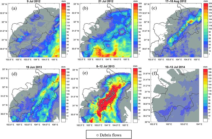
766                                                           Z. Shi et al.: Radar-based quantitative precipitation estimation

main factors, including gravitational potential energy, abun-       to the study of debris flow. Commonly, keeping the eleva-
dant loose materials and meteorological events (Guzzetti et         tion angle close to the ground and estimating the sample cut
al., 2008). The gravitational potential energy remains rela-        at the same height is a basic requirement for radar QPE to
tively stable for a long period of time. The loose materi-          represent the actual rainfall distribution on the ground. The
als are normally made up of sand, unsorted silt, cobbles,           radar beam blocked by the mountain is a serious problem for
gravel, boulders and woody debris (Wang et al., 2016). High-        the low angle observation. The radar beam angle has to be
magnitude earthquake events can generate abundant loose             elevated to avoid the blockage. However, doing this intro-
solid material from co-seismic rock falls and landslides and        duces another problem: rainfall distribution at higher heights
deposited in gullies (Shieh et al., 2009). During the rainy sea-    is different from that at the surface and varies greatly ac-
son, the occurrence of debris flow after an earthquake be-          cording to the precipitation type (Zhang et al., 2012). Er-
comes more frequent (Yu et al., 2014; Guo et al., 2016a).           rors due to radar system calibration and uncertainty in hy-
Both the Ms 8.0 Wenchuan earthquake on 12 May 2008 and              drometeor’s DSD (drop size distribution) also decrease the
the Ms 7.0 Lushan earthquake on 20 April 2013 occurred in           accuracy of rainfall estimates. Therefore, the combination of
the province of Sichuan, China, and have changed the for-           radar and rain gauges to provide accurate rainfall estimates
mation conditions for debris flow. A large number of debris         in complex terrain is attracting increasingly more interest for
flows occurred from 2008 to 2014 and caused many casual-            improving warnings of future precipitation and situational
ties and extensive property damage.                                 awareness (Willie et al., 2017). Furthermore, debris-flow-
   Early warning systems (EWS) for rainfall-induced land-           triggering events are often related to high precipitation gradi-
slide and debris flow are widely implemented in many parts          ents of storms which occur for a short duration and are on a
of the world (Baum and Godt, 2010; Glade and Nadim, 2014;           small scale (Nikolopoulos et al., 2015). Considering this, raw
Segoni et al., 2015). The performance of EWS relies highly          S-band radar reflectivity data are used to estimate rainfall and
on the updating of precipitation thresholds (Rosi et al., 2015).    assess the impact of estimation errors on the identification of
Furthermore, a large amount of loose materials caused by            the I –D threshold over the study area.
earthquake highly increases the occurrence of debris flow              The main aim of this study is to merge the radar QPE,
(Tang et al., 2009, 2012), it is necessary to revaluate the pre-    thereby improving its estimation over complex terrain, and to
cipitation threshold. The model of rainfall intensity–duration      assess the impact of rainfall estimate accuracy on the identi-
(I –D) is widely used to represent the precipitation thresh-        fication of I –D threshold over the study area. To do that,
olds of triggering landslides and debris flow (Aleotti, 2004;       a series of accuracy-improving measures have been adopted
Guzzetti et al., 2007). Some literature concluded that the I –      including a hybrid scan mode, a vertical reflectivity pro-
D relationships for some of the regions were severely af-           file (VPR) correction, a mosaic of reflectivity, a combina-
fected by the Wenchuan earthquake (Su et al., 2012; Cui et          tion of rainfall–reflectivity (R − Z) relationship for convec-
al., 2013; Zhou and Tang, 2014; Guo et al., 2016b). How-            tive and stratiform rainfall, and rainfall bias adjustment with
ever, most of these I –D relationships are derived from rain        Kalman filter (KF). Three radar rainfall estimation scenar-
gauge observation. This is a common technical way to esti-          ios are evaluated with the rain gauge observations for six
mate the I –D thresholds of debris flows using rainfall obser-      debris-flow-triggering rainfall events to validate the accu-
vation from the nearest rain gauge. However, the uncertainty        racy of radar estimate. I –D thresholds are identified from
of I –D thresholds from rain gauge observations could not be        519 rainfall-induced debris flow events with the frequentist
ignored. This is related to two critical limitations which prob-    method (Brunetti et al., 2010; Peruccacci et al., 2012). An-
ably lead to underestimation of observation of strong convec-       other aim of this study is to understand the impact on the
tive events occurring at high-altitude areas. The first limita-     I –D identification due to spatial variability of rainfall ob-
tion is the relatively sparse network density of rain gauges in     servation. Rain gauge observations nearest to the debris flow
the mountainous region (Marra et al., 2014); the other one is       within 10 km and radar observations at the rain gauge loca-
the altitude of gauge deployments, which is at low elevation        tions are used to get the I –D relationship.
for sustainability. The same limitations of rain gauge obser-
vation also exist in the mountainous regions of Sichuan. The
technique of microwave remote sensing has become a nec-             2   Study domain and data
essary way for observing rainfall events in complex terrain.
The radar-based quantitative precipitation estimation (QPE)         The study area is located in Sichuan in southwest China,
has been shown to be useful for the study of debris flows,          which consists of 16 administrative districts and counties.
as its unique advantage of high spatial and temporal resolu-        The area of study is about 38 000 km2 and occupies nearly
tion. Radar observations offer the unique merit of estimating       8 % of the land area of Sichuan (see Fig. 1). This area was
rainfall over the actual debris flow location (David-Novak          strongly affected by the Ms 8.0 Wenchuan earthquake which
et al., 2004; Chiang and Chang, 2009; Marra et al., 2014;           occurred on 12 May 2008 and the Ms 7.0 Lushan earthquake
Berenguer et al., 2015). However, there are many challenges         which occurred on 20 April 2013. In the following years, de-
when radar-based QPE in the mountainous area is applied             bris flow happened frequently. During the period from 2012

Nat. Hazards Earth Syst. Sci., 18, 765–780, 2018                             www.nat-hazards-earth-syst-sci.net/18/765/2018/
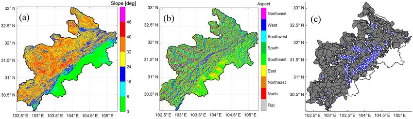
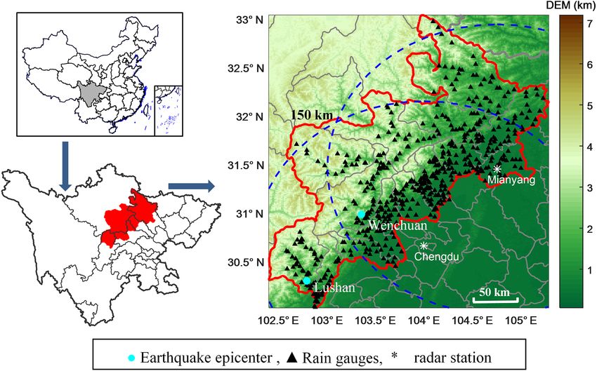
Z. Shi et al.: Radar-based quantitative precipitation estimation                                                                   767

Figure 1. Location and topography of the study area. Asterisks show the location of Chengdu and Mianyang S-band weather radars which
monitor the study area within 150 km (dash black circle) from the radar location. Rain gauges in the study area are marked with black
triangles and mostly deployed in the valley. The two blue circle dots are the epicenter of the Ms 8.0 Wenchuan earthquake on 12 May 2008
and the Ms 7.0 Lushan earthquake on 20 April 2013.

Figure 2. Land use map (a) and lithology map (b) for the study area.

to 2014, the debris flow occurring in this area accounted for          tonic activities, most of the gully is steeply sloped over this
58.3 % of the annual debris flow events which occurred in              area, as shown in Fig. 2b. The main land use types in this
the entire province. The area is in the transitional zone of the       region are mixed forest, cropland and grassland, as shown in
Qinghai–Tibet Plateau to the Sichuan Basin. Terrain changes            Fig. 2a. Potential debris flow watersheds over the study area
steeply and the average altitude above sea level (a.s.l.) for          were extracted from morphological variables, using the lo-
this area is between 500 m and 6 km. The geological struc-             gistic regression method. Berenguer et al. (2015) simplified
ture of the study area shows a northeast to southwest orienta-         the geomorphological variables, as the watersheds maximum
tion. The rocks over this region are mainly comprised of vol-          height (hmax ), mean slope (smean ), mean aspect (θmean ) and
canic rocks, mixed sedimentary rocks, siliciclastic sedimen-           Melton ratio (MR) are the variables with the smallest over-
tary rocks, carbonate sedimentary rocks, acid plutonic rocks,          lapping areas for assessing the susceptibility of the water-
intermediate volcanic rocks, intermediate plutonic rocks, un-          sheds. The hmax , smean , θmean and MR were retrieved from
consolidated sediments, metamorphic rocks, basic plutonic              DEM data. Combined with the debris flow occurrence over
rocks and pyroclastic rocks. Figure 1a shows the litholog-             this area during 3 years, the potential susceptibility map was
ical map. Quaternary deposits were distributed in the form             calculated with the logarithm regression method, as shown
of river terraces and alluvial fans. Owing to frequent tec-

www.nat-hazards-earth-syst-sci.net/18/765/2018/                                 Nat. Hazards Earth Syst. Sci., 18, 765–780, 2018
768 Z. Shi et al.: Radar-based quantitative precipitation estimation
Table 1. Characteristics of S-band Doppler weather radar. severe beam blockage, resulting in inaccurate estimates of
radar rainfall. A number of signal processing techniques have
Items Value been developed to detect and remove clutter and anomalous
Wavelength 10.4 cm
propagation, including fuzzy logic, ground echo maps and
Polarized mode horizontal Gaussian model adaptive processing (GMAP) filters (Harri-
Antenna gain 45 son et al., 2000; Berenguer et al., 2006; Nguyen and Chan-
First side lobe level −29 dBc drasekar, 2013). For the radar data used in this study, ground
Peak transmitted power 750 kW clutter is filtered with the GMAP algorithm configured in the
Noise figure 4 dB Vaisala Sigmet digital processor. Furthermore, in order to
Dynamic range 90 dB overcome the beam blockage and improve the rainfall esti-
Range resolution 300 m mation accuracy, radar data are corrected concerning the fol-
Volume scanning elevation 0.5, 1.5, 2.4, 3.4, 4.3, lowing issues: (i) beam shielding and hybrid scan, (ii) verti-
6.0, 9.5, 14.5, 19.5◦ cal profile of reflectivity, (iii) mosaic of hybrid scan reflectiv-
Altitude above sea level 595 m for Chengdu site
ity, (iv) combination of reflectivity rainfall relationship and
of radar location 557 m for Mianyang site
(v) rainfall bias adjustment.
3.1.1 Beam shielding and hybrid scan
in Fig. 3. The identification results show that there are 673
potential debris flow watersheds in this region. The hybrid scan mode is used to form the initial reflectivity
The climate type of the study area is humid subtropical. field for rainfall estimate by keeping the radar main beam
The monthly precipitation distribution is commonly affected away from the blockage of the complex terrain (Zhang et
by the plateau monsoon, the East Asian monsoon and com- al., 2012). In the study area, the grids with 0.36 km2 reso-
plex terrain. The mean annual rainfall over the central and lution on the ground are aligned with radar bins of each ele-
southern parts of this region varies from 1200 to 1800 mm, vation angle. The blockage coefficients of the low elevation
sometimes even reaching 2500 mm (Xie et al., 2009). The angles at 0.5, 1.5 and 2.4◦ are calculated according to the
mean annual rainfall over the western part of this area is less digital elevation model (DEM), earth curvature, antenna pat-
than 800 mm. The northern and southwestern areas of this tern and the wave propagation model (Pellarin et al., 2002;
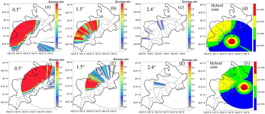
region are in the transition zone from hot dry to humid cli- Krajewski et al., 2006). The blockage ratio distribution of
mates, with mean annual precipitation ranging between 800 two S-band radars can be seen in Fig. 4. There is almost no
and 1200 mm. topographical shielding in the near-field within a distance of
The area is monitored by two well-maintained S-band 50 km from each radar. The main factor considered in the hy-
Doppler weather radars (see Fig. 1). One is deployed in brid scan within 50 km is to meet the estimated rainfall from
Chengdu city at an altitude of 596 m a.s.l. and the other one the same vertical height as much as possible. Thus the area
is deployed at Mianyang city at a height of 557 m a.s.l. Both within 20 km from radar is assigned with elevation angle of
of the radar systems have same system specifications, which 3.4◦ , the area from radar between 20 and 35 km is assigned
can be seen in Table 1. The system provides radar rainfall the elevation angle of 2.4◦ and the area from radar between
estimates at a radial range resolution of 300 m and an angu- 35 and 50 km is assigned the elevation angle of 1.5◦ . It is as-
lar resolution of 1◦ . There is a rain gauge network consisting signed with the elevation angle of 0.5◦ by default when there
of 551 gauges equipped at the meteorological surface station is no blockage over 50 km distance from the radar. The ter-
in the study areas. The number of rain gauges seems to be a rain transforms from plain land to a mountainous region over
lot, but most of them are deployed at the valleys. The den- about 70 km westward of each radar. At this region the alti-
sity of rain gauges is severely scarce at the high altitude of tude rises sharply, and the elevation angle of 0.5◦ is totally
the mountains, resulting in observation gaps where the de- obscured. Therefore, the lowest angle at which the blockage
bris flow initially takes place. The average altitude above sea ratio does not surpass 0.5 is assigned to the aligned grid.
level of those rain gauges is far lower than 3 km. Meanwhile, the blockage ratio is correspondingly used to
compensate the energy loss of reflectivity. The final adaptive-
3 Methods terrain hybrid scan maps are combined as shown in Fig. 4d
and h. It can be seen that most of the study area is covered by
3.1 Radar-accumulated rainfall estimation methods the 1.5 and 2.4◦ radar scans.
S-band weather radar has a unique advantage of being unaf- 3.1.2 Vertical profile of reflectivity
fected by attenuation, as it is subjected to Rayleigh scatter-
ing for almost all hydrometeors. However, in complex terrain Due to the hybrid scan, the radar elevation angle is raised,
conditions, S-band radar observations still face serious chal- resulting in the majority of the observed reflectivity com-
lenges. The main problem comes from ground clutter and ing from the upper levels of precipitation profiles. This is
Nat. Hazards Earth Syst. Sci., 18, 765–780, 2018 www.nat-hazards-earth-syst-sci.net/18/765/2018/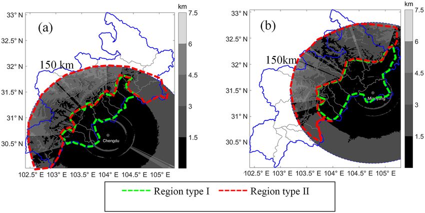
Z. Shi et al.: Radar-based quantitative precipitation estimation                                                                          769

Figure 3. Morphology and potential debris flow watersheds map over study area: (a) slope; (b) aspect; (c) potential debris flow watersheds
(gray polygon) with debris flow observation (blue circle).

Figure 4. Blockage ratio of beam shielding for the radar main lobe beam and hybrid scan map. Panels (a)–(c) represent the blockage ratio of
Chengdu radar at elevations of 0.5, 1.5 and 2.4◦ , respectively. Panels (e)–(g) represent the blockage ratio of Mianyang radar at elevations of
0.5, 1.5 and 2.4◦ , respectively. Hybrid scan maps for Chengdu (d) and Mianyang (h) are merged as long as the blockage ratio is lower than
0.5.

quite different from the actual reflectivity on the ground. It            pacted by the temperature, air dynamics, particle size and
is necessary to account for the reflectivity correction at the            phase are changed along the vertical falling. Figure 5 shows
ground level. This study adopts the VPR method to adjust                  the vertical profile of reflectivity varied approximately as
the reflectivity (Zhang et al., 2012). The processing steps ap-           three piecewise linear sections. Altitude is one the critical
plied in this study are as follows: (i) convection precipitation          factors affecting the atmosphere physics parameters and the
is discriminated from stratiform based on the composite re-               performance of VPR. The areas of study are classified into
flectivity > 50 dBz or VIL > 6.5 kg m−2 , where VIL is verti-             two types, region types I and II, in relation to the height from
cally integrated liquid water content, an estimate of the total           the ground (≤ 1.5 km for region type I and > 1.5 km for re-
mass of precipitation in the clouds (Amburn and Wolf, 1997).              gion type II) and the distance from the radar (≤ 100 km for
(ii) The parameterization of VPR is carried out to generate               region type I and > 100 km for region type II). Figure 6 shows
bright band top, peak, bottom heights and piecewise linear                the identification results for both radars. Apart from the VPR
slopes S1 , S2 and S3 (see Fig. 5). (iii) Observed reflectiv-             adjustment, these two kinds of regions are assessed during
ity is adjusted based on the parameterized VPR to piecewise               the validation of radar QPE in order to understand the actual
extrapolate the corresponding reflectivity at the ground. Fig-            impact of distance and height of radar observations on the
ure 5 shows a sample scatter plot of the vertical reflectivity            rainfall estimation.
profiles from 11:30 to 12:30 UTC+8 on 21 July 2012. Im-

www.nat-hazards-earth-syst-sci.net/18/765/2018/                                     Nat. Hazards Earth Syst. Sci., 18, 765–780, 2018
770                                                              Z. Shi et al.: Radar-based quantitative precipitation estimation

                                                                       ship (Austin, 1987; Rosenfeld et al., 1993) and, theoretically,
                                                                       the R − Z relationships should be adjusted when the DSDs
                                                                       change over the rainfall duration. However, it is still a chal-
                                                                       lenge to obtain fine spatial distribution of DSDs with changes
                                                                       of time over complex terrains. This study adopts the two
                                                                       widely verified R − Z relationships defined as Z = 300R 1.4
                                                                       for convective precipitation (Fulton et al., 1998) and Z =
                                                                       200R 1.6 for stratiform (Marshall et al., 1955), and the rainfall
                                                                       type is identified during VPR processing.

                                                                       3.1.5     Rainfall bias adjustment

                                                                       The errors of the R − Z relationship mainly come from DSD
                                                                       variation, radar calibration errors, etc. (Berne and Krajewski,
                                                                       2013), so the rainfall biases change over time. The mean field
                                                                       bias correction is a method to calculate the ratio of the means
                                                                       of radar estimate and the rain gauge observation (Anagnos-
                                                                       tou and Krajewski, 1999; Chumchean et al., 2003; Yoo and
Figure 5. A real sample of VPR model processed in the study on         Yoon, 2010). In this study, the bias is calculated based on
21 July 2012. The blue circle represents azimuthal mean of reflec-     hourly radar rainfall accumulation and rain gauge accumu-
tivity over 1 h. The orange line represents the idealized VPR with     lated observation. It is defined as
piecewise linear slope α, β and γ . The horizontal blue line is the
                                                                                  1 PN
bright band (BB) top and dashed blue line is BB bottom. The solid                N    i ri
                                                                       BIAS = 1 PN         ,                                       (4)
red line and dashed red line are BB peak and the 0 ◦ C height, re-
                                                                                 N    i gi
spectively.
                                                                       where BIAS is mean rainfall bias in 1 h, g is 1 h accumulated
                                                                       rainfall of rain gauge, i is rain gauge index, r is the radar-
3.1.3   Mosaic of hybrid scan reflectivity
                                                                       based 1 h accumulated rainfall over the ith rain gauge and N
Both S-band radars have common coverage areas where re-                is the total number of rain gauges. As described above, the
flectivity data should be mosaicked to construct a large-scale         density of rain gauge deployment over the mountainous area
sensing for rainfall events. Taking the distance and altitude          is relatively scarce. Therefore the precipitation measured by
as weighing parameters, the mosaic formula is defined as               individual gauges at high and low altitudes may lead to over-
        P                                                              estimation and underestimation, respectively. Therefore, the
            wi × ki × Zi                                               KF is adopted to alleviate the measurements noise of the bias
ZM = iP                  ,                                 (1)
              i wi × ki                                                (Ahnert, 1986; Chumchean et al., 2006; Kim and Yoo, 2014).
                                                                          The basic steps of KF in this study are as follows.
and
          di2
              !                                                          1. State the estimate prediction:
wi = exp − 2 ,                                                 (2)
          L                                                                    BIASP (n) = BIASKF (n − 1) ,                         (5)
              !
          h2i
ki = exp − 2 .                                                 (3)
          H
                                                                               where BIASP represents the bias prediction, BIASKF
Here, ZM represents the mosaicked hybrid scan reflectivity,                    represents the bias estimate update and n is discrete
Zi is the single radar hybrid scan reflectivity, i is the radar                time.
index, w is weighing component for the horizontal weighting
                                                                         2. State the estimate error covariance prediction:
and k is weighing component for the vertical weighting. The
variable d is the distance between the analysis grid and the                   PP (n) = F 2 × PKF (n − 1) + Q,                      (6)
radar, and h is the height above the ground of the single radar
hybrid scan. The parameters L and H are scale factors of the
two weighting functions.
                                                                               where PP represents the bias estimate error covariance
3.1.4   Combination of rainfall relationship                                   prediction, PKF represents the bias estimate error co-
                                                                               variance update and Q represents covariance function
Rainfall rates are calculated from radar reflectivity by a                     of the system error.
power law empirical relationship called the R − Z relation-

Nat. Hazards Earth Syst. Sci., 18, 765–780, 2018                                  www.nat-hazards-earth-syst-sci.net/18/765/2018/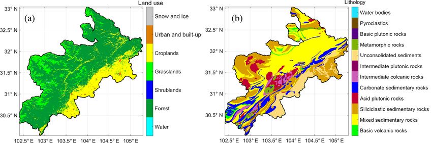
Z. Shi et al.: Radar-based quantitative precipitation estimation                                                                         771

Figure 6. The height from the ground of hybrid scan for two S-band radar (a) radar located at Chengdu (b) radar located at Mianyang. The
regions surrounded by green dash lines meet the condition of that the height from the ground is 1.5 km below and the distance from radar is
inner 100 km and is recognized as region type I. The regions surrounded by the red dash lines represents the area under the opposite condition
and is recognized as region type II.

  3. Calculate the Kalman gain:                                          Calculating the event duration (D) and the average inten-
                                                                         sity (I ) requires the start and end times of the rainfall event.
      G (n) = PP (n) × (PP (n) + S)−1 ,                            (7)   The duration and intensity of each debris flow can be di-
                                                                         rectly identified with the time-sequential radar rainfall esti-
                                                                         mate. These times are determined by an interval of at least
      where G represents the Kalman gain. S represents co-               24 h, rain rates of less than 0.1 mm h−1 (Guzzetti et al., 2008;
      variance function of the measurement error.                        Marra et al., 2014) or corresponding radar reflectivity of less
                                                                         than 10 dBz to separate two consecutive rainfall events. The
  4. Update the state estimate:                                          parameters of a and β are estimated with the frequentist
                                                                         method (Brunetti et al., 2010).
      BIASKF (n) = BIASP (n) + G (n) × [BIASm (n) − BIASP (n)],    (8)      In order to illustrate the impacts of radar rainfall estimate
                                                                         on I –D threshold, basic procedures of the frequentist method
                                                                         are applied to radar rainfall accumulation and are described
      where BIASm represents the bias measurement.                       below:

  5. Update the estimate error covariance:                                  i. Radar-identified rainfall durations and average intensi-
                                                                               ties are log transformed as log(I ) and log(D). Both of
      PKF (n) = (1 − G (n)) × PP (n) .                             (9)         them are fitted by least-squares method to form a lin-
                                                                               ear equation as log(If ) = log(α50 )−βlog(D), where α50
                                                                               and β are the fitted intercept and slope, respectively.

  It is assumed that the variation of the real bias within each            ii. For each debris flow, the difference δ(D) between the
hour is negligible, and the initial estimator for mean field                   actual rainfall average intensity log[I (D)] and the cor-
radar rainfall logarithmic bias and its error variance are as-                 responding fitted intensity value log[If (D)] is calcu-
sumed to equal their updated values, which are, respectively,                  lated: δ(D) = log[I (D)] − log[If (D)].
BIASKF (0) and PKF (0).                                                   iii. The probability density function (PDF) of the δ(D) dis-
                                                                               tribution is determined through kernel density estima-
3.2   Intensity–duration threshold identification
                                                                               tion and furthermore fitted with a Gaussian function,
      methods
                                                                               which is defined as
                                                                                                            !
Rainfall thresholds for the possible initiation of debris flows                                    (δ − b)2
are identified according to the I –D power law relationship                    f (δ) = a × exp −              ,                   (11)
                                                                                                      2c2
(Guzzetti et al., 2007), it is defined as follows:

I = αD −β .                                                       (10)         where a > 0, c > 0 and a, b and c ∈ R.

www.nat-hazards-earth-syst-sci.net/18/765/2018/                                     Nat. Hazards Earth Syst. Sci., 18, 765–780, 2018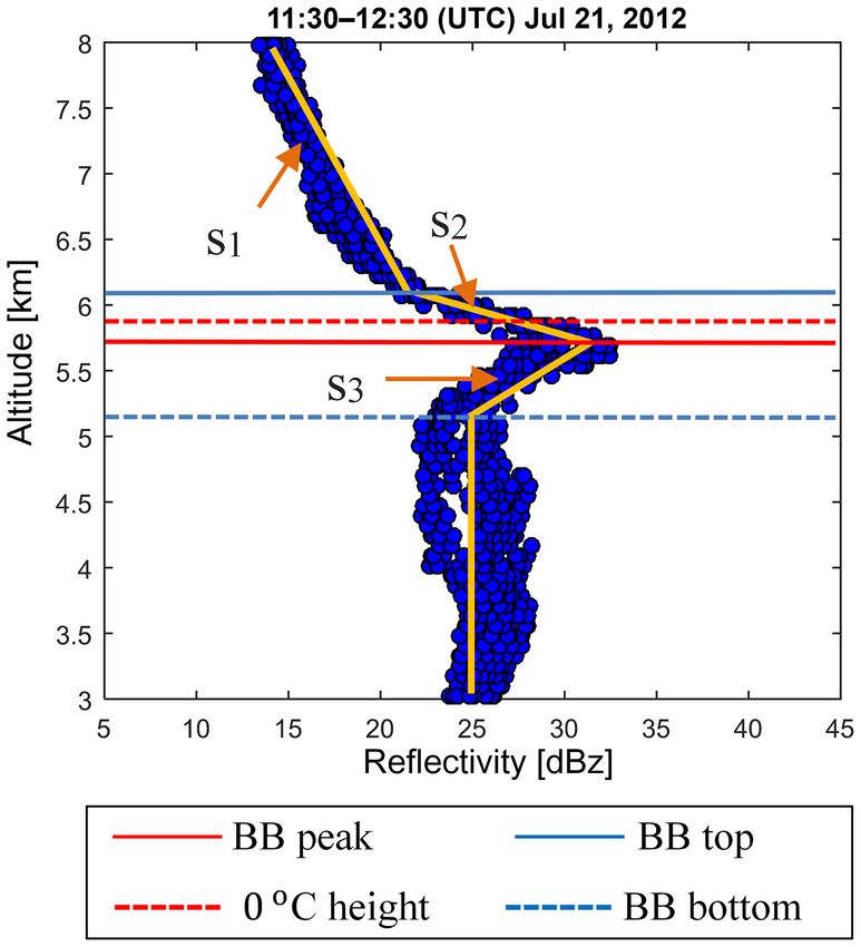
772                                                          Z. Shi et al.: Radar-based quantitative precipitation estimation

    iv. The threshold for expected minimum exceedance prob-        of rainfall observation and positioning, a series of process-
        ability (Pmep ) is determined by PDF function, as          ing steps including hybrid scan, VPR correction, a combined
        Z δmep                                                     R − Z relationship and mean bias adjustment are performed
               f (δ)dδ = Pmep ,                           (12)     on six rainfall events to improve the accuracy of radar-based
        −∞                                                         accumulated rainfall. In order to evaluate the overall perfor-
                                                                   mance and verify the impact on I –D threshold due to rain-
       where δmep is the intercept parameters. δmep can be re-     fall accumulation accuracy, the assessment was performed
       solved through Eq. (12) for given Pmep and then the         on three scenarios of radar-based estimates: scenario I, the
       αmep corresponding to the Pmep is calculated as             estimate from raw data of hybrid scan without VPR and bias
                                                                  adjustment; scenario II, the estimates with VPR adjustment
       αmep = α50 exp δmep .                             (13)      after scenario I; and scenario III, the estimates with rainfall
                                                                   bias correction after scenario II. According to rainfall esti-
                                                                   mate evaluation, I –D thresholds are derived from those sce-
       Finally, αmop and β are the best-fitted parameters for      narios and also assessed with regard to accuracy and spatial
       exceedance probabilities Pmep .                             resolution.
   The minimum exceedance probability is set to 5 % for this       4.1   Assessment of rainfall estimation accuracy
study.
                                                                   The accuracy of the radar-based rainfall event accumula-
                                                                   tion is assessed with the rain gauge observations. In order to
4     Events, results and discussion
                                                                   perform an evaluation, a set of criteria is calculated includ-
Six debris-flow-triggering rainfall events which occurred in       ing normalized standard error (NSE), normalized mean bias
the area of study between 2012 and 2014 are analyzed. Those        (NMB) and correlation coefficient (CORR), defined as
events happened at the most severely earthquake-affected re-                 1 PN
                                                                            N    i |ri − gi |
gion during rainy season and triggered a total of 519 debris       NSE =        1 PN
                                                                                              × 100 %,                       (14)
flows that caused casualties and extensive property damage.                     N    i gi
                                                                              1 PN
Table 2 summarizes the characteristics of the rainfall events.                      (ri − gi )
Three events occurred in August, two events occurred in July       NMB = N 1i PN               × 100 %,                      (15)
                                                                                 N     i gi
and one occurred in June. These events are deemed to be                             PN
representative of the debris-flow-triggering precipitation in                             (gi − g) (ri − r)
                                                                   CORR = qP i                  q                 ,          (16)
the region during the rainy season. The event duration and                         N           2 PN             2
                                                                                   i (gi − g)         i (ri − r)
maximum rainfall accumulation are also retrieved by the rain
gauge nearest to debris flow location and radar observations.      where NMB and NSE are in percent, CORR is dimension-
The identification of the rainfall event was determined by an      less, ri and gi represent the rainfall accumulation from radar
interval of at least 24 h, during which the rain rate is less      and gauge and N is the total sampling number. The statistical
than 0.1 mm h−1 (Guzzetti et al., 2008; Marra et al., 2014).       criteria comparisons between rain gauges and the three radar
Table 2 indicates that the durations and rainfall accumula-        estimate scenarios are shown in Table 3, and the scatter plot
tions identified by gauge and radar are different due to the       of radar-based estimates and rain gauge rainfall observations
precipitation type and density of rain gauges. The identifi-       is shown in Fig. 8. The comparison of scenario I indicates
cation differences of event nos. 1, 2 and 6 between gauge          that the NSE, NMB and CORR of the study areas are 50.7,
and radar are not as large as event nos. 3, 4 and 5. From          −41.1 % and 0.78, respectively. The radar-based rainfall is
Fig. 7, showing radar-estimated rainfall accumulation for the      underestimated. The linear ratio is estimated from linear re-
six rainfall events (the improving measures described below        gression of radar rainfall estimation and rain gauge obser-
are applied in Fig. 7), it can be seen that the precipitation      vation, with the predefined intercept of zero. The linear ra-
of event nos. 3, 4 and 5 is dominated by convection and the        tio approximates to 1 when radar-based rainfall estimation
strong core of rainfall regions is located in the high-altitude    is consistent with rain gauge observation. The linear ratio of
area where rain gauges are relatively scarce. A few debris         rainfall observation between radar and gauge for scenario I is
flow events occurred in the long range, approaching radar          0.51, as shown in Fig. 8a. The reason for the underestimation
detection edges, while the rainfall measured there was low.        is the systematic bias and uncertainty of reflectivity on the
This may be caused by the decreasing resolution at long ra-        ground. From the comparison of two types of regions, it can
dial range. In following section, rainfall estimation accuracy,    be observed that the NSE, NMB and CORR of region type I
I –D, the distance and height are considered as evaluation         are relatively better than region type II. It is revealed that im-
factors to assess the radar-based rainfall estimate.               proved measures are needed for the hybrid scan estimate.
   Considering the accuracy and robustness of the I –D                The comparison of scenario II indicates that the NSE,
threshold of the debris flow are determined by the accuracy        NMB and CORR for the study areas are 46.1, −18.6 % and

Nat. Hazards Earth Syst. Sci., 18, 765–780, 2018                            www.nat-hazards-earth-syst-sci.net/18/765/2018/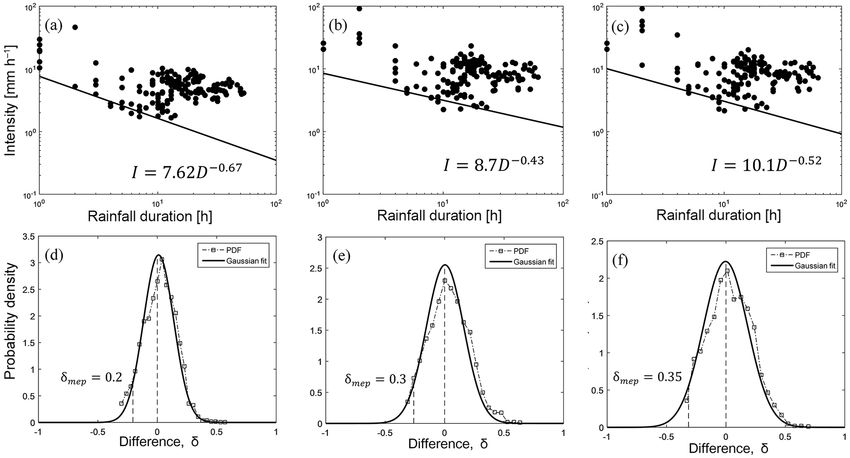
Z. Shi et al.: Radar-based quantitative precipitation estimation                                                                          773

Figure 7. Images of radar-estimated rainfall accumulation for the six rainfall events (a–f). Circles represent the location of triggered debris
flows. Events are shown in chronological order: (a) 9 July 2012; (b) 21 July 2012; (c) 17–18 August 2012; (d) 19 June 2013; (e) 8–
12 July 2013; (f) 10, 12 July 2014.

Table 2. Characteristics of the rainfall events.

           Event     Date                  Number of     Event duration    Event duration         Max. rainfall      Max. rainfall
           no.                               triggered          by rain          by radar     accumulation by     accumulation by
                                          debris flows       gauge (h)                (h)     rain gauge (mm)         radar (mm)
           1         9 Jul 2012                      9               12                 11                17.5                29.6
           2         21 Jul 2012                     9               10                 12                29.3                23.6
           3         17–18 Aug 2012                200                7                 49                19.2               195.8
           4         19 Jun 2013                    15                5                 12                55.3               101.8
           5         8–12 Jul 2013                 261               55                 73               562.2               416.9
           6         10–12 Jul 2014                 25               20                 21                28.5                17.8

0.80, respectively. This is an improvement over scenario I.               and 0.84, respectively. The linear ratio of rainfall observa-
The radar-based rainfall is also underestimated through the               tion between radar and gauge is 0.98, as shown in Fig. 8c,
VPR adjustment, and the linear ratio of rainfall observation              and this means the consistency between rainfall and radar ob-
between radar and gauge is 0.76, as shown in Fig. 8b. This                servation is achieved through the KF-based bias correction.
means rainfall biases still exist in the estimate. The NSE and            Figure 9 shows the average and covariance of bias estimation
CORR of region type I are also slightly better than region                by KF and mean field bias method for six rainfall events. The
type II.                                                                  CORR and NSE improvement also verifies the efficiency of
   The comparison of scenario III indicates that the NSE,                 the KF for radar QPE in mountainous areas. Kalman filter-
NMB and CORR of the entire study area are 44.0, 1.91 %

www.nat-hazards-earth-syst-sci.net/18/765/2018/                                     Nat. Hazards Earth Syst. Sci., 18, 765–780, 2018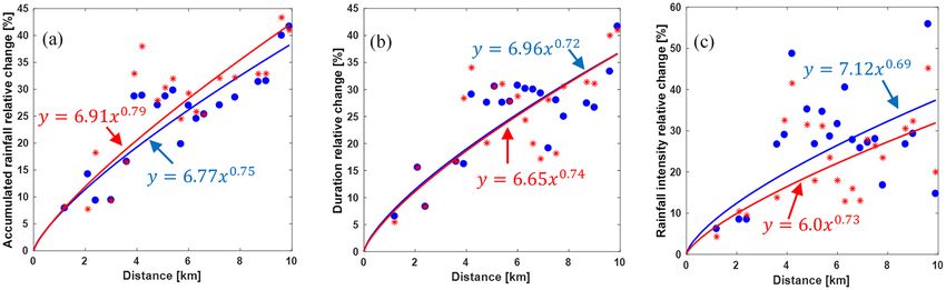
774                                                               Z. Shi et al.: Radar-based quantitative precipitation estimation

Figure 8. Scatter plots of radar and rain gauge event–rainfall accumulations. (a) Scenario 1: radar estimate from hybrid scan. (b) Scenario 2:
radar estimate from hybrid scan and VPR. (c) Scenario 3: radar estimate through the hybrid scan, VPR and bias correction.

Table 3. The comparison of radar and rain gauge for each estimate scenario.

           Criteria         Scenario I (hybrid scan)                Scenario II (VPR)               Scenario III (bias adjustment)
                        Region     Region     All study       Region     Region    All study       Region     Region     All study
                         type I    type II     regions         type I    type II    regions         type I    type II     regions
           NSE (%)        46.4         50         50.7          45.8      49.0         46.1           43.5       47.2         44.0
           NMB (%)       −40.9      −42.8        −41.1         −17.1     −21.2        −18.6            1.7       10.8         1.91
           CORR           0.80       0.77         0.78          0.82      0.77         0.80           0.85       0.82         0.84

                                                                         Table 4. The parameters of Gaussian fitting, which are used by the
                                                                         frequentist method to account for I –D threshold.

                                                                              Parameters of      Scenario I    Scenario II   Scenario III
                                                                              Gaussian fitting
                                                                              a                      3.144           2.55           2.22
                                                                              b                      0.011          0.003         −0.003
                                                                              c                     0.1273         0.1578         0.1868

                                                                         scenarios is shown in Fig. 10. Comparisons of scatter distri-
                                                                         bution between scenarios I, II and III indicate that the average
Figure 9. The average and covariance of bias estimation by Kalman        rainfall intensity and duration are incrementally increased
filter and mean field bias method for six rainfall events.               when applying the improvement measures. The PDF estima-
                                                                         tions reveal that the number of positive differences δ(D) is
                                                                         more than the number of negative differences. This can be
ing frees the entire rainfall event estimate of large significant        accounted for by storm triggering, which is relatively dom-
overestimation or underestimation.                                       inant. The parameters of the Gaussian function are summa-
   Scenario III provides the optimum rainfall estimation for             rized in Table 4. Parameter a incrementally decreases. When
this study. In the following, all three scenarios are used to as-        applying the improvement measures, parameter c has the op-
sess the impact of QPE accuracy on I –D relationship identi-             posite trend and parameter b randomly changes in a small
fication.                                                                range around zero.
                                                                            The I –D threshold derived from the scenario III is
4.2   Intensity–duration thresholds based on radar QPE
                                                                         10.1D −0.52 . It is higher than the other two I –D thresholds
The radar rainfall estimates with high spatial resolution                derived from scenario I and scenario II, due to application of
can retrieve rainfall duration and average intensity for each            accuracy improving measuring.
rainfall-triggered debris flow, so an abundant of sample data
are captured to induce the I –D relationship. Scatter distribu-
tion of event duration–intensity for the three radar-estimated

Nat. Hazards Earth Syst. Sci., 18, 765–780, 2018                                   www.nat-hazards-earth-syst-sci.net/18/765/2018/
Z. Shi et al.: Radar-based quantitative precipitation estimation 775
Figure 10. Scatter plots of radar and rain gauge event–rainfall accumulation and probability density functions (PDFs). Panels (a), (b)
and (c) are the scatter plots of scenario I, II and III, respectively. Panels (d), (e) and (f) are the Gaussian fitted PDF of scenario I, II and III,
respectively.
quired to be more than 1 h and minimum mean rainfall rate
is 0.1 mm h−1 . (2) The maximum distance from debris flow
location is less than 10 km. (3) The identification of I –D
threshold is calculated from frequentist methods with ex-
ceedance probabilities of 0.5 %. Firstly, the event’s rainfall
accumulation is compared between rain gauge observations
nearest to the location of debris flows and radar estimates at
the location of the corresponding rain gauge. The scatter plot
of rain gauge and radar estimates is shown in Fig. 11. The
corresponding metrics are calculated. The CORR is 0.88,
NMB is 17.07 %, NSE is 28.32 % and the linear ratio is
1.13, indicating that rainfall observations from the rain gauge
nearest to the debris flow location and radar estimates at co-
Figure 11. Event–rainfall scatter plots of rain gauges nearest to de- location have the tendency of consistency. The I –D thresh-
bris flow locations and radar-based estimate from scenario III over olds are derived from rain gauge and radar estimates. Scatter
the same location of rain gauge. plots of I –D pairs are shown in Fig. 12. The I –D threshold
estimated from rain gauges is I = 5.1D −0.42 . The other I –D
threshold estimated from radar is I = 5.8D −0.41 . Both I –D
4.3 Comparison with intensity–duration thresholds thresholds seem slightly lower than I = 10.1D −0.52 , since
from rain gauge observations the scarce gauge network did not capture the strong core of
rainfall which triggered the debris flow. It is interesting to
In order to analyze the impact of the spatial sampling vari- note that I –D thresholds of both radar and rain gauge are
ability on identification of I –D threshold for radar estimates very similar, although there are some measurement errors be-
and rain gauge observations, I –D thresholds are derived tween them, as shown in Fig. 11.
from the rain gauge nearest to the debris flow and radar es-
timates at the corresponding co-location of the rain gauge
(Marra et al., 2014). There are some same predefined condi-
tions for comparison: (1) duration times are identified sepa-
rately by two kinds of sensors, rainfall duration time is re-
www.nat-hazards-earth-syst-sci.net/18/765/2018/ Nat. Hazards Earth Syst. Sci., 18, 765–780, 2018776 Z. Shi et al.: Radar-based quantitative precipitation estimation
Figure 12. Intensity–duration thresholds (black line) derived from (a) rain gauges nearest to debris flow locations and (b) radar rainfall
estimation at the same location of the rain gauges nearest to the debris flow.
Figure 13. Scatter plot of relative changes versus distance. Blue circles represent relative change between radar estimate at debris flow
location and rain gauge observation nearest to debris flow location. Red asterisks represent relative change between radar estimate at debris
flow location and radar estimate at the co-location of the nearest rain gauge. (a) Accumulated rainfall relative change. (b) Duration relative
change. (c) Rainfall intensity relative change.
4.4 Impact of rainfall spatial variation on intensity and referred value. (3) The maximum distance from debris flow
duration location to the nearest rain gauge is predefined within 10 km
and the distance resolution is set equal to the range resolu-
tion of 300 m of the China New Generation Doppler Weather
The accumulated rainfall, duration and rainfall intensity Radar (CINRAD). (4) In order to assess the rainfall spatial
identified from the nearest rain gauge probably are differ- variation using a multi-sensor, the radar-based estimate at the
ent from the realities occurred at the debris flow location, co-location of the nearest rain gauge, as well as rain gauge
since the rainfall varies in space especially for convective observations, is also compared with the radar-based estimate
precipitation with sharp variation in short distance. The ob- at the location of debris flow.
served rainfall differences rely on the distance from the near- The metrics of accumulated rainfall relative change
est rain gauge to the debris location and could be considered (ARRC), duration relative change (DRC) and rainfall inten-
as rainfall spatial change. To this end, relative changes of sity relative change (RIRC) are calculated for the nearest rain
the accumulated rainfall, duration and rainfall intensity ver- gauge and radar estimate at the co-location. The results of
sus distance are calculated from the comparisons with the ARRC, DRC and RIRC versus distance are shown in Fig. 13.
radar-based estimate at the location of debris flow. The met- The main findings from the evaluation results are summa-
rics for evaluating relative change versus distance are defined rized as follows:
in Table 5. There are also some predefined conditions for
the comparison of relative changes versus distance. (1) The 1. The results of ARRC, DRC and RIRC all have an en-
radar rainfall estimations used for comparison are all from larging tendency along with the increasing distance. The
scenario III. (2) The radar rainfall estimations and duration maximum ARRC, DRC and RIRC for rain gauge obser-
identification at the debris flow location are considered as the vations are 42.2, 41.67 and 55.88 %, respectively. The
Nat. Hazards Earth Syst. Sci., 18, 765–780, 2018 www.nat-hazards-earth-syst-sci.net/18/765/2018/Z. Shi et al.: Radar-based quantitative precipitation estimation 777
Table 5. The metric for assessing the relative changes of the accumulated rainfall, duration and rainfall intensity versus distance.
Factors Rain gauge observation nearest to debris flow Radar estimate at the co-location of rain gauge
location versus radar estimate at debris flow lo- versus radar estimate at debris flow location
cation
PN(s) PN(s)
i=1 |Rdf (i)−Rg (i)| i=1 |Rdf (i)−Rr (i)|
Accumulated rainfall relative ARRCg (s) = PN(s) × 100 % ARRCr (s) = PN(s) × 100 %
change (ARRC) i=1 Rdf (i) i=1 Rdf (i)
PN(s) PN(s)
i=1|Ddf (i)−Dg (i)| i=1|Ddf (i)−Dr (i)|
Duration relative change DRCg (s) = PN(s) × 100 % DRCr (s) = PN(s) × 100 %
(DRC) i=1 Ddf (i) i=1 Ddf (i)
PN(s) PN(s)
i=1|Idf (i)−Ig (i)| i=1|Idf (i)−Ir (i)|
Rainfall intensity relative RIRCg (s) = PN(s) × 100 % RIRCr (s) = PN(s) × 100 %
change (RIRC) i=1 Idf (i) i=1 Idf (i)
Note: R represents accumulated rainfall for debris flow event, D represents duration for rainfall event and I represents the mean intensity for rainfall event. The variables with
subscript df, g and r represent the observation from radar at debris flow location, rain gauge nearest to debris flow location and radar at the co-location of the nearest rain gauge,
respectively. s represents the distance between the nearest rain gauge location and debris flow location with the range resolution of 300 m. N(s) represent the number of rain gauge
observation for debris flow at the distance of s .
Table 6. Parameters of the identified ID thresholds and relative changes.
α−αS3 β−βS3
α αS3 × 100 % β βS3 × 100 %
Scenario I 7.62 −24.5 0.67 28.8
Scenario II 8.7 −13.8 0.43 −17.3
Scenario III 10.1 0.0 0.52 0.0
Rain gauges 5.1 −49.5 0.42 −19.2
Radar estimate at the co-location
of the nearest rain gauge 5.8 −42.6 0.41 −21.2
Note: αS3 and βS3 are α and β , respectively, estimated from scenario III.
maximum ARRC, DRC and RIRC for radar-based es- Concerning rainfall spatial variation, the relative change of α
timate at the co-location of the nearest rain gauge are for the nearest gauge observation and radar-based estimate at
43.33, 41 and 45.2 %, respectively. the co-location is −49.5 and −42.6 %, respectively. The rela-
tive change of β for the nearest gauge observation and radar-
2. Nonlinear regression is applied for ARRC, DRC and based estimate at the co-location is −19.5 and −21.2 %, re-
RIRC versus distance to investigate the average ten- spectively. The relative change of α is remarkably larger than
dency, as shown in Fig. 13. The regression curves of the one derived from radar-based estimate on the debris flow
ARRC and DRC for rain gauge and radar are simi- location, but the differences of α and β for rain gauges and
lar, within 10 and 4 km, respectively, indicating the ob- radar-based estimate at the co-location are not significant.
served difference as a function of distance is dominated
by the natural spatial variability and the potential im- 4.5 Comparison with previous results
pact from differences in rainfall estimates coming from
different sensors is secondary, especially for estimating The I –D threshold for the study regions is compared with
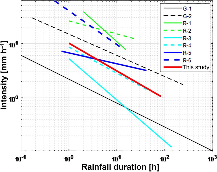
duration. other global and regional thresholds in the literature. It can
be seen from Fig. 14 that the threshold obtained in this work
It is clear from the above discussion that the rainfall esti- (red in Fig. 14) falls in the range of other I –D thresholds.
mation accuracy and spatial variation impact the identifica- The results were also compared with the rainfall thresholds
tion of I –D threshold. We further take the α and β estimated previously proposed in the Wenchuan earthquake area (Tang
from scenario III as a reference value and calculate the rel- et al., 2012; Zhou and Tang, 2014; Guo et al., 2016a). Our
ative change of α and β for each scenario, as shown in Ta- result lies in the middle range of them. The difference comes
ble 6. The relative change of α for scenarios I, II and III is from the database we used, the radar data which are used
−24.5, −13.8 and 0 %, respectively. The relative change of to fill the observation gap of rain gauges, and the identifica-
β for scenarios I, II and III is −28.8, −17.3 and 0 %, respec- tion method of I –D threshold that was also different due to a
tively. It is indicated that improving the accuracy of rainfall different exceedance probability. The I –D threshold of this
estimate is able to decrease the relative changes of α and β. study was cross-checked with that proposed in the area af-
www.nat-hazards-earth-syst-sci.net/18/765/2018/ Nat. Hazards Earth Syst. Sci., 18, 765–780, 2018778 Z. Shi et al.: Radar-based quantitative precipitation estimation
estimation from radar are performed and compared with
rain gauge observations to validate the accuracy. The re-
sults show that the combination of all correction proce-
dures reduces the bias to 1.91 % and the NSE to 44 %
and improves the correlation coefficient to 0.84 and the
linear ratio to 0.98.
b. Intensity–duration rainfall thresholds for the trigger-
ing debris flow are calculated with a frequentist ap-
proach. The I –D threshold of I = 10.1D −0.52 is de-
rived from the KF-corrected radar estimates. The accu-
mulated rainfall is lower than rain gauge observations
and the derived I –D is also underestimated. The hybrid
scan, VPR correction and combination of R − Z rela-
tionship are strongly required.
Figure 14. I –D thresholds determined for this study (red line)
c. The I –D deduced from rain gauge observations nearest
and those of various other studies. G is global and R is region.
to the occurrence of debris flow is highly similar to the
G-1: Guzzetti et al. (2008); G-2: Caine (1980); R-1: Wenchuan
earthquake area (Zhou and Tang, 2014); R-2: Qingping, a re- one deduced from the radar estimates at the same loca-
gion in Wenchuan earthquake area (Tang et al., g120 2012); R-3: tion as rain gauge: I = 5.1D −0.42 and I = 5.8D −0.41 ,
Wenchuan earthquake area (Guo et al., 2016a); R-4: Italy (Marra et respectively. These I –D thresholds are underestimated
al., 2014); R-5: central Taiwan (Jan and Chen, 2005); R-6: Japan due to the rainfall spatial variation and the noncontinu-
(Jibson, 1989). ous sampling effect.
Finally, it is clear that radar-based rainfall estimates and
fected by the Chi-Chi earthquake in Taiwan (Chien Yuan et thresholds supplement the monitoring gaps of EWS where
al., 2005), mainly due to the climatic differences like storm rain gauges are scarce. A better understanding of the re-
occurrence duration and intensity. The result nearly over- lationship between rainfall and debris flow initiation for
lapped with the one proposed in Adige, Italy (Marra et al., earthquake-affected areas can be gained by improving the
2014). Guzzetti et al. (2008) updated the global I –D thresh- spatiotemporal resolution and low-elevation-angle coverage
old, which is significantly lower than the global threshold of radar observation, especially for monitoring the convec-
first proposed by Caine (1980). Our result is higher than that tive storm occurring at the mountains.
for the world (Guzzetti et al., 2008).
Data availability. The data used in this research can be made avail-
5 Summary able on demand. Please contact the authors for requests.
The main purpose of this paper is to evaluate the debris flow
occurrence thresholds of the rainfall intensity–duration in Competing interests. The authors declare that they have no conflict
the earthquake-affected areas of Sichuan over the rainy sea- of interest.
sons from 2012 to 2014. The paper calculates the intensity–
duration threshold from radar-based rainfall estimates, which
is different from the common method of using rain gauge ob- Special issue statement. This article is part of the special issue
servation. Radar observations have high spatial resolutions “Landslide early warning systems: monitoring systems, rainfall
thresholds, warning models, performance evaluation and risk per-
sensitive to convective precipitation, which is a critical issue
ception”. It is not associated with a conference.
for rain gauge observation due to its scarcity and low-altitude
deployment over mountainous areas. However, the accuracy
of radar-based QPE over complex areas is affected by the Acknowledgements. This research was supported by the National
terrain and remains a challenge for hydrological application. Natural Science Foundation of China (no. 41505031), the Science
The following work was done to draw the conclusions. and Technology Support Project of Sichuan (no. 2015SZ0214),
China Meteorological Bureau Meteorological Sounding Engineer-
a. Two S-band Doppler radars covered the study area.
ing Technology Research Center funding, China Scholarship Coun-
Radar observations for six rainfall events were pro- cil (no. 201508515021), and scientific research funding of CUIT
cessed with a series of mountain-oriented QPE algo- (no. J201603). We thank the weather bureau of Sichuan for the data
rithms, including a terrain-adapted hybrid scan, VPR services.
correction, a reflectivity mosaic, a combination of R−Z The participation of VC is supported by the US National Science
relationships a rainfall bias correction. Three types of Foundation through the Hazard SEES program.
Nat. Hazards Earth Syst. Sci., 18, 765–780, 2018 www.nat-hazards-earth-syst-sci.net/18/765/2018/Z. Shi et al.: Radar-based quantitative precipitation estimation 779
Fulton, R. A., Breidenbach, J. P., Seo, D.-J., Miller, D. A., and
Edited by: Samuele Segoni O’Bannon, T.: The WSR-88D rainfall algorithm, Weather Fore-
Reviewed by: three anonymous referees cast., 13, 377–395, 1998.
Glade, T. and Nadim, F.: Early warning systems for nat-
ural hazards and risks, Natural Hazards, 70, 1669–1671,
https://doi.org/10.1007/s11069-013-1000-8, 2014
References Guo, X., Cui, P., Li, Y., Ma, L., Ge, Y., and Mahoney, W. B.:
Intensity–duration threshold of rainfall-triggered debris flows in
Ahnert, P.: Kalman filter estimation of radar-rainfall field bias, the Wenchuan earthquake affected area, China, Geomorphology,
Preprints of the 23rd Conference on Radar Meteorology, 1986. 253, 208–216, 2016a.
Aleotti, P.: A warning system for rainfall-induced Guo, X., Cui, P., Li, Y., Zou, Q., and Kong, Y.: The formation and
shallow failures, Eng. Geol., 73, 247–265, development of debris flows in large watersheds after the 2008
https://doi.org/10.1016/j.enggeo.2004.01.007, 2004. Wenchuan Earthquake, Landslides, 13, 25–37, 2016b.
Amburn, S. A. and Wolf, P. L.: VIL density as a hail indicator, Guzzetti, F., Peruccacci, S., Rossi, M., and Stark, C. P.: Rainfall
Weather Forecast., 12, 473–478, 1997. thresholds for the initiation of landslides in central and southern
Anagnostou, E. N. and Krajewski, W. F.: Real-time radar rainfall es- Europe, Meteorol. Atmos. Phys., 98, 239–267, 2007.
timation. Part I: Algorithm formulation, J. Atmos. Ocean. Tech., Guzzetti, F., Peruccacci, S., Rossi, M., and Stark, C. P.: The rainfall
16, 189–197, 1999. intensity–duration control of shallow landslides and debris flows:
Austin, P. M.: Relation between measured radar reflectivity and sur- an update, Landslides, 5, 3–17, 2008.
face rainfall, Mon. Weather Rev., 115, 1053–1070, 1987. Harrison, D., Driscoll, S., and Kitchen, M.: Improving precipitation
Baum, R. L. and Godt, J. W.: Early warning of rainfall-induced shal- estimates from weather radar using quality control and correction
low landslides and debris flows in the USA, Landslides, 7, 259– techniques, Meteorol. Appl., 7, 135–144, 2000.
272, 2010. Jan, C. D. and Chen, C. L.: Debris flows caused by Typhoon Herb in
Berenguer, M., Sempere-Torres, D., Corral, C., and Sánchez- Taiwan, in: Debris Flow Hazards and Related Phenomena, edited
Diezma, R.: A fuzzy logic technique for identifying nonprecipi- by: Jakob, M. and Hungr, O., Springer, Berlin Heidelberg, 363–
tating echoes in radar scans, J. Atmos. Ocean. Tech., 23, 1157– 385, 2015.
1180, 2006. Jibson, R. W.: Debris flows in southern Puerto Rico, Geol. S. Am.
Berenguer, M., Sempere-Torres, D., and Hürlimann, M.: Debris- S., 236, 29–56, 1989.
flow forecasting at regional scale by combining susceptibility Kim, J. and Yoo, C.: Use of a dual Kalman filter for real-time correc-
mapping and radar rainfall, Nat. Hazards Earth Syst. Sci., 15, tion of mean field bias of radar rain rate, J. Hydrol., 519, 2785–
587–602, https://doi.org/10.5194/nhess-15-587-2015, 2015. 2796, https://doi.org/10.1016/j.jhydrol.2014.09.072, 2014.
Berne, A. and Krajewski, W. F.: Radar for hydrology: Unful- Krajewski, W. F., Ntelekos, A. A., and Goska, R.: A GIS-based
filled promise or unrecognized potential?, Adv. Water Resour., methodology for the assessment of weather radar beam blockage
51, 357–366, https://doi.org/10.1016/j.advwatres.2012.05.005, in mountainous regions: two examples from the US NEXRAD
2013. network, Comput. Geosci., 32, 283–302, 2006.
Brunetti, M. T., Peruccacci, S., Rossi, M., Luciani, S., Valigi, D., Marra, F., Nikolopoulos, E. I., Creutin, J. D., and Borga, M.: Radar
and Guzzetti, F.: Rainfall thresholds for the possible occurrence rainfall estimation for the identification of debris-flow occur-
of landslides in Italy, Nat. Hazards Earth Syst. Sci., 10, 447–458, rence thresholds, J. Hydrol., 519, 1607–1619, 2014.
https://doi.org/10.5194/nhess-10-447-2010, 2010. Marshall, J., Hitschfeld, W., and Gunn, K.: Advances in radar
Caine, N.: The rainfall intensity: duration control of shallow land- weather, Adv. Geophys., 2, 1–56, 1955.
slides and debris flows, Geogr. Ann. A, 62, 23–27, 1980. Nguyen, C. M. and Chandrasekar, V.: Gaussian Model
Chiang, S.-H. and Chang, K.-T.: Application of radar data to model- Adaptive Processing in Time Domain (GMAP-TD) for
ing rainfall-induced landslides, Geomorphology, 103, 299–309, Weather Radars, J. Atmos. Ocean. Tech., 30, 2571–2584,
https://doi.org/10.1016/j.geomorph.2008.06.012, 2009. https://doi.org/10.1175/jtech-d-12-00215.1, 2013.
Chien Yuan, C., Tien-Chien, C., Fan-Chieh, Y., Wen-Hui, Y., and Nikolopoulos, E. I., Borga, M., Creutin, J. D., and Marra, F.: Esti-
Chun-Chieh, T.: Rainfall duration and debris-flow initiated stud- mation of debris flow triggering rainfall: Influence of rain gauge
ies for real-time monitoring, Environ. Geol., 47, 715–724, 2005. density and interpolation methods, Geomorphology, 243, 40–50,
Chumchean, S., Sharma, A., and Seed, A.: Radar rainfall error vari- https://doi.org/10.1016/j.geomorph.2015.04.028, 2015.
ance and its impact on radar rainfall calibration, Phys. Chem. Pellarin, T., Delrieu, G., Saulnier, G.-M., Andrieu, H., Vignal,
Earth, 28, 27–39, 2003. B., and Creutin, J.-D.: Hydrologic visibility of weather radar
Chumchean, S., Seed, A., and Sharma, A.: Correcting of real-time systems operating in mountainous regions: Case study for the
radar rainfall bias using a Kalman filtering approach, J. Hydrol., Ardeche catchment (France), J. Hydrometeorol., 3, 539–555,
317, 123–137, 2006. 2002.
Cui, P., Zou, Q., Xiang, L.-Z., and Zeng, C.: Risk assessment of Peruccacci, S., Brunetti, M. T., Luciani, S., Vennari, C.,
simultaneous debris flows in mountain townships, Prog. Phys. and Guzzetti, F.: Lithological and seasonal control on
Geog., 37, 516–542, 2013. rainfall thresholds for the possible initiation of land-
David-Novak, H. B., Morin, E., and Enzel, Y.: Modern extreme slides in central Italy, Geomorphology, 139–140, 79–90,
storms and the rainfall thresholds for initiating debris flows on https://doi.org/10.1016/j.geomorph.2011.10.005, 2012.
the hyperarid western escarpment of the Dead Sea, Israel, Geol.
Soc. Am. Bull., 116, 718–728, 2004.
www.nat-hazards-earth-syst-sci.net/18/765/2018/ Nat. Hazards Earth Syst. Sci., 18, 765–780, 2018You can also read