Probabilistic Programs with Stochastic Conditioning
←
→
Page content transcription
If your browser does not render page correctly, please read the page content below
Probabilistic Programs with Stochastic Conditioning

                             David Tolpin 1 Yuan Zhou 2 Tom Rainforth 3 Hongseok Yang 4

                          Abstract                             the probability (mass or density) of the observation given
       We tackle the problem of conditioning probabilis-       the distribution is used in inference (Carpenter et al., 2017;
       tic programs on distributions of observable vari-       Goodman & Stuhlmüller, 2014; Tolpin et al., 2016; Ge et al.,
       ables. Probabilistic programs are usually condi-        2018). In the standard setting, the conditioning is determin-
       tioned on samples from the joint data distribution,     istic — observations are fixed samples from the joint data
       which we refer to as deterministic conditioning.        distribution. For example, in the model of an intensive care
       However, in many real-life scenarios, the observa-      unit patient, an observation may be a vector of vital sign
       tions are given as marginal distributions, summary      readings at a given time. This setting is well-researched,
       statistics, or samplers. Conventional probabilistic     widely applicable, and robust inference is possible (Hoff-
       programming systems lack adequate means for             man & Gelman, 2011; Wood et al., 2014; TensorFlow, 2018;
       modeling and inference in such scenarios. We            Bingham et al., 2019).
       propose a generalization of deterministic condi-        However, instead of samples from the joint data distribution,
       tioning to stochastic conditioning, that is, condi-     observations may be independent samples from marginal
       tioning on the marginal distribution of a variable      data distributions of observable variables, summary statis-
       taking a particular form. To this end, we first de-     tics, or even data distributions themselves, provided in
       fine the formal notion of stochastic conditioning       closed form or as samplers. These cases naturally appear
       and discuss its key properties. We then show how        in real life scenarios: samples from marginal distributions
       to perform inference in the presence of stochas-        arise when different observations are collected by different
       tic conditioning. We demonstrate potential usage        parties, summary statistics are often used to represent data
       of stochastic conditioning on several case studies      about a large population, and data distributions may express
       which involve various kinds of stochastic condi-        uncertainty during inference about future states of the world,
       tioning and are difficult to solve otherwise. Al-       e.g. in planning. Consider the following situations:
       though we present stochastic conditioning in the
       context of probabilistic programming, our formal-          • A study is performed in a hospital on a group of pa-
       ization is general and applicable to other settings.         tients carrying a certain disease. To preserve the pa-
                                                                    tients’ privacy, the information is collected and pre-
                                                                    sented as summary statistics of each of the monitored
1. Introduction                                                     symptoms, such that only marginal distributions of the
                                                                    symptoms are approximately characterized. It would
Probabilistic programs implement statistical models.                be natural to condition the model on a combination of
Mostly, probabilistic programming closely follows the               symptoms, but such combinations are not observable.
Bayesian approach (Kim & Pearl, 1983; Gelman et al.,              • A traveller regularly drives between two cities and
2013): a prior distribution is imposed on latent random             wants to minimize the time this takes. However, some
variables, and the posterior distribution is conditioned on         road sections may be closed due to bad weather, which
observations (data). The conditioning may take the form of          can only be discovered at a crossing adjacent to the
a hard constraint (a random variate must have a particular          road section. A policy that minimizes average travel
value, e.g. as in Church (Goodman et al., 2008)), but a             time, given the probabilities of each road closure, is
more common practice is that conditioning is soft — the             required, but finding this policy requires us to con-
observation is assumed to come from a distribution, and             dition on the distribution of states (Papadimitriou &
   1
    Ben-Gurion University of the Negev 2 Artificial Intelli-        Yannakakis, 1989).
gence Research Center, DII 3 University of Oxford 4 School     Most existing probabilistic programming systems, which
of Computing, KAIST. Correspondence to: David Tolpin
.                                      condition on samples from the joint data distribution, cannot
                                                               be directly applied to such scenarios for either model speci-
Proceedings of the 38 th International Conference on Machine   fication or performing inference. In principle, such models
Learning, PMLR 139, 2021. Copyright 2021 by the author(s).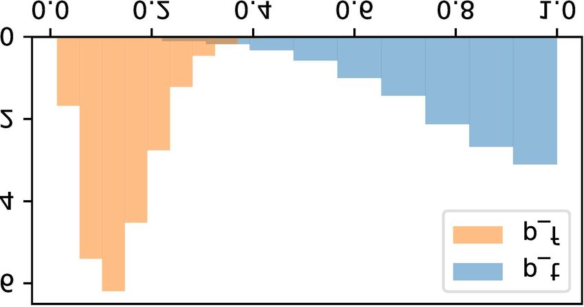
Probabilistic Programs with Stochastic Conditioning

can be expressed as nested probabilistic programs (Rain-         2. Intuition
forth, 2018). However, inference in such programs has lim-
ited choice of algorithms, is computationally expensive, and     To get an intuition behind stochastic conditioning, we take
is difficult to implement correctly (Rainforth et al., 2018).    a fresh look at the Beta-Bernoulli generative model:

In some specific settings, models can be augmented with                    x ∼ Beta(α, β),      y ∼ Bernoulli(x).              (1)
additional auxiliary information, and custom inference tech-
                                                                 The Beta prior on x has α and β parameters, which are inter-
niques can be used. For example, van de Meent et al. (2016)
                                                                 preted as the belief about the number of times y=1 and y=0
employs black-box variational inference on augmented prob-
                                                                 seen before. Since Beta is the conjugate prior for Bernoulli,
abilistic programs for policy search. But problem-specific
                                                                 belief updating in (1) can be performed analytically:
program augmentation and custom inference compromise
the core promise of probabilistic programming: programs                         x|y ∼ Beta(α + y, β + 1 − y)
and algorithms should be separated, and off-the-shelf in-
ference methods should be applicable to a wide range of          We can compose Bayesian belief updating. If after observ-
programs in an automated, black-box manner (Wood et al.,         ing y we observed y ′ , then1
2014; Tolpin, 2019; Winn et al., 2019).
                                                                       x|y ′ ◦ y ∼ Beta(α + y + y ′ , β + 2 − y − y ′ ).
To address these issues and provide a general solution to
defining models and running inference for such problems,         In general, if we observe y1:n = yn ◦ ... ◦ y2 ◦ y1 , then
we propose a way to extend deterministic conditioning                                   Xn                   Xn
p(x|y = y0 ), i.e. conditioning on some random variable             x|y1:n ∼ Beta α +            yi , β + n −           yi .
                                                                                               i=1                   i=1
in our program y taking on a particular value y0 , to stochas-
tic conditioning p(x|y∼D0 ), i.e. conditioning on y having       In (1) (also in many more general exchangeable settings)
the marginal distribution D0 . In the context of a higher-       belief updating is commutative — the posterior distribution
order sampling process in which we first sample a random         does not depend on the order of observations. One may view
probability measure D ∼ p(D) and then sample a ran-              y1:n as a multiset, rather than a sequence, of observations.
dom variable y ∼ D, stochastic conditioning p(x|y∼D0 )           Let us now modify the procedure of presenting the evidence.
amounts to conditioning on the event D = D0 , that is on         Instead of observing the value of each of yn ◦ .... ◦Py2 ◦ y1
the random measure D itself taking the particular form D0 .      in order, we just observe n variates, of which k = i=1 yi
                                                                                                                          n
Equivalently, we can think on conditioning on the event          variates have value 1 (but we are not told which ones). It
y ∼ D0 (based on the first step of our sampling process),        does not matter which of the observations are 1 and which
which says that the marginal distribution of y is given by       are 0. We can even stretch the notion of a single observa-
the distribution D0 . We can develop intuition for this by       tion and say that it is, informally, a ‘combination’ of 1 with
considering the special case of a discrete y, where y ∼ D0       probability θ = nk and 0 with probability 1 − θ. In other
means that the proportion of each possible instance of y         words, we can view each observation yi as an observation of
that occurs will be D0 if we conduct an infinite number of       distribution Bernoulli(θ) itself; the posterior distribution of
rollouts and sample a value of y for each.                       x given n observations of Bernoulli(θ) should be the same
To realize this intuition, we formalize stochastic condition-    as the posterior distribution of x given y1:n . This extended
ing and analyze its properties and usage in the context of       interpretation of belief updating based on observing distri-
probabilistic programming, further showing how effective         butions lets us answer questions about the posterior of x
automated inference engines can be set up for the resulting      given that we observe the distribution Bernoulli(θ) of y:
models. We note that our results also address a basic concep-
                                                                       x| y∼Bernoulli(θ) ∼ Beta(α + θ, β + 1 − θ).
tual problem in Bayesian modeling, and are thus applicable
to non-probabilistic programming settings as well.               Note that observing a distribution does not imply observing
We start with an informal introduction providing intuition       its parametric representation. One may also observe a dis-
about stochastic conditioning (Section 2). Then, we define       tribution through a random source of samples, a black-box
the notion of stochastic conditioning formally and discuss       unnormalized density function, or summary statistics.
its key properties (Section 3), comparing our definition with    Commonly, probabilistic programming involves weighing
possible alternatives and related concepts. Following that,      different assignments to x by the conditional probability of
we discuss efficient inference for programs with stochastic      y given x. For model (1),
conditioning (Section 4). In case studies (Section 5), we
provide probabilistic programs for several problems of sta-                        p(y|x) = xy (1 − x)1−y .
tistical inference which are difficult to approach otherwise,       1
                                                                      By y ′ ◦ y we denote that y ′ was observed after observing y
perform inference on the programs, and analyze the results.      and updating the belief about the distribution of x.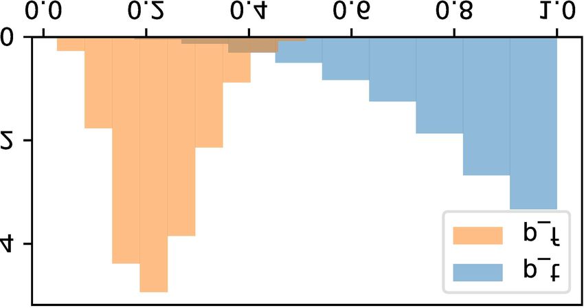
Probabilistic Programs with Stochastic Conditioning
The conditional probability of observing a fixed value ex- An intuition behind the definition can be seen by rewrit-
tends naturally to observing a distribution: ing (3) as a type II geometric integral:
Y
p(y∼Bernoulli(θ)|x) = xθ (1 − x)1−θ p(y∼D|x) = p(y|x)q(y)dy .
Y
= exp (θ log x + (1 − θ) log(1 − x)) (2)
X Definition 2 hence can be interpreted as the probability of
= exp pBern(θ) (y) · log pBern(x) (y) observing all possible draws of y from D, each occurring
y∈{0,1}
according to its probability q(y)dy.
where pBern(r) (y) is the probability mass function of the At this point, the reader may wonder why we do not take the
distribution Bernoulli(r) evaluated at y. Note that pBern(x) following alternative, frequently coming up in discussions:
inside the log is precisely the conditional probability of y Z
in model (1). Equation (2) lets us specify a probabilistic p1 (y∼D|x) = p(y|x) q(y)dy. (4)
program for a version of model (1) with stochastic condi- Y
tioning — on a distribution rather than on a value. In the One may even see a connection between (4) and Jeffrey’s
next section, we introduce stochastic conditioning formally, soft evidence (Jeffrey, 1990)
using a general form of (2). Z
soft
p(x|y ∼D) = q(y)p(x|y) dy, (5)
3. Stochastic Conditioning Y
although the latter addresses a different setting. In soft evi-
Let us define stochastic conditioning formally. In what
dence, an observation is a single value y, but the observer
follows, we mostly discuss the continuous case where the
does not know with certainty which of the values was ob-
observed distribution D has a density q. For the case that
served. Any value y from Y , the domain of D, can be
D does not have a density, the notation q(y)dy in our dis- soft
cussion should be replaced with D(dy), which means the observed with probability q(y), but p(y ∼D|x) cannot be
Lebesgue integral with respect to the distribution (or prob- generally defined (Chan & Darwiche, 2003; Ben Mrad et al.,
ability measure) D. For the discrete case, probability den- 2013). In our setting, distribution D is observed, and the
sities should be replaced with probability masses, and in- observation is certain.
tegrals with sums. Modulo these changes, all the theorem We have two reasons to prefer (3) to (4). First, as Propo-
and propositions in this section carry over to the discrete sition 1 will explain, our p(y∼D|x) is closely related to
case. A general measure-theoretic formalization of stochas- the KL divergence between q(y) and p(y|x), while the al-
tic conditioning, which covers all of these cases uniformly, ternative p1 (y∼D|x) in (4) lacks such connection. The
is described in Appendix A. connection helps understand how p(y∼D|x) alters the prior
Definition 1. A probabilistic model with stochastic condi- of x. Second, p(y∼D|x) treats all possible draws of y
tioning is a tuple (p(x, y), D) where (i) p(x, y) is the joint more equally than p1 (y∼D|x) in the following sense. Both
probability density of random variable x and observation p(y∼D|x) and p1 (y∼D|x) are instances of so called power
y, and it is factored into the product of the prior p(x) and mean (Bullen, 2003) defined by
the likelihood p(y|x) (i.e., p(x, y) = p(x)p(y|x)); (ii) D Z α1
is the distribution from which observation y is marginally pα (y∼D|x) = p(y|x)α q(y)dy . (6)
sampled, and it has a density q(y). Y
Unlike in the usual setting, our objective is to infer Setting α to 0 and 1 gives our p(y∼D|x) and the alternative
p(x|y∼D), the distribution of x given distribution D, rather p1 (y∼D|x), respectively. A general property of this power
than an individual observation y. To accomplish this objec- mean is that as α tends to ∞, draws of y with large p(y|x)
tive, we need to be able to compute p(x, y∼D), a possibly contribute more to pα (y∼D|x), and the opposite situation
unnormalized density on x and distribution D. We define happens as α tends to −∞. Thus, the α = 0 case, which
p(x, y∼D) = p(x)p(y∼D|x) where p(y∼D|x) is the fol- gives our p(y∼D|x), can be regarded as the option that is
lowing unnormalized conditional density: the least sensitive to p(y|x).
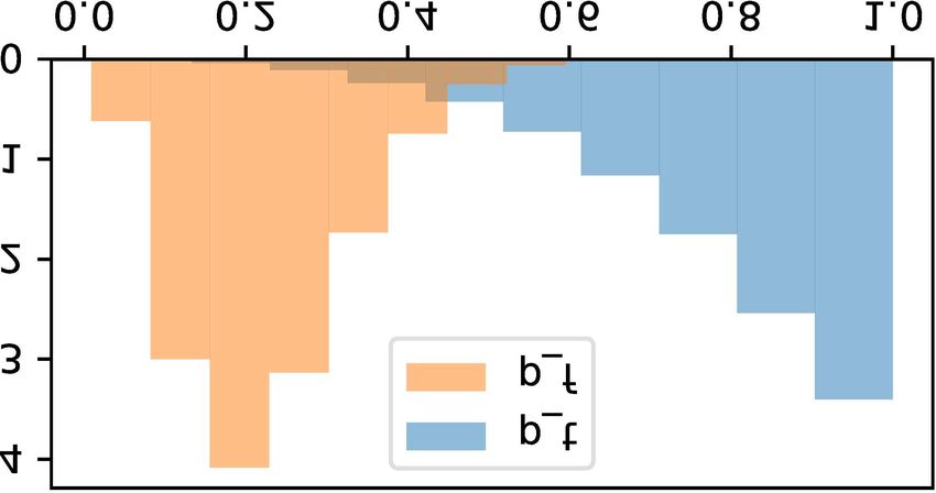
Definition 2. The (unnormalized) conditional density As an illustration of difference between the two definitions,
p(y∼D|x) of D given x is consider Figure 1 showing posteriors of x for the Beta-
Bernoulli model (Section 2) after 1, 5, and 25 observations
of Bernoulli(θ = 0.75), according to either (3) or (4). Ac-
Z
p(y∼D|x) = exp (log p(y|x)) q(y)dy (3) cording to (3) the mode is between 0.5 and 0.75, approach-
Y
ing 0.75 as the number of observations grows; according to
where q is the density of D. the mode is always 1.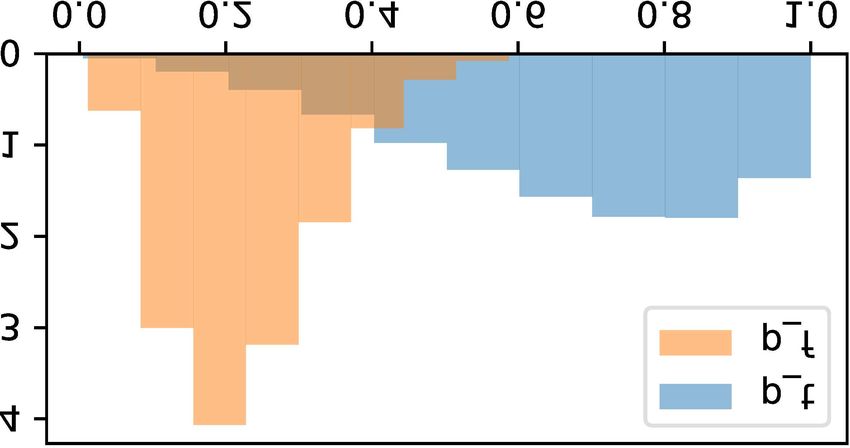
Probabilistic Programs with Stochastic Conditioning
                                                                               Z Z
                                                                           =           p(y|x) qθ (y)dydθ
                                                                               ZΘ Z Y

                                                                             2
                                                                           =              qθ (y) dθ p(y|x)dy
       (a) Definition (3)             (b) Definition (4)                       Y ZΘ                   Z
                                                                                                 ′
Figure 1: Comparison of definitions (3) and (4) on the dis-                ≤ sup          qθ (y ) dθ ·       p(y|x)dy
                                                                                y ′ ∈Y Θ                   Y
crete case of Beta-Bernoulli model (Section 2).                                      Z
                                                                           = sup        qθ (y ′ ) dθ
Probabilistic Programs with Stochastic Conditioning
Another setting in which an unbiased Monte Carlo estimate of the joint probability that they compute than in terms of
of log likelihood is available is subsampling for inference distributions from which x is drawn and y is observed. In
in models with tall data (Korattikara et al., 2014; Bardenet that case, we put the expression for the joint probability
et al., 2014; 2017; Maclaurin & Adams, 2014; Quiroz et al., p(x, y) under the rule, as in (13).
2018; 2019; Dang et al., 2019). In models considered for
subsampling, K observations y1 , y2 , ..., yK are condition- y∼D
y∼D
ally independent given x: x ∼ Prior (12) (13)
p(x, y) = ...
YK y|x ∼ Conditional(x)
p(y1 , y2 , ..., yK |x) = p(yi |x) (10) The code and data for the case studies are provided
i=1
in repository https://bitbucket.org/dtolpin/
Most inference algorithms require evaluation of likelihood
stochastic-conditioning.
p(y1 , y2 , ..., yK |x), which is expensive if K is large. For
example, in importance sampling, the likelihood is in-
5.1. Inferring the Accuracy of Weather Forecast
volved in the computation of importance weights. In many
Markov chain Monte Carlo methods, the ratio of likeli- A person commutes to work either by motorcycle or, on
hoods of the proposed and the current state is a factor in rainy days, by taxi. When the weather is good, the motor-
the Metropolis-Hastings acceptance rate. Subsampling re- cycle ride takes 15 ± 2 minutes via a highway. If rain is
places p(y1 , y2 , ..., yK |x) by an estimate based on N sam- expected, the commuter takes a taxi, and the trip takes 30±4
ples yi1 , yi2 , ..., yiN , N < K, which results in an unbiased minutes, because of crowded roads which slow down a four-
Monte Carlo estimate of log likelihood: wheeled vehicle. Sometimes, however, the rain catches the
commuter in the saddle, and the commuter rides slowly and
K XN
log p(y1 , y2 , ..., yK |x) ≈ log p(yij |x) (11) carefully through rural roads, arriving at 60 ± 8 minutes.
N j=1
Given weather observations and trip durations, we want to
The only difference between (9) and (11) is in factor K, estimate the accuracy of rain forecasts, that is, the probabil-
and inference algorithms for subsampling can be applied to ity of the positive forecast on rainy days pt (true positive)
stochastic conditioning with minor modifications. and on dry days pf (false positive).
A simple bias-adjusted likelihood estimate p̂(x, y∼D), re- The problem is represented by the following model:
quired for the computation of the weights in importance
pr , pt , pf ∼ Beta(1, 1)
sampling as well as of the acceptance ratio in pseudo-
marginal Markov chain Monte Carlo (Andrieu & Roberts, rain|pr ∼ Bernoulli(pr ) (14)
(
2009), can be computed based on (9) (Ceperley & Dewing, Bernoulli(pt ) if rain
1999; Nicholls et al., 2012; Quiroz et al., 2018). Stochastic willRain|pt , pf , rain ∼
Bernoulli(pf ) otherwise
gradient-based inference algorithms (Chen et al., 2014; Ma
et al., 2015; Hoffman et al., 2013; Ranganath et al., 2014; Normal(30, 4) if willRain
Kucukelbir et al., 2017) rely on an unbiased estimate of the duration|rain, willRain ∼ Normal(15, 2) if ¬rain
gradient of log likelihood, which is trivially obtained by
Normal(60, 8) otherwise
differentiating both sides of (9).
Model (14) can be interpreted as either a simulator that
We implemented inference in probabilistic programs with
draws samples of (rain, duration) given pr , pt , and pf , or
stochastic conditioning for Infergo (Tolpin, 2019). To facili-
as a procedure that computes the conditional probability of
tate support for stochastic conditioning in other probabilis-
(rain, duration) given pr , pt , and pf . We use the simulator
tic programming systems, we provide details on likelihood
interpretation to generate synthetic observations for 30 days
estimation and some possible adaptations of inference al-
and pr = 0.2, pt = 0.8, pf = 0.1. The conditional probabil-
gorithms to stochastic conditioning, as well as pointers to
ity interpretation lets us write down a probabilistic program
alternative adaptations in the context of subsampling, in
for posterior inference of pt and pf given observations.
Appendix B.
If, instead of observing (rain, duration) simultaneously, we
5. Case Studies observe weather conditions and trip durations separately
and do not know correspondence between them (a common
In the case studies, we explore several problems cast as situation when measurements are collected by different par-
probabilistic programs with stochastic conditioning. We ties), we can still write a conventional probabilistic program
place y ∼ D above a rule to denote that distribution D is conditioned on the Cartesian product of weather conditions
observed through y and is otherwise unknown to the model, and trip durations, but the number of observations and, thus,
as in (12). Some models are more natural to express in terms time complexity of inference becomes quadratic in the num-Probabilistic Programs with Stochastic Conditioning
Table 1: Summary statistics for populations of municipali-
ties in New York State in 1960; all 804 municipalities and
two random samples of 100. From Rubin (1983).
Population Sample 1 Sample 2
(a) deterministic (b) averaged total 13,776,663 1,966,745 3,850,502
mean 17,135 19,667 38,505
sd 139,147 142,218 228,625
lowest 19 164 162
5% 336 308 315
25% 800 891 863
median 1,668 2,081 1,740
(c) stochastic (d) intensity 75% 5,050 6,049 5,239
95% 30,295 25,130 41,718
Figure 2: Commute to work: posteriors of pt and pf for
highest 2,627,319 1,424,815 1809578
each of the four models. Despite being exposed to partial
information only, models with stochastic conditioning let us
infer informative posteriors.
duration slowed down by rain is supposed to come from a
distribution conditioned on rain intensity.
ber of days. In general, when a model is conditioned on
the Cartesian product of separately obtained observation 5.2. Estimating the Population of New York State
sets, inference complexity grows exponentially with the di-
mensionality of observations, and inference is infeasible in This case study is inspired by Rubin (1983), also appearing
problems with more than a couple of observed features. as Section 7.6 in Gelman et al. (2013). The original case
study evaluated Bayesian inference on the problem of es-
Alternatively, we can draw rain and duration from the obser- timating the total population of 804 municipalities of New
vation sets randomly and independently, and stochastically York state based on a sample of 100 municipalities. Two
condition on D = Rains × Durations: samples were given, with different summary statistics, and
rain, duration ∼ Rains × Durations power-transformed normal model was fit to the data to make
(15) predictions consistent among the samples. The authors of
... the original study apparently had access to the full data set
One can argue that the probabilistic program for the case of (population of each of 804 municipalities). However, only
independent sets of observations of rain and duration can summary description of the samples appears in the publica-
still be implemented with linear complexity by noting that tion: mean, standard deviation, and quantiles (Table 1). We
the domain of rain contains only two values, true and false, show how such summary description can be used to perform
and analytically averaging the evidence over rain. How- Bayesian inference, with the help of stochastic conditioning.
ever, such averaging is often impossible. Consider a variant The original case study in Rubin (1983) started with compar-
of the problem in which the duration of a motorcycle trip ing normal and log-normal models, and finally fit a truncated
in rain depends on rain intensity. Stochastic conditioning, three-parameter power-transformed normal distribution to
along with inference algorithms that use a small number of the data, which helped reconcile conclusions based on each
samples to estimate the log likelihood (magnitude or gra- of the samples while producing results consistent with the
dient), lets us preserve linear complexity in the number of total population. Here, we use a model with log-normal sam-
observations (Doucet et al., 2015; Bardenet et al., 2017). pling distribution, the normal prior on the mean, based on
We fit the model using stochastic gradient Hamiltonian the summary statistics, and the improper uniform prior on
Monte Carlo and used 10 000 samples to approximate the the log of the variance. To complete the model, we stochas-
posterior. Figure 2 shows marginal posteriors of pt and pf tically condition on the piecewise-uniform distribution D of
for each of the four models, on the same simulated data set. municipality populations according to the quantiles:
Posterior distributions should be the same for the analyt-
ically averaged and stochastic models. The deterministic y1...n ∼ Quantiles
model is exposed to more information (correspondence be- √
tween rain occurrence and trip duration). Hence, the poste- m ∼ Normal mean, sd / n , log s2 ∼ Uniform(−∞,∞)
rior distributions are more sharply peaked. The stochastic p
σ = log (s2 /m2 + 1), µ = log m − σ 2 /2 (16)
model with observation of intensity should be less confident
about pt , since now the observation of a motorcycle trip y1...n |m, s2 ∼ LogNormal(µ, σ)Probabilistic Programs with Stochastic Conditioning
in 8 directions (legs) to adjacent squares (Figure 4a). The
unit distance cost of movement depends on the wind (Fig-
ure 4b), which can also blow in 8 directions. There are five
relative boat and wind directions and associated costs: into,
up, cross, down, and away. The cost of sailing into the wind
is prohibitively high, upwind is the highest feasible, and
away from the wind is the lowest. The side of the boat off
which the sail is hanging is called the tack. When the angle
between the boat and the wind changes sign, the sail must
Figure 3: Estimating the population of NY state. 95% be tacked to the opposite tack, which incurs an additional
intervals inferred from the summary statistics include the tacking delay cost. The objective is to find a policy that
true total, and are tighter than Rubin’s results. minimizes the expected travel cost. The wind is assumed to
follow a random walk, either staying the same or switching
to an adjacent direction, with a known probability.
For any given lake size, the optimal policy can be found
using value iteration (Bellman, 1957). The optimal policy
is non-parametric: it tabulates the leg for each combination
of location, tack, and wind. In this case study, we learn a
simple parametric policy, which chooses a leg that maxi-
mizes the sum of the leg cost and the remaining travel cost
after the leg, estimated as the Euclidean distance to the goal
multiplied by the average unit distance cost:
(a) lake (b) points of sail
leg = arg min leg cost(tack , leg, wind )+
(17)
Figure 4: The sailing problem unit-cost · distance(next-location, goal )
The average unit distance cost is the policy variable which
As in Section 5.1, we fit the model using stochastic gradient we infer. Model (18) formalizes our setting. Stochastic con-
HMC and used 10 000 samples to approximate the poste- ditioning on D = RandomWalk models non-determinism
rior. We then used 10 000 draws with replacement of 804- in wind directions.
element sample sets from the predictive posterior to estimate
the total population. The posterior predictive distributions of wind -history ∼ RandomWalk
the total population from both samples are shown in Figure 3. p(wind -history, unit-cost) =
The 95% intervals inferred from the summary statistics, (18)
1 −travel -cost(wind -history, unit-cost)
[9.6×10⁶ , 17.2×10⁶ ] for sample 1, [12.1×10⁶ , 28.1×10⁶ ] exp
Z lake-size · temperature
for sample 2, cover the true total 13.8 × 10⁶ , and are tighter
than the best intervals based on the full samples reported Under policy (17), the boat trajectory and the travel cost are
by Rubin (1983), [6 × 10⁶ , 20 × 106 ] for sample 1 and determined by the wind history and the unit cost. The joint
[10 × 106 , 34 × 106 ] for sample 2. probability of the wind history and the unit cost is given
by the Boltzmann distribution of trajectories with the travel
5.3. The Sailing Problem cost as the energy, a common physics-inspired choice in
stochastic control and policy search (Kappen, 2007; Wingate
The sailing problem (Figure 4) is a popular benchmark prob-
et al., 2011a; van de Meent et al., 2016). The temperature is
lem for search and planning (Péret & Garcia, 2004; Kocsis
a model parameter: the lower the temperature is, the tighter
& Szepesvári, 2006; Tolpin & Shimony, 2012). A sailing
is the concentration of policies around the optimal policy.
boat must travel between the opposite corners A and B of a
A uniform prior on the unit cost, within a feasible range, is
square lake of a given size. At each step, the boat can head
implicitly assumed. If desirable, an informative prior can be
added as a factor depending on the unit cost.
Table 2: Sailing problem parameters The model parameters (cost and wind change probabilities),
same as in Kocsis & Szepesvári (2006); Tolpin & Shimony
cost wind probability (2012), are shown in Table 2. We fit the model using pseudo-
into up cross down away delay same left right marginal Metropolis-Hastings (Andrieu & Roberts, 2009)
∞ 4 3 2 1 4 0.4 0.3 0.3 and used 10 000 samples to approximate the posterior. TheProbabilistic Programs with Stochastic Conditioning
Table 3: Stochastic vs. nested conditioning
model stochastic nested
time evaluations time evaluations
commute 4.1s 2 · 105 520s 4 · 107
nypopu 34s 1 · 107 280s 3 · 108
sailing 5.5s 4 · 105 45s 4 · 106
(a) unit cost
2. A model with nested conditioning is not differentiable
even if latent variables are continuous. Gradient-based
inference algorithms cannot be used, which leaves us
with slow mixing.
As one can see from the comparison in Table 3, implement-
ing the models as probabilistic programs with nested, rather
(b) expected travel cost than stochastic, conditioning results in much slower infer-
Figure 5: The sailing problem. The optimum unit cost is ence.
≈ 3.5–3.9. The dashed lines are the expected travel costs
of the optimal policies, dotted — of the greedy policy. 6. Related Work
Works related to this research belong to several intercon-
nected areas: non-determinism in probabilistic programs,
inferred unit and expected travel costs are shown in Figure 5. nesting of probabilistic programs, inference in nested statis-
Figure 5a shows the posterior distribution of the unit cost, tical models, and conditioning on distributions.
for two temperatures. For all lake sizes in the experiment
(25, 50, 100), the optimal unit cost, corresponding to the Stochastic conditioning can be viewed as an expression of
mode of the posterior, is ≈ 3.5–3.9. Distributions for lower non-determinism with regard to the observed variate. The
temperatures are tighter around the mode. Figure 5b shows problem of representing and handling non-determinism in
the expected travel costs, with the expectations estimated probabilistic programs was raised in Gordon et al. (2014),
both over the unit cost and the wind. The 95% posterior as an avenue for future work. Non-determinism arises, in
intervals are shaded. The inferred travel costs are compared particular, in application of probabilistic programming to
to the travel costs of the optimal policy (the dashed line of policy search in stochastic domains. van de Meent et al.
the same color) and of the greedy policy (the dotted line of (2016) introduce a policy-search specific model specifica-
the same color), according to which the boat always heads tion and inference scheme based on black-box variational
in the direction of the steepest decrease of the distance to the inference. We suggest, and show in a case study, that policy
goal. One can see that the inferred policies attain a lower search in stochastic domains can be cast as inference in
expected travel cost than the greedy policy and become probabilistic programs with stochastic conditioning.
closer to the optimal policy as the temperature decreases. It was noted that probabilistic programs, or queries, can be
nested, and that nested probabilistic programs are able to
5.4. Comparison to nested conditioning represent models beyond those representable by flat proba-
We implemented and evaluated nested conditioning models bilistic programs. Stuhlmüller & Goodman (2014) describe
for each of the case studies. Table 3 compares the running how probabilistic programs can represent nested condition-
times and the number of evaluations of the conditional prob- ing as a part of the model, with examples in diverse areas
ability to reach the effective sample size of 1000 samples. of game theory, artificial intelligence, and linguistics. Sea-
Nested conditioning requires explicit manual coding in the man et al. (2018) apply nested probabilistic programs to
current probabilistic programming frameworks. Inference reasoning about autonomous agents. Some probabilistic
in the presence of nested conditioning is inferior for two programming languages such as Church (Goodman et al.,
reasons: 2008), WebPPL (Goodman & Stuhlmüller, 2014), Angli-
can (Tolpin et al., 2016), and Gen (Cusumano-Towner et al.,
√ 2019) support nesting of probabilistic programs. Stochas-
1. Nested MC estimation requires ≈ N inner samples tic conditioning can be, in principle, represented through
for N outer samples, for each stochastically condi- nesting, however nesting in general incurs difficulties in in-
tioned variable. ference (Rainforth et al., 2018; Rainforth, 2018). StochasticProbabilistic Programs with Stochastic Conditioning
conditioning, introduced in this work, allows both simpler work opens up a wide array of new research directions be-
specification and more efficient inference, eliminating the cause of this. Support for stochastic conditioning in other
need for nesting in many important cases. existing probabilistic programming languages and libraries
is a direction for future work. While we provide a reference
Conditioning of statistical models on distributions or dis-
implementation, used in the case studies, we believe that
tributional properties is broadly used in machine learn-
stochastic conditioning should eventually become a part of
ing (Chen & Gopinath, 2001; Kingma & Welling, 2019;
most probabilistic programming frameworks, just like other
Goodfellow et al., 2014; Makhzani et al., 2015; Bingham
common core concepts.
et al., 2019). Conditioning on distributions represented by
samples is related to subsampling in deep probabilistic pro-
gramming (Tran et al., 2017; TensorFlow, 2018; Bingham Acknowledgments
et al., 2019). Subsampling used with stochastic variational
Yuan Zhou is partially supported by the National Natural
inference (Ranganath et al., 2014) can be interpreted as a
Science Foundation of China (NSFC). Tom Rainforth’s re-
special case of stochastic conditioning. Tavares et al. (2019)
search leading to these results has received funding from
approach the problem of conditioning on distributions by ex-
the European Research Council under the European Union’s
tending probabilistic programming language O MEGA with
Seventh Framework Programme (FP7/2007- 2013)/ ERC
constructs for conditioning on distributional properties such
grant agreement no. 617071. Tom Rainforth was also sup-
as expectation or variance. This work takes a different ap-
ported in part by Junior Research Fellowship from Christ
proach by generalizing deterministic conditioning on values
Church, University of Oxford, and and in part by EP-
to stochastic conditioning on distributions, without the need
SRC funding under grant EP/P026753/1. Hongseok Yang
to explicitly compute or estimate particular distributional
was supported by the Engineering Research Center Pro-
properties, and leverages inference algorithms developed in
gram through the National Research Foundation of Korea
the context of subsampling (Korattikara et al., 2014; Bar-
(NRF) funded by the Korean Government MSIT (NRF-
denet et al., 2014; 2017; Maclaurin & Adams, 2014; Quiroz
2018R1A5A1059921), and also by Next-Generation Infor-
et al., 2018; 2019; Dang et al., 2019) for efficient inference
mation Computing Development Program through the Na-
in probabilistic programs with stochastic conditioning.
tional Research Foundation of Korea (NRF) funded by the
There is a connection between stochastic conditioning and Ministry of Science, ICT (2017M3C4A7068177). We thank
Jeffrey’s soft evidence (Jeffrey, 1990). In soft evidence, the PUB+ for supporting development of Infergo.
observation is uncertain; any one out of a set of observations
could have been observed with a certain known probabil- References
ity. A related concept in the context of belief networks is
virtual evidence (Pearl, 1988). Chan & Darwiche (2003) Andrieu, C. and Roberts, G. O. The pseudo-marginal ap-
demonstrate that Jeffrey’s soft evidence and Pearl’s virtual proach for efficient Monte Carlo computations. The An-
evidence are different formulations of the same concept. nals of Statistics, 37(2):697–725, 2009.
Ben Mrad et al. (2013); Dietrich et al. (2016); Jacobs (2018)
elaborate on connection between soft and virtual evidence Bardenet, R., Doucet, A., and Holmes, C. Towards scaling
and their role in probabilistic inference. In probabilistic up Markov chain Monte Carlo: an adaptive subsampling
programming, some cases of soft conditioning (Wood et al., approach. In Proceedings of the 31st International Con-
2014; Goodman & Stuhlmüller, 2014) can be interpreted ference on Machine Learning, pp. 405–413, 2014.
as soft evidence. In this work, the setting is different: a Bardenet, R., Doucet, A., and Holmes, C. On Markov chain
distribution is observed, and the observation is certain. Monte Carlo methods for tall data. Journal of Machine
Learning Research, 18(47):1–43, 2017.
7. Discussion
Bellman, R. A Markovian decision process. Journal of
In this work, we introduced the notion of stochastic condi- Mathematics and Mechanics, 6(5):679–684, 1957.
tioning. We described kinds of problems for which deter-
ministic conditioning is insufficient, and showed on case Ben Mrad, A., Delcroix, V., Piechowiak, S., Maalej, M. A.,
studies how probabilistic programs with stochastic condi- and Abid, M. Understanding soft evidence as probabilis-
tioning can be used to represent and efficiently analyze such tic evidence: Illustration with several use cases. In 2013
problems. We believe that adoption of stochastic condition- 5th International Conference on Modeling, Simulation
ing in probabilistic programming frameworks will facilitate and Applied Optimization (ICMSAO), pp. 1–6, 2013.
convenient modeling of new classes of problems, while Bingham, E., Chen, J. P., Jankowiak, M., Obermeyer, F.,
still supporting robust and efficient inference. The idea of Pradhan, N., Karaletsos, T., Singh, R., Szerlip, P., Hors-
stochastic conditioning is very general, and we believe our fall, P., and Goodman, N. D. Pyro: deep universal prob-Probabilistic Programs with Stochastic Conditioning
abilistic programming. Journal of Machine Learning Ghosal, S. and van der Vaart, A. Fundamentals of Nonpara-
Research, 20(28):1–6, 2019. metric Bayesian Inference. Cambridge Series in Statisti-
cal and Probabilistic Mathematics. Cambridge University
Bullen, P. S. Handbook of Means and Their Inequalities. Press, 2017. doi: 10.1017/9781139029834.
Springer Netherlands, 2003.
Goodfellow, I., Pouget-Abadie, J., Mirza, M., Xu, B.,
Carpenter, B., Gelman, A., Hoffman, M., Lee, D., Goodrich,
Warde-Farley, D., Ozair, S., Courville, A., and Bengio,
B., Betancourt, M., Brubaker, M., Guo, J., Li, P., and
Y. Generative adversarial nets. In Advances in Neural
Riddell, A. Stan: a probabilistic programming lan-
Information Processing Systems, pp. 2672–2680. 2014.
guage. Journal of Statistical Software, Articles, 76(1):
1–32, 2017. Goodman, N. D. and Stuhlmüller, A. The Design and Im-
plementation of Probabilistic Programming Languages.
Ceperley, D. M. and Dewing, M. The penalty method for
2014. URL http://dippl.org/. electronic; re-
random walks with uncertain energies. The Journal of
trieved 2019/3/29.
Chemical Physics, 110(20):9812–9820, May 1999.
Chan, H. and Darwiche, A. On the revision of probabilistic Goodman, N. D., Mansinghka, V. K., Roy, D. M., Bonawitz,
beliefs using uncertain evidence. Artificial Intelligence, K., and Tenenbaum, J. B. Church: a language for genera-
163:67–90, 2003. tive models. In Proceedings of the 24th Conference on
Uncertainty in Artificial Intelligence, pp. 220–229, 2008.
Chen, S. S. and Gopinath, R. A. Gaussianization. In Ad-
vances in Neural Information Processing Systems, pp. Gordon, A. D., Henzinger, T. A., Nori, A. V., and Rajamani,
423–429. 2001. S. K. Probabilistic programming. In Proceedings of the
36th International Conference on Software Engineering
Chen, T., Fox, E. B., and Guestrin, C. Stochastic gradient (ICSE, FOSE track), pp. 167–181, 2014.
Hamiltonian Monte Carlo. In Proceedings of the 31st
International Conference on on Machine Learning, pp. Hoffman, M. D. and Gelman, A. The No-U-Turn sampler:
1683–1691, 2014. adaptively setting path lengths in Hamiltonian Monte
Carlo. arXiv:1111.4246, 2011.
Cusumano-Towner, M. F., Saad, F. A., Lew, A. K., and
Mansinghka, V. K. Gen: A general-purpose probabilistic Hoffman, M. D., Blei, D. M., Wang, C., and Paisley, J.
programming system with programmable inference. In Stochastic variational inference. Journal of Machine
Proceedings of the 40th ACM SIGPLAN Conference on Learning Research, 14:1303–1347, 2013.
Programming Language Design and Implementation, pp.
221–236, 2019. Jacobs, B. The mathematics of changing one’s mind, via
Jeffrey’s or via Pearl’s update rule. arXiv:1807.05609,
Dang, K.-D., Quiroz, M., Kohn, R., Tran, M.-N., and Villani, 2018.
M. Hamiltonian Monte Carlo with energy conserving
subsampling. Journal of Machine Learning Research, 20 Jeffrey, R. The Logic of Decision. McGraw-Hill series in
(100):1–31, 2019. probability and statistics. University of Chicago Press,
1990.
Dietrich, F., List, C., and Bradley, R. Belief revision gen-
eralized: A joint characterization of Bayes’ and Jeffrey’s Kappen, H. J. An introduction to stochastic control theory,
rules. Journal of Economic Theory, 162:352–371, 2016. path integrals and reinforcement learning. In American
Institute of Physics Conference Series, volume 887, pp.
Doucet, A., Pitt, M. K., Deligiannidis, G., and Kohn, R. 149–181, 2007.
Efficient implementation of Markov chain Monte Carlo
when using an unbiased likelihood estimator. Biometrika, Kim, J. and Pearl, J. A computational model for causal
102(2):295–313, 03 2015. and diagnostic reasoning in inference systems. In Pro-
ceedings of International Joint Conference on Artificial
Ge, H., Xu, K., and Ghahramani, Z. Turing: composable Intelligence, pp. 190–193, 1983.
inference for probabilistic programming. In Proceed-
ings of the 21st Conference on International Conference Kingma, D. P. and Welling, M. An introduction to varia-
on Artificial Intelligence and Statistics, pp. 1682–1690, tional autoencoders. Foundations and Trends in Machine
2018. Learning, 12(4):307–392, 2019.
Gelman, A., Carlin, J., Stern, H., Dunson, D., Vehtari, A., Kocsis, L. and Szepesvári, C. Bandit based Monte-Carlo
and Rubin, D. Bayesian Data Analysis. Chapman & planning. In Proceedings of the European Conference on
Hall/CRC Texts in Statistical Science. CRC Press, 2013. Machine Learning, pp. 282–293, 2006.Probabilistic Programs with Stochastic Conditioning
Korattikara, A., Chen, Y., and Welling, M. Austerity in Ranganath, R., Gerrish, S., and Blei, D. M. Black box
MCMC land: Cutting the Metropolis-Hastings budget. variational inference. In Proceedings of the 17th Confer-
In Proceedings of the 31st International Conference on ence on Artificial Intelligence and Statistics, pp. 814–822,
Machine Learning, pp. 181–189, 2014. 2014.
Kucukelbir, A., Tran, D., Ranganath, R., Gelman, A., and Rubin, D. B. A case study of the robustness of Bayesian
Blei, D. M. Automatic differentiation variational infer- methods of inference: Estimating the total in a finite
ence. Journal of Machine Learning Research, 18(1): population using transformations to normality. In Box,
430–474, January 2017. G., Leonard, T., and Wu, C.-F. (eds.), Scientific Inference,
Data Analysis, and Robustness, pp. 213–244. Academic
Ma, Y.-A., Chen, T., and Fox, E. A complete recipe for Press, 1983.
stochastic gradient MCMC. In Advances in Neural Infor-
mation Processing Systems, pp. 2917–2925. 2015. Seaman, I. R., van de Meent, J.-W., and Wingate, D. Nested
reasoning about autonomous agents using probabilistic
Maclaurin, D. and Adams, R. Firefly Monte Carlo: Exact programs. arXiv:1812.01569, 2018.
MCMC with subsets of data. In Proceedings of the 30th Staton, S., Yang, H., Wood, F., Heunen, C., and Kammar, O.
Conference on Uncertainty in Artificial Intelligence, pp. Semantics for probabilistic programming: Higher-order
543–552, 2014. functions, continuous distributions, and soft constraints.
Makhzani, A., Shlens, J., Jaitly, N., Goodfellow, I., and Frey, In Proceedings of the 31st Annual ACM/IEEE Symposium
B. Adversarial autoencoders. arXiv:1511.05644, 2015. on Logic in Computer Science, pp. 525–534, 2016.
Stuhlmüller, A. and Goodman, N. Reasoning about rea-
Nicholls, G. K., Fox, C., and Watt, A. M. Cou- soning by nested conditioning: Modeling theory of mind
pled MCMC with a randomized acceptance probability. with probabilistic programs. Cognitive Systems Research,
arXiv:1205.6857, 2012. 28:80–99, 2014. Special Issue on Mindreading.
Papadimitriou, C. H. and Yannakakis, M. Shortest paths Tavares, Z., Zhang, X., Minasyan, E., Burroni, J., Ran-
without a map. In Proceedings of 16th International ganath, R., and Lezama, A. S. The random condi-
Colloquium on Automata, Languages and Programming, tional distribution for higher-order probabilistic inference.
pp. 610–620, 1989. arXiv:1903.10556, 2019.
Pearl, J. Probabilistic Reasoning in Intelligent Systems: TensorFlow. TensorFlow probability. https://www.
Networks of Plausible Inference. Morgan Kaufmann tensorflow.org/probability/, 2018.
Publishers Inc., San Francisco, CA, USA, 1988.
Tolpin, D. Deployable probabilistic programming. In Pro-
Péret, L. and Garcia, F. On-line search for solving Markov ceedings of the 2019 ACM SIGPLAN International Sym-
decision processes via heuristic sampling. In Proceed- posium on New Ideas, New Paradigms, and Reflections
ings of the 16th European Conference on Artificial Intel- on Programming and Software, pp. 1–16, 2019.
ligence, pp. 530–534, 2004. Tolpin, D. and Shimony, S. E. MCTS based on simple regret.
Quiroz, M., Villani, M., Kohn, R., Tran, M.-N., and Dang, In Proceedings of The 26th AAAI Conference on Artificial
K.-D. Subsampling mcmc — an introduction for the Intelligence, pp. 570–576, 2012.
survey statistician. Sankhya A, 80(1):33–69, Dec 2018. Tolpin, D., van de Meent, J.-W., Yang, H., and Wood, F. De-
sign and implementation of probabilistic programming
Quiroz, M., Kohn, R., Villani, M., and Tran, M.-N. Speeding language Anglican. In Proceedings of the 28th Sympo-
up MCMC by efficient data subsampling. Journal of sium on the Implementation and Application of Func-
the American Statistical Association, 114(526):831–843, tional Programming Languages, pp. 6:1–6:12, 2016.
2019.
Tran, D., Hoffman, M. D., Saurous, R. A., Brevdo, E., Mur-
Rainforth, T. Nesting probabilistic programs. In Proceed- phy, K., and Blei, D. M. Deep probabilistic programming.
ings of the 34th Conference on Uncertainty in Artificial In Proceedings of the 5th International Conference on
Intelligence, pp. 249–258, 2018. Learning Representations, 2017.
Rainforth, T., Cornish, R., Yang, H., Warrington, A., and van de Meent, J.-W., Paige, B., Tolpin, D., and Wood, F.
Wood, F. On nesting Monte Carlo estimators. In Proceed- Black-box policy search with probabilistic programs. In
ings of the 35th International Conference on Machine Proceedings of the 19th International Conference on Ar-
Learning, pp. 4267–4276, 2018. tificial Intelligence and Statistics, pp. 1195–1204, 2016.Probabilistic Programs with Stochastic Conditioning Wingate, D., Goodman, N. D., Roy, D. M., Kaelbling, L. P., and Tenenbaum, J. B. Bayesian policy search with policy priors. In Proceedings of the 22nd International Joint Conference on Artificial Intelligence, pp. 1565–1570, 2011a. Wingate, D., Stuhlmüller, A., and Goodman, N. D. Lightweight implementations of probabilistic program- ming languages via transformational compilation. In Pro- ceedings of the 14th Conference on Artificial Intelligence and Statistics, pp. 770–778, 2011b. Winn, J., Bishop, C. M., Diethe, T., and Zaykov, Y. Model Based Machine Learning. 2019. URL http: //mbmlbook.com/. electronic; retrieved 2019/4/21. Wood, F., van de Meent, J.-W., and Mansinghka, V. A new approach to probabilistic programming inference. In Proceedings of the 17th International Conference on Ar- tificial Intelligence and Statistics, pp. 1024–1032, 2014.
You can also read