Mean Field Games Flock! The Reinforcement Learning Way
←
→
Page content transcription
If your browser does not render page correctly, please read the page content below
Mean Field Games Flock! The Reinforcement Learning Way
                                                   Sarah Perrin1 , Mathieu Laurière2 , Julien Pérolat3 , Matthieu Geist4 , Romuald
                                                                                Élie3 and Olivier Pietquin4
                                                              1
                                                                Univ. Lille, CNRS, Inria, Centrale Lille, UMR 9189 CRIStAL
                                                                                 2
                                                                                   Princeton University, ORFE
                                                                                        3
                                                                                          DeepMind Paris
                                                                               4
                                                                                 Google Research, Brain Team
                                               sarah.perrin@inria.fr, lauriere@princeton.edu, {perolat, mfgeist, relie, pietquin}@google.com,
arXiv:2105.07933v1 [cs.MA] 17 May 2021

                                                                   Abstract                                 of agents, emphasizing how a consensus can be reached in a
                                                                                                            group without centralized decisions. Such question is often
                                              We present a method enabling a large number of                studied using the notion of Nash equilibrium and becomes
                                              agents to learn how to flock, which is a natural be-          extremely complex when the number of agents grows.
                                              havior observed in large populations of animals.                 A way to approximate Nash equilibria in large games is to
                                              This problem has drawn a lot of interest but re-              study the limit case of an continuum of identical agents, in
                                              quires many structural assumptions and is tractable           which the local effect of each agent becomes negligible. This
                                              only in small dimensions. We phrase this problem              is the basis of the Mean Field Games (MFGs) paradigm intro-
                                              as a Mean Field Game (MFG), where each individ-               duced in [Lasry and Lions, 2007]. MFGs have found numer-
                                              ual chooses its acceleration depending on the pop-            ous applications from economics to energy production and
                                              ulation behavior. Combining Deep Reinforcement                engineering. A canonical example is crowd motion modeling
                                              Learning (RL) and Normalizing Flows (NF), we                  in which pedestrians want to move while avoiding congestion
                                              obtain a tractable solution requiring only very weak          effects. In flocking, the purpose is different since the agents
                                              assumptions. Our algorithm finds a Nash Equilib-              intend to remain together as a group, but the mean-field ap-
                                              rium and the agents adapt their velocity to match             proximation can still be used to mitigate the complexity.
                                              the neighboring flock’s average one. We use Ficti-               However, finding an equilibrium in MFGs is computa-
                                              tious Play and alternate: (1) computing an approxi-           tionally intractable when the state space exceeds a few di-
                                              mate best response with Deep RL, and (2) estimat-             mensions. In traditional flocking models, each agent’s state
                                              ing the next population distribution with NF. We              is described by a position and a velocity, while the con-
                                              show numerically that our algorithm learn multi-              trol is the acceleration. In terms of computational cost, this
                                              group or high-dimensional flocking with obstacles.            typically rules out state-of-the-art numerical techniques for
                                                                                                            MFGs based on finite difference schemes for partial differen-
                                                                                                            tial equations (PDEs) [Achdou and Capuzzo-Dolcetta, 2010].
                                         1   Introduction                                                   In addition, PDEs are in general hard to solve when the ge-
                                         The term flocking describes the behavior of large populations      ometry is complex and require full knowledge of the model.
                                         of birds that fly in compact groups with similar velocities,          For these reasons, Reinforcement Learning (RL) to learn
                                         often exhibiting elegant motion patterns in the sky. Such be-      control strategies for MFGs has recently gained in popular-
                                         havior is pervasive in the animal realm, from fish to birds,       ity [Guo et al., 2019; Elie et al., 2020; Perrin et al., 2020].
                                         bees or ants. This intriguing property has been widely stud-       Combined with deep neural nets, RL has been used success-
                                         ied in the scientific literature [Shaw, 1975; Reynolds, 1987]      fully to tackle problems which are too complex to be solved
                                         and its modeling finds applications in psychology, animation,      by exact methods [Silver et al., 2018] or to address learn-
                                         social science, or swarm robotics. One of the most popu-           ing in multi-agent systems [Lanctot et al., 2017]. Particu-
                                         lar approaches to model flocking was proposed in [Cucker           larly relevant in our context, are works providing techniques
                                         and Smale, 2007] and allows predicting the evolution of each       to compute an optimal policy [Haarnoja et al., 2018; Lilli-
                                         agent’s velocity from the speeds of its neighbors.                 crap et al., 2016] and methods to approximate probability dis-
                                            To go beyond pure description of population behaviours          tributions in high dimension [Rezende and Mohamed, 2015;
                                         and emphasize on the decentralized aspect of the underlying        Kobyzev et al., 2020].
                                         decision making process, this model has been revisited to in-         Our main contributions are: (1) we cast the flocking prob-
                                         tegrate an optimal control perspective, see e.g. [Caponigro et     lem into a MFG and propose variations which allow multi-
                                         al., 2013; Bailo et al., 2018]. Each agent controls its velocity   group flocking as well as flocking in high dimension with
                                         and hence its position by dynamically adapting its accelera-       complex topologies, (2) we introduce the Flock’n RL algo-
                                         tion so as to maximize a reward that depends on the others’        rithm that builds upon the Fictitious Play paradigm and in-
                                         behavior. An important question is a proper understanding          volves deep neural networks and RL to solve the model-free
                                         of the nature of the equilibrium reached by the population         flocking MFG, and (3) we illustrate our approach on several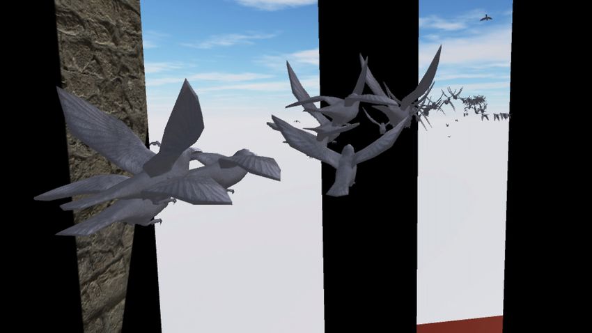
numerical examples and evaluate the solution with approxi-                                        The total payoff of agent i given the other agents’ strate-
mate performance matrix and exploitability.                                                       gies uh−i = (u1 , .i. . , ui−1 , ui+1 , . . . , uN ) is: Fui −i (ui ) =
                                                                                                                  t i             i
                                                                                                            P
                                                                                                  Exit ,vti  t≥0 γ ft , with ft defined Eq. (1). In this context,
2     Background
                                                                                                  a Nash equilibrium is a strategy profile (û1 , û2 , . . . , ûN ) such
Three main formalisms will be combined: flocking, Mean                                            that there’s no profitable unilateral deviation, i.e., for every
Field Games (MFG), Reinforcement Learning (RL).                                                   i = 1, . . . , N , for every control ui , Fûi −i (ûi ) ≥ Fûi −i (ui ).
  Ez stands for the expectation w.r.t. the random variable z.
                                                                                                  2.2    Mean Field Games
2.1    The model of flocking
                                                                                                  An MFG describes a game for a continuum of identical agents
To model a flocking behaviour, we consider the following                                          and is fully characterized by the dynamics and the payoff
system of N agents derived in a discrete time setting in                                          function of a representative agent. More precisely, denoting
[Nourian et al., 2011] from Cucker-Smale flocking modeling.                                       by µt the state distribution of the population, and by ξt ∈ R`
Each agent i has a position and a velocity, each in dimension                                     and αt ∈ Rk the state and the control of an infinitesimal
d and denoted respectively by xi and v i . We assume that it                                      agent, the dynamics of the infinitesimal agent is given by
can control its velocity by choosing the acceleration, denoted
by ui . The dynamics of agent i ∈ {1, . . . , N } is:                                                            ξt+1 = ξt + b(ξt , αt , µt ) + σt+1 ,                (4)
                                                                                                  where b : R` × Rk × P(R` ) → R` is a drift (or transition)
      xit+1   =   xit   +   vti ∆t,          i
                                            vt+1   =   vti   +   uit ∆t   +   it+1 ,             function, σ is a ` × ` matrix and t+1 is a noise term taking
                                                                                                  values in R` . We assume that the sequence of noises (t )t≥0
where ∆t is the time step and it is a random variable playing                                    is i.i.d. (e.g. Gaussian). The objective of each infinitesi-
the role of a random disturbance. We assume that each agent                                       mal agent is to maximize its total expected payoff, defined
is optimizing for a flocking criterion f that is underlying to                                    given a flow of distributions µ = (µt )t≥0 and a strategy α
the flocking behaviour. For agent i at time t, f is of the form:                                  (i.e., a stochastic process adapted
                                                                                                                                  h Pto the filtration generated
                                                                                                                                                            i    by
                                                                                                                                           t
                                                                                                  (t )t≥0 ) as: Jµ (α) = Eξt ,αt     t≥0 γ ϕ(ξt , αt , µt ) , where
                            fti = f (xit , vti , uit , µN
                                                        t ),                               (1)
where the interactions with other agents are only through                                         γ ∈ (0, 1) is a discount factor and ϕ : R` ×Rk ×P(R` ) → R`
the empirical distribution of states and velocities denoted by:                                   is an instantaneous payoff function. Since this payoff de-
       1
         PN                                                                                       pends on the population’s state distribution, and since the
µNt = N     j=1 δ(xjt ,vtj ) .                                                                    other agents would also aim to maximize their payoff, a nat-
   We focus on criteria incorporating a term of the form:                                         ural approach is to generalize the notion of Nash equilibrium
                                                                                      2           to this framework. A mean field (Nash) equilibrium is de-
                                              (v − v 0 )
                                Z
 fβflock (x, v, u, µ) = -                                    dµ(x0 , v 0 )                , (2)   fined as a pair (µ̂, α̂) = (µ̂t , α̂t )t≥0 of a flow of distributions
                                    R2d   (1 + kx − x0 k2 )β                                      and strategies such that the following two conditions are sat-
where β ≥ 0 is a parameter and (x, v, u, µ) ∈ Rd ×Rd ×Rd ×                                        isfied: α̂ is a best response against µ̂ (optimality) and µ̂ is the
P(Rd × Rd ), with P(E) denoting the set of probability mea-                                       distribution generated by α̂ (consistency), i.e.,
sures on a set E. This criterion incentivises agents to align                                       1. α̂ maximizes α 7→ Jµ̂ (α);
their velocities, especially if they are close to each other. Note                                  2. for every t ≥ 0, µ̂t is the distribution of ξt when it fol-
that β parameterizes the level of interactions between agents                                          lows the dynamics (4) with (αt , µt ) replaced by (α̂t , µ̂t ).
and strongly impacts the flocking behavior: if β = 0, each
agent tries to align its velocity with all the other agents of the                                Finding a mean field equilibrium thus amounts to finding a
population irrespective of their positions, whereas the larger                                    fixed point in the space of (flows of) probability distributions.
β > 0, the more importance is given to its closest neighbors                                      The existence of equilibria can be proven through classical
(in terms of position).                                                                           fixed point theorems [Carmona and Delarue, 2018]. In most
   In the N -agent case, for agent i, it becomes:                                                 mean field games considered in the literature, the equilib-
                                                                                                  rium is unique, which can be proved using either a strict con-
                                                                              2
                              N                                                                   traction argument or the so-called Lasry-Lions monotonic-
          flock,i          1 X       (vti − vtj )                                                 ity condition [Lasry and Lions, 2007]. Computing solutions
         fβ,t           =−                                                        .        (3)
                           N j=1 (1 + kxit − xjt k2 )β                                            to MFGs is a challenging task, even when the state is in
                                                                                                  small dimension, due to the coupling between the optimal-
The actual criterion will typically include other terms, for in-                                  ity and the consistency conditions. This coupling typically
stance to discourage agents from using a very large accelera-                                     implies that one needs to solve a forward-backward system
tion, or to encourage them to be close to a specific position.                                    where the forward equation describes the evolution of the
We provide such examples in Sec. 4.                                                               distribution and the backward equation characterizes the op-
   Since the agents may be considered as selfish (they try to                                     timal control. One can not be solved prior to the other one,
maximize their own criterion) and may have conflicting goals                                      which leads to numerical difficulties. The basic approach,
(e.g. different desired velocities), we consider Nash equi-                                       which consists in iteratively solving each equation, works
librium as a notion of solution to this problem and the in-                                       only in very restrictive settings and is otherwise subject to
dividual criterion can be seen as the payoff for each agent.                                      cycles. A method which does not suffer from this limitation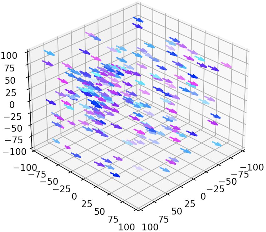
Algorithm 1: Generic Fictitious Play in MFGs                    namely Actor-Critic, which relies on both a representation
                                                                  of the policy and of the so-called state-action value function
   input : MFG = {ξ, ϕ, µ0 }; # of iterations J ;                 (s, a) 7→ Qπ (s, a). Qπ (s, a) is the total return conditioned on
1 Define µ̄0 = µ0 for j = 1, . . . , J do
                                                                  starting in state s and using action a before using policy π for
2    1. Set best response αj = arg maxα Jµ̄j−1 (α) and            subsequent time steps. It can be estimated by bootstrapping,
        let ᾱj be the average of (αi )i=0,...,j                  using the Markov property, through the Bellman equations.
3    2. Set µj = γ-stationary distribution induced by αj          Most recent implementations rely on deep neural networks to
4    3. Set µ̄j = j−1          1
                     j µ̄j−1 + j µj                               approximate π and Q (e.g. [Haarnoja et al., 2018]).
5 return ᾱJ , µ̄J

                                                                  3     Our approach
                                                                  In this section, we put together the pieces of the puzzle to
is Fictitious Play, summarized in Alg. 1. It consists in com-     numerically solve the flocking model. Based on a mean-field
puting the best response against a weighted average of past       approximation, we first recast the flocking model as an MFG
distributions instead of just the last distribution. This algo-   with decentralized decision making, for which we propose a
rithm has been shown to converge for more general MFGs.           numerical method relying on RL and deep neural networks.
State-of-the-art numerical methods for MFGs based on par-
tial differential equations can solve such problems with a high   3.1    Flocking as an MFG
precision when the state is in small dimension and the ge-
ometry is elementary [Achdou and Capuzzo-Dolcetta, 2010;          Mean field limit. We go back to the model of flocking
Carlini and Silva, 2014]. More recently, numerical methods        introduced in Sec. 2.1. When the number of agents grows to
based on machine learning tools have been developed [Car-         infinity, the empirical distribution µN
                                                                                                        t is expected to converge
mona and Laurière, 2019; Ruthotto et al., 2020]. These tech-     towards the law µt of (xt , vt ), which represents the position
niques rely on the full knowledge of the model and are re-        and velocity of an infinitesimal agent and have dynamics:
stricted to classes of quite simple MFGs.                               xt+1 = xt + vt ∆t,         vt+1 = vt + ut ∆t + t+1 .
2.3   Reinforcement Learning                                      This problem can be viewed as an instance of the MFG frame-
The Reinforcement Learning (RL) paradigm is the machine           work discussed in Sec. 2.2, by taking the state to be the
learning answer to the optimal control problem. It aims at        position-velocity pair and the action to be the acceleration,
learning an optimal policy for an agent that interacts in an      i.e., the dimensions are ` = 2d, k = d, and ξ = (x, v), α = u.
environment composed of states, by performing actions. For-       To accommodate for the degeneracy of         the noise
                                                                                                                        as only the
mally, the problem is framed under the Markov Decision Pro-                                                     0d 0d
                                                                  velocities are disturbed, we take σ =                    where 1d is
cesses (MDP) framework. An MDP is a tuple (S, A, p, r, γ)                                                       0d 1d
where S is a state space, A is an action space, p : S × A →       the d-dimensional identity matrix.
P(S) is a transition kernel, r : S × A → R is a reward               The counterpart of the notion of N -agent Nash equilib-
function and γ is a discount factor (see Eq. (5)). Using ac-      rium is an MFG equilibrium as described in Sec. 2.2. We
tion a when the current state is s leads to a new state dis-      focus here on equilibria which are stationary in time. In
tributed according to P (s, a) and produces a reward R(s, a).     other words, the goal is to find a pair (µ̂, û) where µ̂ ∈
A policy π : S → P(A), s 7→ π(·|s) provides a distribu-           P(R` × R` ) is a position-velocity distribution and û : R` ×
tion over actions for each state. RL aims at learning a policy    R` 7→ R` is a feedback function to determine the accel-
π ∗ which maximizes the total return defined as the expected      eration given the position and velocity, such that: (1) µ̂ is
(discounted) sum of future rewards:                               an invariant position-velocity distribution if the whole pop-
                               hX                  i              ulation uses the acceleration given by û, and (2) û maxi-
             R(π) = Eat ,st+1       γ t r(st , at ) ,      (5)    mizes the rewards when the agent’s initial position-velocity
                                t≥0                               distribution is µ̂ and the population distribution is µ̂ at ev-
with at ∼ π(·|st ) and st+1 ∼ p(·|st , at ). Note that if the
                                                                  ery time hstep. In mathematical terms,   i û maximizes Jµ̂ (u) =
                                                                                      t
                                                                              P
dynamics (p and r) is known to the agent, the problem can         Ext ,vt ,ut    t≥0 γ ϕ(xt , vt , ut , µ̂) , where (xt , vt )t≥0 is the
be solved using e.g. dynamic programming. Most of the             trajectory of an infinitesimal agent who starts with distribu-
time, these quantities are unknown and RL is required. A          tion µ̂ at time t = 0 and is controlled by the acceleration
plethora of algorithms exist to address the RL problem. Yet,      (ut )t≥0 . As the payoff function ϕ we use fβflock from Eq. (2).
we need to focus on methods that allow continuous action          Moreover, the consistency condition rewrites as: µ̂ is the sta-
spaces as we want to control accelerations. One category of       tionary distribution of (xt , vt )t≥0 if controlled by (ût )t≥0 .
such algorithms is based on the Policy Gradient (PG) theo-           Theoretical analysis. The analysis of MFG with flock-
rem [Sutton et al., 1999] and makes use of the gradient as-       ing effects is challenging due to the unusual structure of the
cent principle: π ← π + α ∂R(π)  ∂π , where α is a learning       dynamics and the payoff, which encourages gathering of the
rate. Yet, PG methods are known to be high-variance be-           population. This is running counter to the classical Lasry-
cause they use Monte Carlo rollouts to estimate the gradi-        Lions monotonicity condition [Lasry and Lions, 2007], which
ent. A vast literature thus addresses the variance reduction      typically penalizes the agents for being too close to each
problem. Most of the time, it involves an hybrid architecture,    other. However, existence and uniqueness have been proved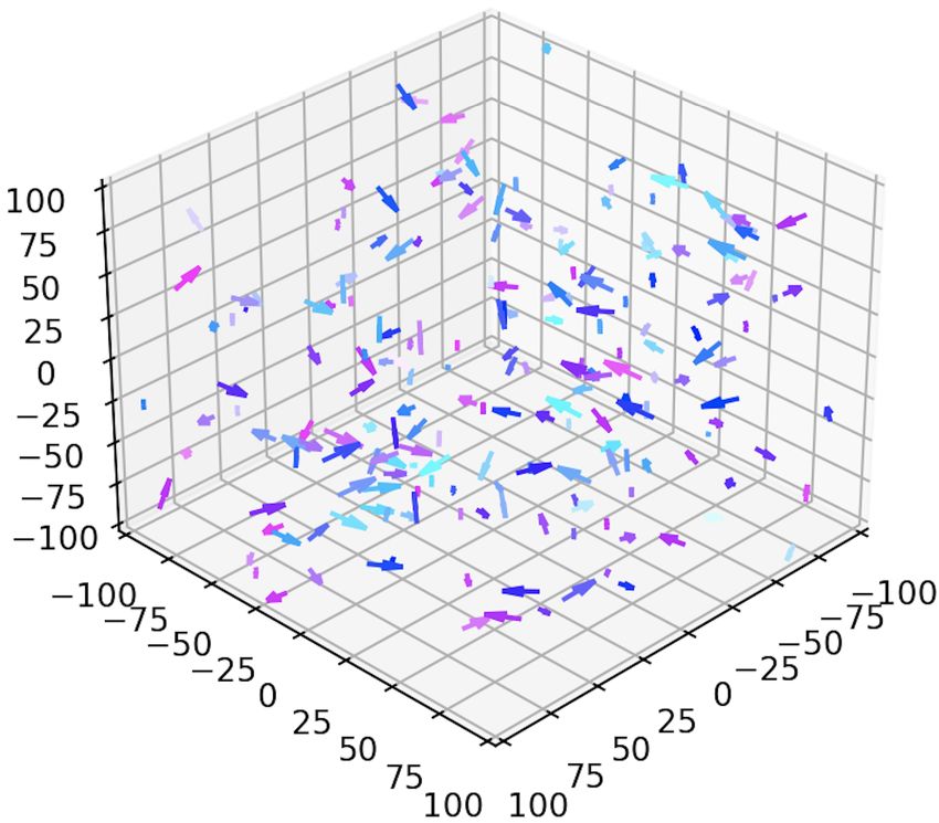
Algorithm 2: Flock’n RL                                        to work on continuous action spaces, which makes it suited
                                                                   for acceleration controlled problems such as flocking.
     input : MFG = {(x, v), fβflock , µ0 }; # of iterations J         The best response is computed against µ̄j , the fixed aver-
1    Define µ̄0 = µ0 for j = 1, . . . , J do                       age distribution at step j of Flock’n RL. SAC maximizes the
2      1. Set best response πj = arg max Jµ̄j−1 (π) with           reward which is a variant of fβ,t   flock,i
                                                                                                               from Eq. (3). It needs
                                        π
          SAC and let π̄j be the average of (π0 , . . . , πj )     samples from µ̄j in order to compute the positions and ve-
3      2. Using a Normalizing Flow, compute µj =                   locities of the fixed population. Note that, in order to mea-
          γ-stationary distribution induced by πj                  sure more easily the progress during the learning at step j,
4      3. Using a Normalizing Flow and samples from                we sample N agents from µ̄j at the beginning of step 1 (i.e.
          (µ0 , . . . , µj−1 ), estimate µ̄j                       we do not sample new agents from µ̄j every time we need to
5    return π̄J , µ̄J                                              compute the reward). During the learning, at the beginning of
                                                                   each episode, we sample a starting state s0 ∼ µ̄j .
                                                                      In the experiments, we will not need π̄j but only the as-
in some cases. If β = 0, every agent has the same influence        sociated reward (see the exploitability metric in Sec. 4). To
over the representative agent and it is possible to show that      this end, it is enough to keep in memory the past policies
the problem reduces to a Linear-Quadratic setting. Th 2 in         (π0 , . . . , πj ) and simply average the induced rewards.
[Nourian et al., 2011] shows that a mean-consensus in ve-
                                                                   Normalizing Flow for Distribution Embedding
locity is reached asymptotically with individual asymptotic
           2                                                       We choose to represent the different distributions using a gen-
variance σ2 . If β > 0, [Nourian et al., 2011] shows that if the
                                                                   erative model because the continuous state space prevents us
MF problem admits a unique solution, then there exists an N
                                                                   from using a tabular representation. Furthermore, even if we
Nash equilibrium for the N agents problem and lim N =
                                                       N →+∞       could choose to discretize the state space, we would need a
0. Existence has also been proved when β > 0 in [Carmona           huge amount of data points to estimate the distribution using
and Delarue, 2018, Section 4.7.3], with a slight modification      methods such as kernel density estimators. In dimension 6
of the payoff, namely considering, with ϕ a bounded func-          (which is the dimension of our state space with 3-dimensional
               R
                         (vt −v0 )                    2           positions and velocities), such methods already suffer from
tion, rt = −ϕ                         µ (dx0 , dv 0 )
                  R2d (1+kxt −x0 k2 )β t
                                                         .
                                                                   the curse of dimensionality.
                                                                      Thus, we choose to estimate the second step of Alg. 2 us-
3.2      The Flock’n RL Algorithm                                  ing a Normalizing Flow (NF) [Rezende and Mohamed, 2015;
We propose Flock’n RL, a deep RL version of the Fictitious         Kobyzev et al., 2020], which is a type of generative model,
Play algorithm for MFGs [Elie et al., 2020] adapted to flock-      different from Generative Adversarial Networks (GAN) or
ing. We consider a γ-discounted setting with continuous state      Variational Autoencoders (VAE). A flow-based generative
and action spaces and we adapt Alg. 2 from its original tab-       model is constructed by a sequence of invertible transforma-
ular formulation [Perrin et al., 2020]. It alternates 3 steps:     tions and allows efficient sampling and distribution approxi-
(1) estimation of a best response (using Deep RL) against the      mation. Unlike GANs and VAEs, the model explicitly learns
mean distribution µ̄j−1 , which is fixed during the process, (2)   the data distribution and therefore the loss function simply
estimation (with Normalizing Flows [Kobyzev et al., 2020])         identifies to the negative log-likelihood. An NF transforms a
of the new induced distribution from trajectories generated by     simple distribution (e.g. Gaussian) into a complex one by ap-
the previous policy, and (3) update of the mean distribution       plying a sequence of invertible transformations. In particular,
µ̄j .                                                              a single transformation function f of noise z can be written
                                                                   as x = f (z) where z ∼ h(z). Here, h(z) is the noise distri-
Computing the Best Response with SAC                               bution and will often be in practice a normal distribution.
The first step in the loop of Alg. 2 is the computation of a          Using the change of variable theorem, the probability
best response against µ̄j . In fact, the problem boils down to     density of x under
solving an MDP in which µ̄j enters as a parameter. Following                         −1the flow can be written as: p(x) =
the notation introduced in Sec. 2.3, we take the state and ac-     h(f −1 (x)) det ∂f∂x       . We thus obtain the probability dis-
tion spaces to be respectively S = R2d (for position-velocity      tribution of the final target variable. In practice, the trans-
pairs) and A = Rd (for accelerations). Letting s = (x, v)          formations f and f −1 can be approximated by neural net-
and a = u, the reward is: (x, v, u) = (s, a) 7→ r(s, a) =          works. Thus, given a dataset of observations (in our case
f (x, v, u, µ̄j ), which depends on the given distribution µ̄j .   rollouts from the current best response),P the flow is trained
Remember that r is the reward function of the MDP while f          by maximizing the total log likelihood n log p(x(n) ).
is the optimization criterion in the flocking model.
   As we set ourselves in continuous state and action spaces       Computation of µ̄j
and in possibly high dimensions, we need an algorithm that         Due to the above discussion on the difficulty to represent the
scales. We choose to use Soft Actor Critic (SAC) [Haarnoja         distribution in continuous space and high dimension, the third
et al., 2018], an off-policy actor-critic deep RL algorithm        step (Line 4 of Alg. 2) can not be implemented easily. We
using entropy regularization. SAC is trained to maximize a         represent every µj as a generative model, so we can not “av-
trade-off between expected return and entropy, which allows        erage” the normalizing flows corresponding to (µi )i=1,...,j in
to keep enough exploration during the training. It is designed     a straightforward way but we can sample data points x ∼ µi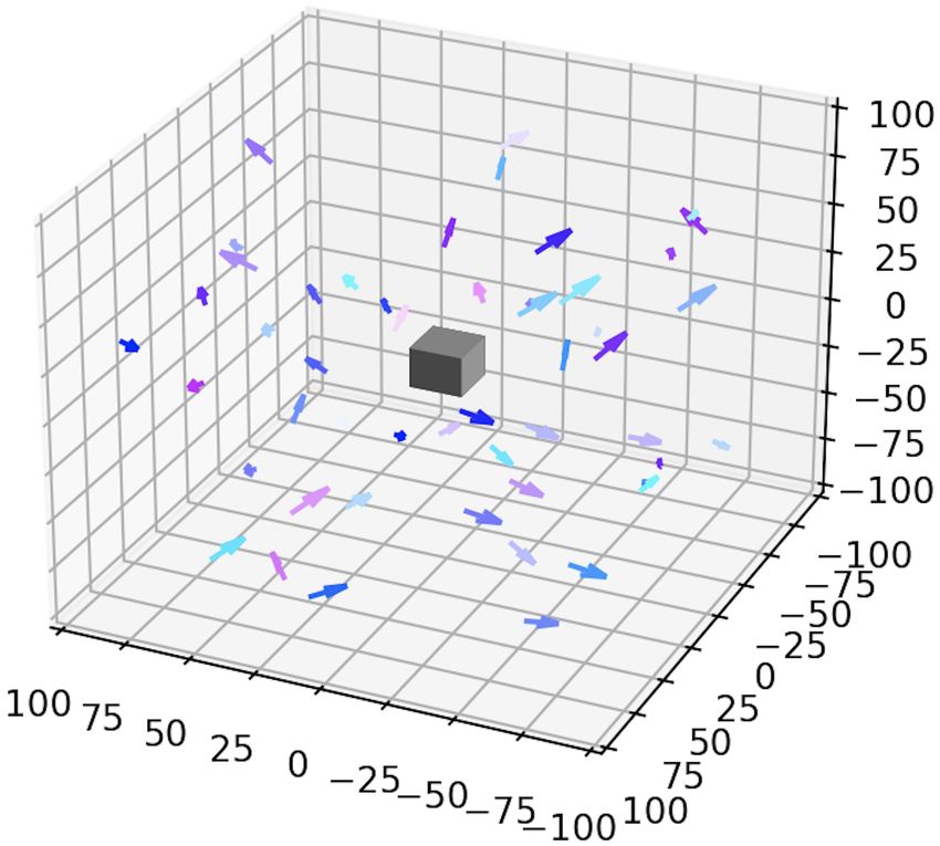
for each i = 1, . . . , j. To have access to µ̄j , we keep in mem-   much an agent can gain by replacing its policy π with a
ory every model µj , j ∈ {1, . . . , J} and, in order to sam-        best response π 0 , when the rest of the population plays π:
ple points according to µ̄j for a fixed j, we sample points          φ(π) := max 0
                                                                                   J(µ0 , π 0 , µπ ) − J(µ0 , π, µπ ). If φ(π̄j ) → 0
                                                                                  π
from µi , i ∈ {1, . . . , j}, with probability 1/j. These points     as j increases, FP approaches a Nash equilibrium. To cope
are then used to learn the distribution µ̄j with an NF, as it is     with these issues, we introduce the following ways to mea-
needed both for the reward and to sample the starting state of       sure progress of the algorithm:
an agent during the process of learning a best response policy.
                                                                        • Performance matrix: we build the matrix M of per-
4   Experiments                                                           formance of learned policies versus estimated distri-
                                                                          butions. The entry Mi,j on the i-th row and the j-
Environment. We implemented the environment as a cus-                     th column ish the total γ-discounted sum of rewards:
tom OpenAI gym environment to benefit from the power-                                   PT                                              i
                                                                                                 t
                                                                          Mi,j = E         t=0 γ   rt,i | s0 ∼ µ̄i−1 , u t ∼ π j (.|st )  ,
ful gym framework and use the algorithms available in sta-
ble baselines [Hill et al., 2018]. We define a state s ∈ S                 where rt,i = r(st , ut , µ̄i−1 ), obtained with πj against
as s = (x, v) where x and v are respectively the vectors                   µ̄i−1 . The diagonal term Mj,j corresponds to the value
of positions and velocities. Each coordinate xi of the posi-               of the best response computed at iteration j.
tion can take any continuous value in the d-dimensional box             • Approximate exploitability: We do not have access to
xi ∈ [−100, +100], while the velocities are also continuous                the exact best response due to the model-free approach
and clipped vi ∈ [−1, 1]. The state space for the positions is a           and the continuous spaces. However, we can approxi-
torus, meaning that an agent reaching the box limit reappears              mate the first term of φ(π̄) directly in the Flock’n RL al-
at the other side of the box. We chose this setting to allow the           gorithm with SAC. The second term, J(µ0 , π̄, µπ̄ ), can
agents to perfectly align their velocities (except for the effect          be approximated by replacing π̄ with the average over
of the noise), as we look for a stationary solution.                       past policies, i.e., the policy sampled uniformly from the
   At the beginning of each iteration j of Fictitious Play, we             set {π0 , . . . , πj }. At step j, the approximate exploitabil-
initialize a new gym environment with the current mean dis-                                            1
                                                                                                            Pj−1
                                                                           ity is ej = Mj,j − j−1              k=1 Mj,k . To smoothen the
tribution µ̄j , in order to compute the best response.
   Model - Normalizing Flows. To model distributions, we                   exploitability, we take the best response over the last 5
use Neural Spline Flows (NSF) with a coupling layer [Durkan                policies and use a moving average over 10 points. Please
et al., 2019]. More details about how coupling layers and                  note that only relative values are important as it depends
NSF work can be found in the appendix.                                     on the scale of the reward.
   Model - SAC. To compute the best response at                      A 4-Dimensional Example. We illustrate in a four dimen-
each Flock’n RL iteration, we use Soft Actor Critic                  sional setting (i.e. two-dimensional positions and velocities)
(SAC) [Haarnoja et al., 2018] (but other PG algorithms would         how the agents learn to adopt similar velocities by controlling
work). SAC is an off-policy algorithm which, as mentioned            their acceleration. We focus on the role of β in the flocking
above, uses the key idea of regularization: instead of con-          effect. We consider noise it ∼ N (0, ∆t) and the following
sidering the objective to simply be the sum of rewards, an                              flock,i
                                                                     reward: rti = fβ,t          − kuit k22 + kvti k∞ − min{kxi2,t ± 50k},
entropy term is added to encourage sufficient randomization                    i
                                                                     where x2,t stands for the second coordinate of the i-th agent’s
of the policy and thus address the exploration-exploitation          position at time t. The last term attracts the agents’ positions
trade-off. To be specific, in our setting, given a popula-           towards one of two lines corresponding to the second coordi-
tion distribution
           hP       µ, the objective is to maximize:i Jµ (π) =       nate of x being either −50 or +50. We added a term regard-
              +∞ t
E(st ,ut )    t=0 γ r(xt , vt , ut , µt ) + δH(π(·|st )) , where H   ing the norm of the velocity to prevent agents from stopping.
denotes the entropy and δ ≥ 0 is a weight.                           Here we take kvti k∞ = max{|v1,t        i       i
                                                                                                                |, |v2,t |}. Hence, a possible
   To implement the optimization, the SAC algorithm follows          equilibrium is with two groups of agents, one for each line.
                                                                                                    flock,i
the philosophy of actor-critic by training parameterized Q-          When β = 0, the term fβ,t              encourages agent i to have the
function and policy. To help convergence, the authors of SAC         same velocity vector as the rest of the whole population. At
also train a parameterized value function V . In practice, the       equilibrium, the agents in the two groups should thus move in
three functions are often approximated by neural networks.           the same direction (to the left or to the right, in order to stay
   In comparison to other successful methods such as Trust           on the two lines of x’s). On the other hand, when β > 0 is
Region Policy Optimization (TRPO) [Schulman et al., 2015]            large enough (e.g. β = 100), agent i gives more importance
or Asynchronous Actor-Critic Agents (A3C), SAC is ex-                to its neighbors when choosing its control and it tries to have
pected to be more efficient in terms of number of samples re-        a velocity similar to the agents that are position-wise close to.
quired to learn the policy thanks to the use of a replay buffer      This allows the emergence of two groups moving in different
in the spirit of methods such as Deep Deterministic Policy           directions: one group moves towards the left (overall negative
Gradient (DDPG) [Lillicrap et al., 2016].                            velocity) and the other group moves towards the right (overall
   Metrics. An issue with studying our flocking model is             positive velocity).
the absence of a gold standard. Especially, we can not com-             This is confirmed by Fig. 1. In the experiment, we set the
pute the exact exploitability [Perrin et al., 2020] of a pol-        initial velocities perpendicular to the desired ones to illustrate
icy against a given distribution since we can not compute            the robustness of the algorithm. We observe that the approxi-
the exact best response. The exploitability measures how             mate exploitability globally decreases. In the case β = 0, we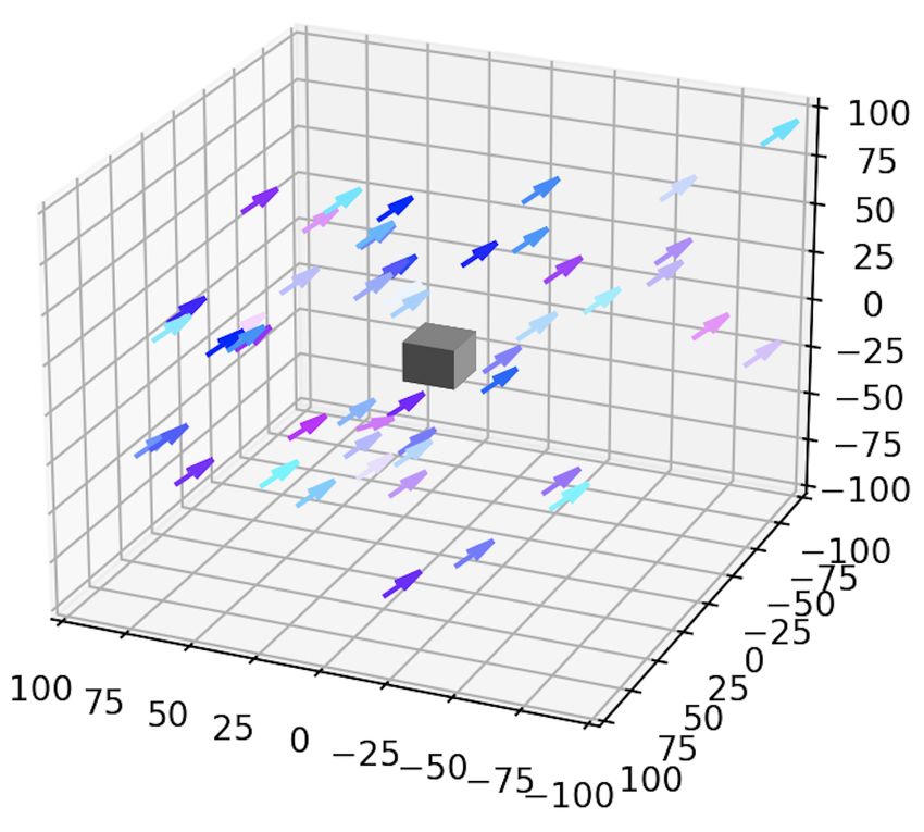
(a) Initial positions and velocities (b) At convergence
(a) Initial positions and velocities
0 (b) At convergence
12
80 0
20
10 50 20.0
60 20
Mean distribution
40 8 0 17.5
50 15.0
Mean distribution
60 40 6 40
100 12.5
4 150 10.0
80 20 60
200 7.5
2
100 0 0 10 20 30 40 50 60 70 80
80 250 5.0
0 20 40 60 80 100
Approximate Best Response
300 0 20 40 60 80
(d) Approximate exploitability 0 20 40 60 80
Approximate Best Response
(c) Performance matrix
(d) Approximate exploitability
(c) Performance matrix
Figure 1: Multi-group flocking with noise and β = 100.
Figure 2: Flocking with noise and many obstacles.
experimentally verified that there is always a global consen-
sus, i.e., only one line or two lines but moving in the same agents is large [Perolat et al., 2018]. [Guo et al., 2019] com-
direction. bined a fixed-point method with Q-learning, but the conver-
gence is ensured only under very restrictive Lipschitz condi-
Scaling to 6 Dimensions and non-smooth topology. We
tions and the method can be applied efficiently only to finite-
now present an example with arbitrary obstacles (and thus
state models. [Subramanian and Mahajan, 2019] solve MFG
non-smooth topology) in dimension 6 (position and velocity
using a gradient-type approach. The idea of using FP in
in dimension 3) which would be very hard to address with
MFGs has been introduced in [Cardaliaguet and Hadikhan-
classical numerical methods. In this setting, we have multi-
loo, 2017], assuming the agent can compute perfectly the best
ple columns that the agents are trying to avoid. The reward
flock,i response. [Elie et al., 2020; Perrin et al., 2020] combined FP
has the following form: rti = fβ,t − kuit k22 + kvti k∞ − with RL methods. However, the numerical techniques used
min{kxi2,t k} − c ∗ 1obs , If an agent hits an obstacle, it gets therein do not scale to higher dimensions.
a negative reward and bounces on it like a snooker ball. Af-
ter a few iterations, the agents finally find their way through 6 Conclusion
the obstacles. This situation can model birds trying to fly in
a city with tall buildings. In our experiments, we noticed that In this work we introduced Flock’n RL, a new numerical
different random seeds lead to different solutions. This is not approach which allows solving MFGs with flocking effects
surprising as there are a lot of paths that the agents can take to where the agents reach a consensus in a decentralized fash-
avoid the obstacles and still maximizing the reward function. ion. Flock’n RL combines Fictitious Play with deep neural
The exploitability decreases quicker than in the previous ex- networks and reinforcement learning techniques (normaliz-
periment. We believe that this is because agents find a way ing flows and soft actor-critic). We illustrated the method on
through the obstacles in the first iterations. challenging examples, for which no solution was previously
known. In the absence of existing benchmark, we demon-
strated the success of the method using a new kind of ap-
5 Related Work proximate exploitability. Thanks to the efficient represen-
Numerical methods for flocking models. Most work using tation of the distribution and to the model-free computation
flocking models focus on the dynamical aspect without op- of a best response, the techniques developed here could be
timization. To the best of our knowledge, the only existing used to solve other acceleration controlled MFGs [Achdou et
numerical approach to tackle a MFG with flocking effects is al., 2020] or, more generally, other high-dimensional MFGs.
in [Carmona and Delarue, 2018, Section 4.7.3], but it is re- Last, the flexibility of RL, which does not require a perfect
stricted to a very special and simpler type of rewards. knowledge of the model, allow us to tackle MFGs with com-
Learning in MFGs. MFGs have attracted a surge of inter- plex topologies (such as boundary conditions or obstacles),
est in the RL community as a possible way to remediate the which is a difficult problem for traditional methods based on
scalability issues encountered in MARL when the number of partial differential equations.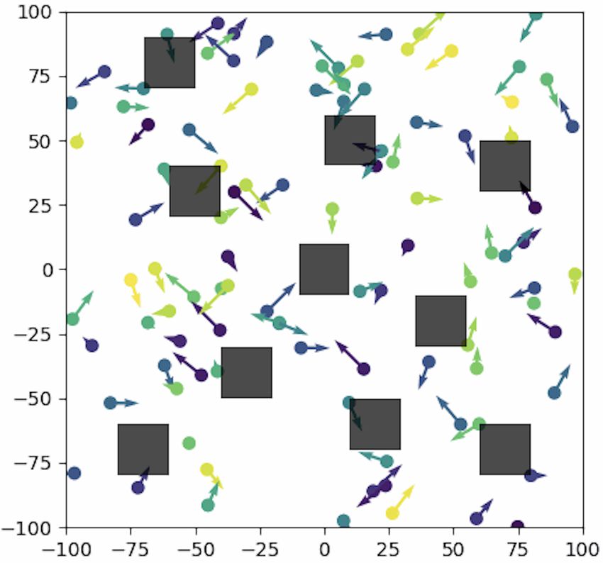
References                                                      [Lanctot et al., 2017] Marc Lanctot, Vinicius Zambaldi, Au-
[Achdou and Capuzzo-Dolcetta, 2010] Yves Achdou and                drunas Gruslys, Angeliki Lazaridou, Karl Tuyls, Julien
   Italo Capuzzo-Dolcetta. Mean field games: numerical             Perolat, David Silver, and Thore Graepel. A unified game-
   methods. SIAM J. Numer. Anal., 2010.                            theoretic approach to multiagent reinforcement learning.
                                                                   In proc. of NeurIPS, 2017.
[Achdou et al., 2020] Yves Achdou, Paola Mannucci, Clau-
   dio Marchi, and Nicoletta Tchou. Deterministic mean field    [Lasry and Lions, 2007] Jean-Michel Lasry and Pierre-
   games with control on the acceleration. NoDEA, 2020.            Louis Lions. Mean field games. Jpn. J. Math., 2007.
[Bailo et al., 2018] Rafael Bailo, Mattia Bongini, José A      [Lillicrap et al., 2016] Timothy P Lillicrap, Jonathan J Hunt,
   Carrillo, and Dante Kalise. Optimal consensus control of        Alexander Pritzel, Nicolas Heess, Tom Erez, Yuval Tassa,
   the Cucker-Smale model. IFAC, 2018.                             David Silver, and Daan Wierstra. Continuous control with
                                                                   deep reinforcement learning. In proc. of ICLR, 2016.
[Caponigro et al., 2013] Marco Caponigro, Massimo For-
   nasier, Benedetto Piccoli, and Emmanuel Trélat. Sparse      [Nourian et al., 2011] Mojtaba Nourian, Peter E Caines, and
   stabilization and optimal control of the Cucker-Smale           Roland P Malhamé. Mean field analysis of controlled
   model. Mathematical Control and Related Fields, 2013.           Cucker-Smale type flocking: Linear analysis and pertur-
                                                                   bation equations. IFAC, 2011.
[Cardaliaguet and Hadikhanloo, 2017] Pierre Cardaliaguet
   and Saeed Hadikhanloo. Learning in mean field games:         [Perolat et al., 2018] Julien Perolat, Bilal Piot, and Olivier
   the fictitious play. ESAIM Cont. Optim. Calc. Var., 2017.       Pietquin. Actor-critic fictitious play in simultaneous move
                                                                   multistage games. In Proc. of AISTATS, 2018.
[Carlini and Silva, 2014] Elisabetta Carlini and Francisco J.
   Silva. A fully discrete semi-Lagrangian scheme for a first   [Perrin et al., 2020] Sarah Perrin, Julien Pérolat, Mathieu
   order mean field game problem. SIAM J. Numer. Anal.,            Laurière, Matthieu Geist, Romuald Elie, and Olivier
   2014.                                                           Pietquin. Fictitious play for mean field games: Contin-
                                                                   uous time analysis and applications. In proc. of NeurIPS,
[Carmona and Delarue, 2018] René Carmona and François
                                                                   2020.
   Delarue. Probabilistic theory of mean field games with
   applications. I. 2018.                                       [Reynolds, 1987] Craig W Reynolds. Flocks, herds and
                                                                   schools: A distributed behavioral model. In Proc. of SIG-
[Carmona and Laurière, 2019] René Carmona and Mathieu
                                                                   GRAPH, 1987.
   Laurière. Convergence analysis of machine learning al-
   gorithms for the numerical solution of mean field control    [Rezende and Mohamed, 2015] Danilo Rezende and Shakir
   and games: II - the finite horizon case. 2019.                  Mohamed. Variational inference with normalizing flows.
                                                                   In proc. of ICML, 2015.
[Cucker and Smale, 2007] Felipe Cucker and Steve Smale.
   Emergent behavior in flocks. IEEE Transactions on au-        [Ruthotto et al., 2020] Lars Ruthotto, Stanley J Osher,
   tomatic control, 2007.                                          Wuchen Li, Levon Nurbekyan, and Samy Wu Fung. A
                                                                   machine learning framework for solving high-dimensional
[Durkan et al., 2019] Conor Durkan, Artur Bekasov, Iain
                                                                   mean field game and mean field control problems. PNAS,
   Murray, and George Papamakarios. Neural spline flows,           2020.
   2019.
                                                                [Schulman et al., 2015] John Schulman, Sergey Levine,
[Elie et al., 2020] Romuald Elie, Julien Perolat, Mathieu
                                                                   Philipp Moritz, Michael I. Jordan, and Pieter Abbeel. Trust
   Laurière, Matthieu Geist, and Olivier Pietquin. On the         region policy optimization. CoRR, abs/1502.05477, 2015.
   convergence of model free learning in mean field games.
   In proc. of AAAI, 2020.                                      [Shaw, 1975] E Shaw. Naturalist at large-fish in schools.
                                                                   Natural History, 1975.
[Guo et al., 2019] Xin Guo, Anran Hu, Renyuan Xu, and
   Junzi Zhang. Learning mean-field games. In proc. of          [Silver et al., 2018] David Silver, Thomas Hubert, Julian
   NeurIPS, 2019.                                                  Schrittwieser, Ioannis Antonoglou, Matthew Lai, Arthur
[Haarnoja et al., 2018] Tuomas Haarnoja, Aurick Zhou,              Guez, Marc Lanctot, Laurent Sifre, Dharshan Kumaran,
                                                                   Thore Graepel, Timothy Lillicrap, Karen Simonyan, and
   Pieter Abbeel, and Sergey Levine. Soft actor-critic:
                                                                   Demis Hassabis. A general reinforcement learning algo-
   Off-policy maximum entropy deep reinforcement learning
                                                                   rithm that masters chess, shogi, and Go through self-play.
   with a stochastic actor. CoRR, abs/1801.01290, 2018.
                                                                   Science, 2018.
[Hill et al., 2018] Ashley Hill, Antonin Raffin, Maximilian
                                                                [Subramanian and Mahajan, 2019] Jayakumar Subramanian
   Ernestus, Adam Gleave, Anssi Kanervisto, Rene Traore,
                                                                   and Aditya Mahajan. Reinforcement learning in stationary
   Prafulla Dhariwal, Christopher Hesse, Oleg Klimov, Alex
                                                                   mean-field games. In proc. of AAMAS, 2019.
   Nichol, Matthias Plappert, Alec Radford, John Schulman,
   Szymon Sidor, and Yuhuai Wu. Stable baselines. https:        [Sutton et al., 1999] R. S. Sutton, D. Mcallester, S. Singh,
   //github.com/hill-a/stable-baselines, 2018.                     and Y. Mansour. Policy gradient methods for reinforce-
[Kobyzev et al., 2020] Ivan Kobyzev, Simon Prince, and             ment learning with function approximation. In proc. of
                                                                   NeurIPS. MIT Press, 1999.
   Marcus Brubaker. Normalizing flows: An introduction and
   review of current methods. PAMI, 2020.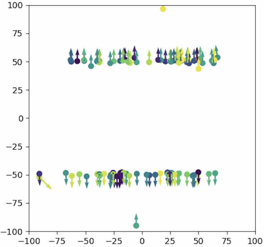
A     More numerical tests
A.1    A Simple Example in Four dimensions
We illustrate in a simple four dimensional setting (i.e. two-
dimensional positions and velocities hence the total dimen-
sion is 4) how the agents learn to adopt similar velocities by
controlling their acceleration.
   Here, we take it ≡ 0 (no noise), and we define the reward
as:
                       flock,i
                rti = fβ=0,t   − kuit k22 + kvti k22 .     (6)
We set β = 0 to have a intuitive example. The first term
encourages the agent to adapt its velocity to the crowd’s one,
giving equal importance to all the agents irrespective of their    (a) Initial positions and velocities                                                       (b) At convergence
distance. The second term penalizes a strong acceleration and
                                                                                        0
we added the last term (not present in the original flocking
                                                                                        5                                                      40
model) to reduce the number of Nash equilibria and prevent
the agent to converge to a degenerate solution which consists                          10
                                                                                                                                               30

                                                                   Mean distribution
in putting the whole crowd at a common position with a null                            15

velocity.                                                                              20                                                      20

   As the velocity is bounded by 1 in our experiments, there                           25
                                                                                                                                               10
are at least four obvious Nash equilibria in terms of velocity
                                                                                       30
that remain from reward (6): v̂ti ≡ (−1, −1), (−1, 1), (1, −1)                                                                                 0
                                                                                            0     5          10     15     20     25      30
and (1, 1), while the position is not important anymore and                                                Approximate Best Response

any distribution for the positions is valid. Experimentally,                                                                                         (d) Approximate exploitability
                                                                                                (c) Performance matrix
we observe that if we start from a normal initial distribution
v0i ∼ N (0, 1), then the equilibrium found by Flock’n RL is                                                 Figure 3: Flocking with an intuitive example
randomly one of the four previous velocities. However, if
we set the initial velocities with a positive or negative bias,
then we observe experimentally that the corresponding equi-
librium is reached. Thus, as we could expect, the Nash equi-
libria found by the algorithm depends on the initial distribu-
tion.
   In Fig. 3, we can see that the agents have adopted the same
velocities and the performance matrix indicates that the pol-
icy learned at each step of Flock’n RL tends to perform better
than previous policies. The exploitablity decreases quickly
because Flock’n RL algorithm learns during the first itera-
tions an approximation of a Nash equilibrium.
A.2    A Simple Example in Six Dimensions
We consider the simple example defined with reward from
Eq. (6) but now we add an additional dimension for the po-
sition and the velocity, making the problem six-dimensional.       (a) Initial positions and velocities                                                       (b) At convergence
As before, the agents are still encouraged to maximize their
                                                                                       0
velocities. We set β = 0 and we do not put any noise on
                                                                                                                                               250
the velocity dynamics. We can notice that experimentally a                             20                                                            50

consensus is reached by the agents as they learn to adopt the                                                                                  200
                                                                                                                                                     45
                                                                   Mean distribution

same velocities (Fig. 4b), even if the agents start from a ran-                        40
                                                                                                                                               150   40
dom distribution in terms of positions and velocities (Fig. 4a).                       60
                                                                                                                                               100
The performance matrix (Fig. 4c) highlights that the best re-                                                                                        35

sponse improves until iteration 40, which explains why there                           80                                                      50    30

is a bump in performance in the exploitability before the 40th                                                                                 0
                                                                                            0         20          40        60       80                   0     20    40    60     80
iteration.                                                                                                 Approximate Best Response
                                                                                                                                                     (d) Approximate exploitability
A.3    Examples with an obstacle                                                                (c) Performance matrix
We present an example with a single obstacle and noise in the                               Figure 4: Flocking for a simple example in dimension 6.
dynamics, both in dimension 4 and 6. In dimension 4, the
obstacle is a square located at the middle of the environment,
whereas in dimension 6 it is a cube. In dimension 4, we can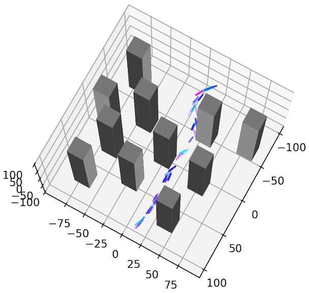
see in Fig. 5 that the agents that are initially spawned in the
environment with random positions and velocities manage to
learn to adopt the same velocities while avoiding the obstacle
(Fig. 5b). The same behavior is observed in dimension 6.
We also notice that the exploitability is slower to decrease in
dimension 6, similarly to what we observed with the simple
example without the obstacle.
(a) Initial positions and velocities (b) At convergence
0
250
20 80
(a) Initial positions and velocities (b) At convergence 200
Mean distribution
40 75
0 150
175
70
50 60
20 150 100
45 65
125 80 50
40
Mean distribution
100 40
60
0 0 10 20 30 40 50 60 70 80
60 0 20 40 60 80
75 35 Approximate Best Response
80 50 30 (d) Approximate exploitability
25
(c) Performance matrix
100 25
0 0 20 40 60 80 100
0 20 40 60 80
Approximate Best Response
100 Figure 6: Flocking in 6D with one obstacle.
(d) Approximate exploitability
(c) Performance matrix
Figure 5: Flocking in 4D with one obstacle.
A.4 Many obstacles in 4D
Finally, we present an example in 4D with many obstacles,
in the same fashion than the 6-dimensional example with the
columns located in the main part of the article.
B Normalizing Flows
In this section we provide some background on Normalizing
Flows, which are an important part of our approach.
Coupling layers A coupling layer applies a coupling trans-
(a) Initial positions and velocities (b) At convergence
form, which maps an input x to an output y by first split-
ting x into two parts x = [x1:d−1 , xd:D ], computing pa- 0
50
rameters θ = N N (x1:d−1 ) of an arbitrary neural network 50
20 0
(in our case a fully connected neural network with 8 hidden
50
Mean distribution
40
units), applying g to the last coordinates yi = gθi (xi ) where 40
100
i ∈ [d, . . . , D] and gθi is an invertible function parameterized 30
150
by θi . Finally, we set y1:d−1 = x1:d−1 . Coupling transforms 60
20 200
offer the benefit of having a tractable Jacobian determinant, 80 250
and they can be inverted exactly in a single pass. 10
300
0 10 20 30 40 50 60 70 80 0 20 40 60 80
Neural Spline Flows NSFs are based on monotonic Approximate Best Response
rational-quadratic splines. These splines are used to model (c) Performance matrix
(d) Approximate exploitability
the function gθi . A rational-quadratic function takes the form
of a quotient of two quadratic polynomials, and a spline uses Figure 7: Flocking in 4D with many obstacles.
K different rational-quadratic functions.
Following the implementation described in [Durkan et al.,
2019], we detail how a NSF is computed.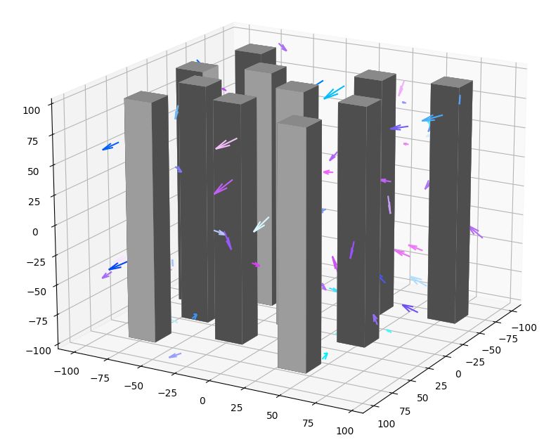
1. A neural network NN takes x1:d−1 as inputs and outputs
θi of length 3K − 1 for each i ∈ [1, . . . , D].
2. θi is partitioned as θi = [θiw , θih , θid ], of respective of
sizes K, K, and K − 1.
3. θiw and θih are passed through a softmax and multiplied
by 2B, the outputs are interpreted as the widths and
heights of the K bins. Cumulative sums of the K bin
K
widths and heights yields the K + 1 knots (xk , y k )k=0 .
4. θid is passed through a softplus function and is inter-
preted as the values of the derivatives of the internal
knots.
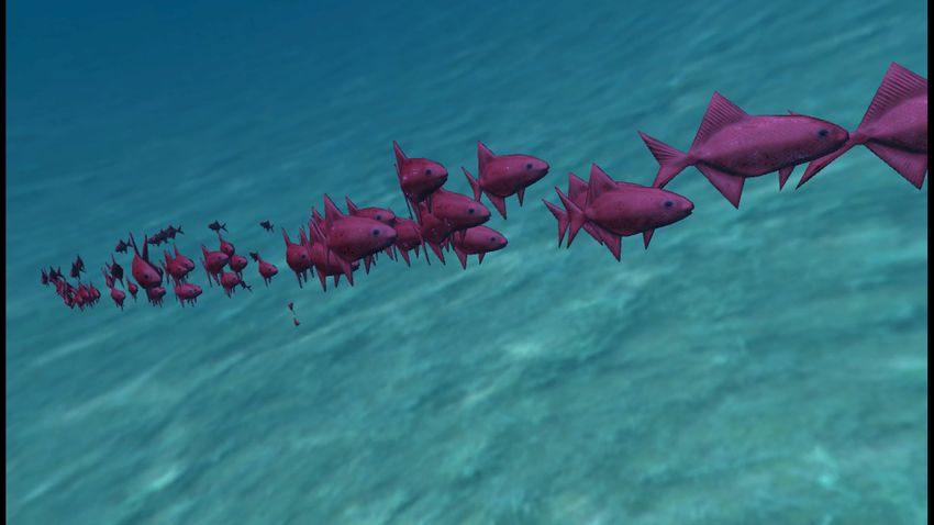
C Visual Rendering with Unity
Once we have trained the policy with the Flock’n RL algo-
rithm, we generate trajectories of many agents and stock them
in a csv file. We have coded an integration in Unity, making
it possible to load these trajectories and visualize the flock
in movement, interacting with its environment. We can then
easily load prefab models of fishes, birds, or any animal that
we want our agents to be. We can also load the obstacles and
assign them any texture we want. Examples of rendering are
available in Fig. 8.
Figure 8: Visual rendering with UnityYou can also read