THE RAYLEIGH-HARING-TAYFUN DISTRIBUTION OF WAVE HEIGHTS IN DEEP WATER - EARTHARXIV
←
→
Page content transcription
If your browser does not render page correctly, please read the page content below
The Rayleigh-Haring-Tayfun distribution of wave heights in deep water

                                                          S. Mendesa,b , A. Scottib
                                        Non-peer-reviewed preprint submitted to Applied Ocean Research

      a Group   of Applied Physics and Institute for Environmental Sciences, University of Geneva, Blvd. Carl-Vogt 66, Geneva, Switzerland
                    b Department of Marine Sciences, University of North Carolina at Chapel Hill, Chapel Hill, NC, 27599 USA

Abstract
Regarding wave statistics, nearly every known exceeding probability distribution applied to rogue waves has shown
disagreement with its peers. More often than not, models and experiments have shown a fair agreement with the
Rayleigh distribution whereas others show that the latter underpredicts extreme heights by almost one order of magni-
tude. Virtually all previous results seem to be microcosms, special cases of the underlying essence of this phenomenon.
The present work focuses on the apparent contradiction among the majority of previous works. Based on the issue
of strong uneven distribution of rogue waves found in Stansell (2004), a new exceeding probability distribution for
rogue waves and the analysis of their uneven occurrence is conceived. The proposed distribution is a geometrical
composition of the most popular models for wave records (Longuet-Higgins, 1952; Haring et al., 1976; Tayfun, 1980)
with additional algebraic structures. The suggested distribution also obeys empirical physical bounds obtained from
the analysis of nearly 350,000 waves from storms recorded in North sea and supports the qualitative likelihood of
appearance interpretation based on the symbiosis among three sea state parameters.
Keywords: Rogue Wave, Exceeding Probability Distribution, Composition Law, Water Wave, Storms, Nonlinearity,
Physical Bounds

1. Introduction

    The seminal work of Longuet-Higgins (1952) introduced a Rayleigh distribution (normal) of wave heights for
a narrow-banded sea, henceforth abbreviated as RD. The observation of the so-called Draupner wave in the mid
’90s brought a renewed interest on the subject of rogue waves (Haver and Andersen, 2000; Haver, 2004), whose
unusually large amplitude and steepness seem to appear out of nowhere (Akhmediev et al., 2009b). Naturally, one of
the most important considerations for marine safety of offshore operations and ship traffic is the recurrence interval
of extreme waves in a particular sea state, also known as the return period, i.e. the required number of waves for
each observed rogue wave. The accurate forecast of rogue waves return period is paramount because these waves
cause a lot of damage to the industry (Faukner, 2002; Cruz and Krausmann, 2008). Given the numerous examples of
the destructive power of rogues, marine safety is one of the main concerns and purposes of this study. As such, the
drive to obtain cutting-edge knowledge about oceanographic, mathematical and meteorological conditions for ship
and offshore standards has received increased focus and importance over the last decade. Therefore, the complete
understanding of all possible physical processes of generation, modeling of the exceeding probability as well as
the creation of an accurate warning system for diametrical sea states are essential for the design of both marine
installations and ships.
    Due to both randomness in the forcing mechanism and the nonlinear dynamics underlying the evolution of the
wave field, a description of the sea state is necessarily statistical in nature. The statistical approach leading to the
RD describes the sea surface as a superposition of wavelets with different frequencies and directional spreading. The
simplest configuration of this group of waves is the assumption of a uniform distribution of wave phases. Although

    Email addresses: saulo.dasilvamendes@unige.ch (S. Mendes), ascotti@unc.edu (A. Scotti)

Preprint submitted to Elsevier                                                                                                 January 16, 2021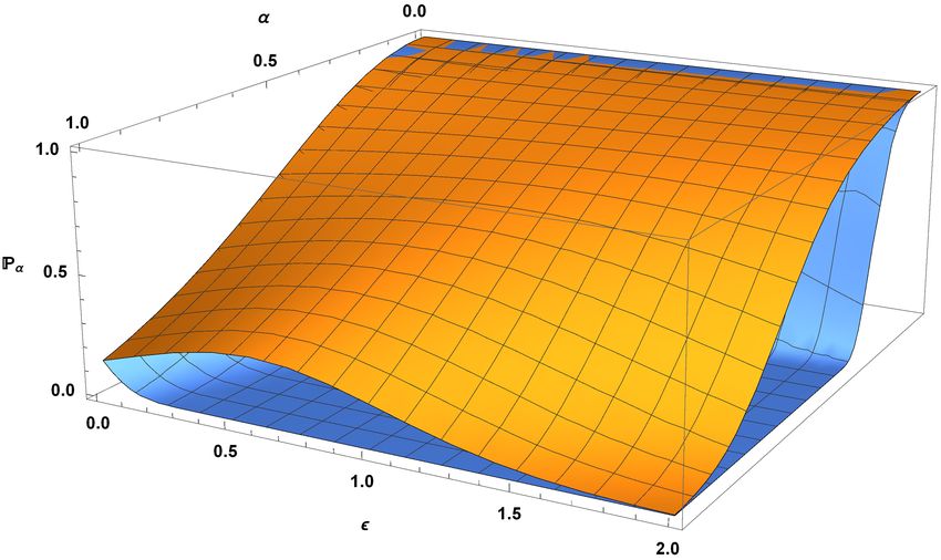
these approximate formulations have shown remarkable success in describing general ocean wave statistics and kine-
matics, some issues arise and is our interest to understand the deviation from these models that lead to the formation
of rogue waves in the upper tail of the distribution. For instance, based on RD, Øistein (2002) predicts that the famous
Draupner wave crest would appear only within a group of a million waves, almost two orders of magnitude higher
than the observed number of waves during the Draupner storm (Trulsen and Dysthe, 1997; Haver and Andersen, 2000;
Haver, 2004).
     Noticing the inaccuracy of the RD model prediction, strongly nonlinear mechanisms have been proposed to fill
the gaps in the standard model (Kharif and Pelinovsky, 2003; Dysthe et al., 2008; Onorato et al., 2013). Among
these nonlinear models, the so-called Nonlinear Schrödinger equations (NLSE) stand out as the most popular and
studied. They have been widely used to model rogue waves for the last three decades (Peregrine, 1983; Janssen,
2003), particularly in the context of unidimensional water wave fields (Akhmediev and Korneev, 1986; Akhmediev
et al., 2009a). NLS-type equations can be readily derived from the Euler equations if one assumes weak nonlinearity
(small steepness) and narrow-banded spectrum. A remarkable example of such derivation is the Zakharov equation
that assumes weak nonlinearity but deals with generalized bandwidth (Zakharov, 1968). Several other types of NLSE
have been studied, including the Dysthe and Davey-Stewartson equations (Davey and Stewartson, 1974; Dysthe,
1979). Nevertheless, the mathematical physics of the NLSE and related subjects have not yet been applied to the task
of prediction and warning system, but of rogue wave formation alone. However, this nonlinear mechanism has shown
limited success in explaining the formation of rogue waves. For instance, Fedele et al. (2016) explains that typical
oceanic wind seas features multidirectional wave fields which spreads the energy directionally thus diminishing the
effect of both modulational instability and/or nonlinear focusing, which are the established as the main mechanisms
of rogue wave formation. Moreover, the role of these instabilities in the formation of rogue waves appear of lesser
importance in finite depths. Secondly, theoretical analysis of third-order quasi-resonant interactions in Janssen (2003)
play a negligible role in rogue wave formation in realistic sea states (Fedele, 2015). Besides, these approximations
seem to lose importance when the steepness becomes large and their amplification by means of breathers are greatly
diminished. Nonetheless, these seemingly contradictory views could be unified (Dematteis et al., 2018, 2019).
     On the other hand (in a non-exhaustive bibliography), more down-to-earth models have been proposed in the mean-
time, with not less than a few dozen distributions have been proposed (Jahns and Wheeler, 1973; Haring et al., 1976;
Forristall, 1978; Tayfun, 1980, 1983; Ochi, 1986; Langley, 1987; Winterstein, 1988; Tayfun and Lo, 1989; Tayfun,
1990; Kriebel and Dawson, 1991; Ochi and Ahn, 1994; Winterstein et al., 1994; Cieslikiewicz, 1998; Kobayashi et al.,
1998; Srokosz, 1998; Forristall, 2000; Song et al., 2002; Prevosto and Bouffandeau, 2002; Krogstad and Barstow,
2004; Socquet-Juglard et al., 2005; Tayfun and Fedele, 2007). Most of these distributions include Stokes second-
order terms and the probability distribution is expressed in terms of the significant steepness and wave heights and
may include a depth parameter for shallow water waves (see Tayfun and Alkhalidi (2020) for a review on their
methodological differences). Additional methods have been applied such as Gram-Charlier expansions (Longuet-
Higgins, 1963; Al-Humoud et al., 2002; Mori and Yasuda, 2002) which highlights the importance of the skewness
and excess kurtosis of the surface elevation. Although an approach based on the Gram-Charlier covers water waves
of any bandwidth, it suffers from being computationally burdensome. In addition, this approach produces undesirable
negative probabilities and bounds for maximum and minimum surface elevations that are not compatible with the
physics of the system (Forristall, 2000).
     Despite the joint effort of several leading academic and private groups and in creating research projects to obtain
further understanding of this phenomenon, no consensus regarding the exceeding probability for rogue wave heights
or crests nor its generation mechanism has been reached (Bitner-Gregersen and Gramstad, 2015; Karmpadakis et al.,
2020). Furthermore, the lack of consensus inevitably leads to a hold on any intention to update offshore standards
by classification societies. Historically, the Agulhas current off of the southeast coast of South Africa has been the
first site where rogue waves could be easily identified (Mallory, 1974), nevertheless, specific sea state parameters
as well as other generation mechanisms implemented over that region did not reach success in predicting rogue
waves (Bitner-Gregersen and Gramstad, 2015). Likewise, the MaxWave project (Savina et al., 2003) proposed the
implementation of indices that coupled significant wave height and wave steepness as well as directional spreading as
a warning system for rogue waves in the weather forecasting. The suggested major index was mostly dependent on
the significant steepness (undefined in Savina et al. (2003)) and the significant wave height H1/3 , i.e. the mean wave
height among the 1/3 highest waves recorded in the time series. The two indices were implemented by Meteo France
and the occurrence of rogue waves was found to be weakly correlated with them. Numerous authors have attempted
                                                           2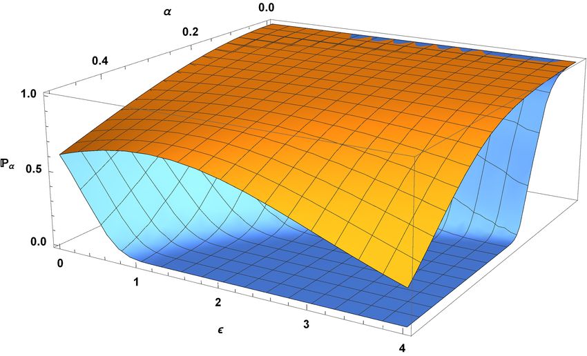
R                           R                                                       e
                                                                                                      H
                                                                             R                                            R
                                                                                                      e
                                                                                                      H
                               e
                               R                                                                                                           Te

                                                                                                                                  Te
            T                                                                    Te
                                                                        e
                                                                        R                                             e
                                                                                                                      R       e
                                                                                                                              R
                                                  e
                                                  H                                                               e
                                    R                               R                                             H
                                                                                              R                                                 R

                                                                                                              e
                                                                                                              H
        R                           R                                        R                                            R
                                                                                          R       R                                             e
                                                                                                                                                R
                                                                                      T
                                           e ◦H
                                        T ◦R  e                                  T                                                Te

                                                                                                                  H
                                                                                              R                                                 R
                           R                              R                                                       H

Figure 1: (Left) Graphic representation of the aimed composition rule as a three-dimensional f ◦ g and (Right) Possible compositions spanning all
paths over the cube edges.

to link spectral parameters and the occurrence of rogue waves with similar dire results, making the current state of
warning system not satisfactory (Bitner-Gregersen and Gramstad, 2015). Therefore, In this work we attempt to devise
an exceeding probability that explains the uneven spread of rogues among several storms as described by Stansell
(2004) and at the same time obey the physical limits obtained from the data (Mendes et al., 2021), whose dataset did
not include information on the directionality for the analysis, which can indeed affect the results obtained thereof.
The reader is referred to the most important references regarding experimental (Onorato et al., 2009; Waseda et al.,
2009; Toffoli et al., 2017) and numerical (Toffoli et al., 2008, 2009) analysis of the role of directionality and sea state
parameters affecting rogue wave statistics.

2. Rayleigh-Haring-Tayfun Model
    The analysis in Mendes et al. (2021), which is also indispensable to follow the notation in this study, has described
Stansell’s data in detail and highlighted the unevenness of the observed return period into further minutiae. We
advocate for the formulation of a distribution built through a geometrical composition that approaches the RD in the
appropriate limit. In view of the shortcomings of the distributions highlighted in chapter Mendes et al. (2021), we
will use a different strategy: we start with a narrow-band approximation of the geometrical composition followed by
the inclusion of nonlinear effects as a final step. Individually, the recovery of RD is achievable in limiting conditions
except for the Forristall (1978, 2000) models. Such constraint will be key to decide the final version of the sought
distribution. Regardless of the choice for the composition, equation (1) must recover the normal distribution. Let the
composition function be of the type (see figure 1):

                Pα = (Ji ◦ J j ) ◦ Jk ≡ Ji jk         ;       lim T (H > αH1/3 ) = Rα         ;       lim H(H > αH1/3 ) = Rα           .            (1)
                                                              ε→0                                     →0

With that in mind, we write a general expression for the distribution structure Ji jk ,
                         "                          2+δ̃ #
                              A p                                   ln Hα
              Ji jk = exp − 2+δ     1 + αH0 εθ − 1          , H0 = −        = 1 − 1.24 α + 1.09  2 α2 .                                           (2)
                            ε                                         2α 2

where H0 is the Haring root function. Then, we must find unique values for A, θ and δ̃ for a given δ that fulfills the
Rayleigh-Haring-Tayfun limit:
                                                       A · θ 2 α2  2 + δ̃        ε2θ−2−δ
                                       2+δ̃                              !
                  A p            θ
            lim 2+δ     1 + αH0 ε − 1        = 2α ∴
                                                 2
                                                                            lim               = 2α2 .              (3)
            →0 ε                                    4(2 + δ − θ) 2 + δ ε→0 (1 + αεθ )−3/2
                ε→0

Accordingly, we find θ = 1 + δ/2 the solution (A, δ, δ̃, θ) must be equal to (8, 0, 0, 1). In addition, Mendes et al. (2021)
introduced physical bounds for the variables α,  and ε, so that the following criteria should be fulfilled by established
                                                                         3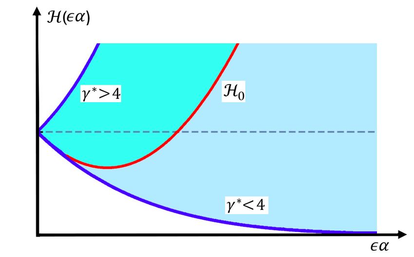
1.0
                                                                                                                ℛα
                                                                                                                ℋα (ϵ=0.2 ; γ=-1.5)

                                                     0.8                                                        ℋα (ϵ=0.2 ; γ=+1.5)
                                                                                                                ℋα (ϵ=0.4 ; γ=-2)

                             Exceeding Probability
                                                                                                                ℋα (ϵ=0.4 ; γ=+2)
                                                     0.6                                                        ℋα (ϵ=0.8 ; γ=-2)

                                                     0.4

                                                     0.2

                                                     0.0
                                                       0.0         0.5         1.0             1.5       2.0         2.5              3.0
                                                                                               α

                                                     Figure 2: Adjustment to Haring et al. (1976) by a factor γ as in eq. (8).

and forthcoming probability distributions:

                  Pα α > α∞ −→ 0 ; Pα ε > ε∞ −→ 0                                                        Pα α > kαk∞ −→ 0                 .

                                                                                                     ;                                          (4)

Following eq. (3), it is plain to find an expression for such an operation (see figure 1):
                                         r
                                             1                 e  = R(α) := e−2α2 .
                                    f :=
                                    e       − ln f     ∴ R R(α)                                                                                 (5)
                                             2

Hence, the composition law of RD with another function J(α) would produce,

                J ◦R         e  = J(α) ∴ lim T (α) ◦ H(α)
                    e ≡ J R(α)                               e    = lim H(α) ◦ T
                                                                               e (α) = R(α) .                                                   (6)
                        α                                                            →0                       →0
                                                                                     ε→0                       ε→0

Discarding cumbersome looking combinations and taking into account the constraint in eq. (3) as well as changing
the steepness from s to ε, the best version for eq. (2) is:
                                                  (    "q               #2 )
                                                 8
                               Pα = T R H(α) = exp − 2   1 + ε α H0 − 1      ,
                                                                  1/2
                                      e  e                                                                                                      (7)
                                                    ε

which we call the Rayleigh-Haring-Tayfun (RHT) model. It recovers Tayfun (1980) when  → 0, Haring et al. (1976)
when ε → 0 and Longuet-Higgins (1952) when both variables vanish, as intended. Since the negligible variability for
Haring et al. (1976) and Tayfun (1980) in response to sea states is well-known (Mendes et al., 2021), and in order to
preserve the Stokes expansion structure of Tung and Huang (1985), we modify the Haring function:
                        "                             #             (    "q               #2 )
                                                  2 2 γ                 8            γ/2

            Hα,γ   = exp − 2α 1 − 1.24 α + 1.09  α
                             2
                                                         ∴ Pα,γ = exp − 2   1 + ε α H0 − 1      ,                                               (8)
                                                                       ε

to obtain the Modified Rayleigh-Haring-Tayfun (MRHT) model. Figure 2 shows that eq. (8) is much more flexible
than Haring et al. (1976). However, the modified version of Haring et al. (1976) will violate the monotonicity of the
exceeding probability (Rohatgi, 1976) and corollaries (Mendes, 2021), thus, we shall attempt to find a remedy for
anomalies that may arise.

3. Tracking γ

    In order to assess the validity of eq. (7) regarding the parameter γ we need to find clues on how to express it in
terms of the given sea parameters in eq. (4). According to Figure 16 in Mendes et al. (2021), a combination of high
                                                                                           4
0 0
-2 -2
Longuet-Higgins Longuet-Higgins
-4 -4
log ℙ α
log ℙ α
ℙα (ϵ=1/5 ; ε=1/5 ; γ=-1) ℙα (ϵ=1/5 ; ε=1/5 ; γ=-1.0)
ℙα (ϵ=1/10 ; ε=1/10 ; γ=-1) ℙα (ϵ=1/10 ; ε=1/10 ; γ=-1.2)
-6 -6
ℙα (ϵ=1/20 ; ε=1/20 ; γ=-1) ℙα (ϵ=1/20 ; ε=1/20 ; γ=-1.4)
ℙα (ϵ=1/5 ; ε=1/5 ; γ=+1) ℙα (ϵ=1/5 ; ε=1/5 ; γ=+0.3)
-8 -8 ℙα (ϵ=1/10 ; ε=1/10 ; γ=+0.6)
ℙα (ϵ=1/10 ; ε=1/10 ; γ=+1)
ℙα (ϵ=1/20 ; ε=1/20 ; γ=+1) ℙα (ϵ=1/20 ; ε=1/20 ; γ=+1.2)
-10 -10
0.0 0.5 1.0 1.5 2.0 2.5 3.0 0.0 0.5 1.0 1.5 2.0 2.5 3.0
α α
Figure 3: The inspection of Figure 16 in Mendes et al. (2021) according to the MRHT model with (left) increasing absolute values of ( , ε) with
fixed γ in groups of fixed ratio ε/ and (right) a tentative change in γ to make each group have negligible variation.
0
Longuet-Higgins
ℙα (ϵ=1/5 ; ε=1/12)
-2
ℙα (ϵ=1/10 ; ε=1/15)
ℙα (ϵ=1/20 ; ε=1/20)
-4
log ℙ α
-6
-8
-10
0 1 2 3 4
α
Figure 4: (Left) Testing of Mendes et al.’s Figure 16 according to the MRHT model with increasing absolute values of ( , ε) and ratio ε/ with
fixed γ = −2 and (Right) Sketch of the function γ = γ(ℵ1 , ℵ2 ).
steepness and high height-to-depth ratio should lead to low probability. Likewise, a combination of low ε and low
should return the very same outcome. That is because at fixed nonlinearity η1/3 , according to Table 4 of Mendes et al.
(2021) we may use the approximation ln Pα ∼ ε/ for qualitative analysis. However, as expected, Figure 3 shows
this picture to not be too simplistic as described in the aforementioned table. We clearly see that when the probability
will give skewed behavior depending on the sign of γ, thus suggesting that if γ = γ(φ), with an unknown function of
sea parameters φ, given the central spot γ(φc ) := 0, we see that the γ function is skewed towards positive increments
of φc . Therefore, whatever γ may be, a large deviation from γ(φc ) will affect the exceeding probability significantly
with fixed (, ε). Now, according to Table 4 and Figure 11 of Mendes et al. (2021), the mediator when the latter
two parameters are fixed is the nonlinearity η1/3 , hence, γ = γ(φ(η1/3 )). For further validation of this hypothesis,
Figure 4 (left) confirms that when γ, and thus η1/3 , is fixed, the higher the ratio ε/ the higher the probability. At least
theoretically, the MRHT model prescribes the exact same solution as the graphical description of Mendes et al. (2021):
higher significant steepness and lower height-to-depth ratio increases the probability while the inverse decreases the
probability, which also means that for fixed η1/3 this produces a lower ℵ1 and by extension, lower ℵ2 . Thus, one can
show that the Ursell number depends on these two parameters (see parameter definitions in Mendes et al. (2021)):
6H1/3 hλ1/3 i2 6hi3 6η21/3 hλ1/3 i 6η21/3
Ur ≡ = · ℵ 1 ℵ2 ≡ hi · ℵ21 . (9)
31π2 D3 31π2 ε2 31π2 D 31π2
Then, at fixed ℵ1 , we conclude that the Ursell number will increase, thus, Figure 3 (right) has identical probabilities if
γ decreases when φ > φc or γ increases when φ < φc , suggesting a bell curve centered at φc . Moreover, for the same
52.0
ℋ0
cos-2 ( 0.8 ϵα ) e0.4 ϵα
1.5 cos2 ( 0.8 ϵα ) e-0.4 ϵα
Haring
1.0
0.5
0.0
0.0 0.5 1.0 1.5 2.0 2.5 3.0
ϵα
Figure 5: (Left) Sketch of Haring et al.’s root function and the necessary adjustments to the factor γ = γ∗ − 4 and (Right) tentative numerical
approximation for the sketch and H0 (α).
variation in we see that the region φ > φc has a much faster drop ∆γ ∼ −0.9 than its counterpart φ < φc increase
∆γ ∼ +0.4, producing a negative skewness. Nevertheless, the interval φ ∈ [φc , +∞) is of the order of its equivalent
λ2 /D ∈ [5, +∞), such that the seemingly slow decay in the region φ ∈ [0, φc ) is actually much faster because it covers
a very small interval λ2 /D ∈ [0, 5). Therefore, we may describe, asymptotically, the shape of γ(φ) as follows, depicted
in Figure 4 (right) and in agreement with Table 4 of Mendes et al. (2021):
γ φ ℵ(low)
1 , ℵ(low)
2 < γ φ ℵ(high)
1 , ℵ(high)
2 < γ φ ℵ(low)
1 , ℵ(high)
2 . (10)
Consequently, at fixed (, ε), the effort of the system to produce shallow water rogue waves should be in general, but
not always, much higher than for upper deep waters. Moreover, one may convince oneself that we need a translation
for the nonlinear measure γ∗ −→ γ + k in order to maintain a Gaussian shape (where k is some real non-negative
number), due to the fact that γ is typically negative and barely crosses to the positive realm. A quick back-of-the-
envelope reverse calculation using eq. (7) and the entries of Tables 1 and 3 of Mendes et al. (2021) will show that the
interval of interest here is −2 < γ < 1/2, hence, k = 4 is advised to obtain a mathematical expression as simple as
possible.
4. Modified Haring Function and a Constrained MRHT Model
Since we understand the rough shape of γ, we can apply the monotonicity condition to eq. (8), i.e. guaranteeing
that the derivative of the exceeding probability is non-positive, which is reduced to:
γ/2
αγ dH0
"
8H
#
d 1
ln Nα = 0
+ >0 .
1 − 1 (11)
ε
q
dα 2H0 dα
γ/2
1 + εαH0
Considering that the Haring function is strictly non-negative (see eq. (2)), we require:
αγ dH0 α dH0 2
1+ >0 ∴ >− , ∀ γ ∈ R∗ . (12)
2H0 dα H0 dα γ
We should, however, be even more careful, and seek the conditions below:
dH0 dH0
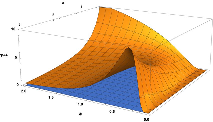
>0 ⇔ γ>0 ;Figure 6: 3D plot of the old (yellow) and the new version of Haring et al.’s distribution through eq. (14). Notice that Haring et al. (1976) violates
the depth-limited wave breaking section 4 of Mendes et al. (2021) by assigning a probability of 65.4% of finding wave heights H1/3 > 2D for any
dimensionless height α > 1/2. The new model (blue) estimates the probability for the same scenario to be of the order of 10−46 . In this plot we
used γ ≈ −4 for very deep water waves, in accordance with figure 4. Likewise, on the right, the old version predicts an exceeding probability of
nearly 20% of waves taller than H1/3 with H1/3 > D whilst the new model assigns a probability of 10−183 .
γ is not too negative, it can never satisfy the more strict condition of eq. (13). Therefore, instead of constraining
the strength of the ”meandering”, we rather reformulate the Haring function to obey eq. (13). Hence, our task is
to obtain a Taylor series capable of approximating the Haring function for α < 0.5 and departing from it to both
vanishing (γ < 0) and divergent (γ > 0) regimes in Figure 5 (left). Clearly, the best option for a Taylor series obeying
such constraints are of trigonometric behavior coupled to an exponential. Furthermore, the product of cosine and
exponential functions feature an expansion (up to coefficients) of the type 1 − O(x) + O(x2 ) + · · · , being optimal for
the modelling and generalization of eq. (2) and without undesirable trigonometric bouncing features. If, for the sake
of simplicity, we rewrite (8) with 2γ, we obtain
h √ i1/γ
H0 , γ = cos−2|γ| 0.8α e0.4α|γ| , ∀γ ∈ R , (14)
which is plotted in Figure 5 and matches the desired shape required by eq. (13). In addition, the new formulation
(14) does not assign finite exceeding probability for extreme values of α that would ultimately violate the bound,
as shown by Figure 6. Hence, possessing all the mechanisms necessary to repair (7), we rewrite the new exceeding
probability as: v 2
t
8 εα e 2|γ∗ −4|α/5
Pα (, ε, γ ) = exp
∗
+ .
− 1 − 1 (15)
√
ε
2
∗ −4|
−2|γ
4α/5
cos
Following the reasoning of the previous section, we start with the idea of γ∗ that is a function of ℵ1 and ℵ2 . For
instance, low intermediate water waves are approximately described by ℵ1 ℵ2 ≈ 40 Ur. Tentatively, one can easily
find a mathematical range for a good filter φ and thus fitting of the data, however, the filter should be obtainable from
the Ursell number at leading order. Then, if we reverse engineer the entries of Tables 1 and 3 of Mendes et al. (2021)
while combining eqs. (15) and (9), the most suitable clustering that makes the data a as homogeneous as possible
function γ(φ) is:
!3/5 5/7
121 φ−(68α/33) 0.305 7/4 7/4
γ∗ (α, φ) := , φ(ℵ1 , ℵ2 ) = 1 + ℵ1 1 + ℵ2 . (16)
η1/3
4
6α e1/φ − 1
Moreover, we introduce the error range for the calibration of γ∗ in order to get a closer fit to the expected values of
the latter that are not well covered by (16). Hence, we have:
!3/5 5/7
121 ± 3α φ−(68α/33)
γ (α, φ) ± ∆γ =
∗ ∗
. (17)
e1/φ − 1
6α
76
5.2-2.75ϕ 6
6.2-4ϕ
4.3 ϕ-2.5 (ⅇ1/ϕ -1)-1
5 4 ϕ-2.75 (ⅇ1/ϕ -1)-1
5
4
4
ℽ+4
3
ℽ+4
3
2
2
1 1
0 0
0.0 0.2 0.4 0.6 0.8 1.0 1.2 1.4
0.0 0.2 0.4 0.6 0.8 1.0 1.2 1.4
3(1+ℵ1 )7/4 (1+ℵ2 )7/4 / 10η41/3
3(1+ℵ1 )7/4 (1+ℵ2 )7/4 / 10η41/3
6 7
7.0-5.2ϕ 1.50 Ordn-waves
3.8 ϕ-2.89 (ⅇ1/ϕ -1)-1 6 1.75 sub-rogues
5
2.00 rogues
5 2.15 rogues
4
2.30 rogues
4 2.50 rogues
ℽ+4
ℽ+4
3
3
2
2
1 1
0 0
0.0 0.2 0.4 0.6 0.8 1.0 1.2 1.4 0.0 0.5 1.0 1.5 2.0
7/4 7/4 4
3(1+ℵ1 ) (1+ℵ2 ) / 10η 1/3 ϕ
Figure 7: Calibration of eq. (15) through the required γ (red dots) for reproducing Mendes et al.’s statistics with respective colors from (Bottom
Right) the model of γ∗ (α, ℵ1 , ℵ2 ) using eq. (16).
As a bonus, as shown in Figure 7, φ does such a good job at gathering homogeneously the γ extracted from Table 1 in
Mendes et al. (2021), that is also possible to find a generalized expression for γ∗ (α, ℵ1 , ℵ2 ) conveying a linear model.
However, our task is to provide a model that supports the interpretation of the underlying dynamics as suggested by
Table 4 of Mendes et al. (2021) and all the constraints and conditions thereof, in addition to the interpretations and
predictions of section 4 of Mendes et al. (2021). For instance, a linear γ model would make the distribution have a
maximum in large depths (or small wavelengths) deep water and be infinitely negative for shallow, thus making it
impossible to form rogue waves. Thence, for the reasons already pointed out by eq. (10) and in Figure 4, we select the
model of eq. (16), whose non-trivial shape is depicted in Figure 8 (left). Generally, as conveyed by previous versions
of Pα (7, 8, 15), an α approaching zero should obtain a 100% of exceeding probability as attested by Longuet-Higgins
(1952). Likewise, we need to find the limit of Pα in eq. (15) when γ∗ is very large. First, however, we remind the
reader that:
lim γ∗ · α ≈ O α2/5 = 0 . (18)
α→0
γ∗ →+∞
Ergo, applying (18) into (15), we readily conclude:
8 εα 2
) (
2
lim Pα (γ ) ≈ exp − 2
∗
≈ e−2α = 1 , (19)
α→0 ε 2
γ →+∞
∗
Thus being consistent with the standard limit of Rα when α approaches zero, proving another advantage of using the
modified Haring function of eq. (14) instead of eq. (2).
84
ℽ✶ - 4
(ℽ ✶ - 4) 1
3
2 α2
(ℽ ✶ - 4) e-α ∞
2 2 α2
2 (ℽ ✶ - 4) e-3 α ∞
ℽ⊕
1
0
-1
0 5 10 15
α
Figure 8: (Left) 3D plot of γ∗ function of eq. (16) with varying dimensionless heights (1/3 6 α 6 3) and the auxiliary parameter φ (ℵ1 , ℵ2 ) and
(Right) Damping of γ⊕ for the storm 172. The upper bound for the storm is α∞ = 4.72. The simpler modification quickly departs from eq. (16) for
mid-range α whereas the full modification reaches its peak before α∞ .
4.1. Smoothness near α∞
Nevertheless, we still need to obtain a bound for the specific case of very large dimensionless wave heights and
obey the monotonicity condition (Mendes, 2021). This bound is also related to the first part of condition (4). The main
issue at hand is that it is typically very complicated to satisfy the monotonicity and non-negative second derivative
(henceforth called ”meandering”) simultaneously. Often distributions obey one and not the other. Moreover, the
second derivative would look terribly complicated in eq. (13). Instead of finding a general formula for H0γ obeying
monotonicity and ”meandering” at once, it seems more realistic to stick to the general solution for monotonicity and
modify it with a truncation that makes the ”meandering” arise for selected storms. In other words, it might be too
complicated to find a ”meandering” formula for all storms, and even doing so, this expression would not affect the
less complex form of eq. (24). Lastly, we notice that the meandering for small negative values of γ starts about or
after its bound α∞ (Mendes, 2021), whereas when feasible, the ”meandering” should happen in the vicinity but not
after its upper normalized height bound. Accordingly, when the normalized height approaches α∞ the corresponding
value of γ∗ must drop, because eq. (13) at a very large γ requires a very high slope for H0 capable of producing Planck
scale low probabilities (see Figure 6). However, this drop can not change the sign of γ, in order to not violate the
meandering condition, such that this modification should be as shown in Figure 8 (right). Notice that at α > α∞ will
reduce the distribution to the Tayfun (1980) form, however, at so large normalized heights it also produces Planck
scale low likelihoods as required by eq. (1). Noticeably, the same work could be obtained by making γ to flatten out
at α ∼ α∞ and then grow again at α > α∞ , producing likelihoods as low as in Figure 6, however, the modification for
γ would be even more burdensome. These considerations are important for super-rogue waves and the ”meandering”.
Using the four storms with highest rogue wave occurrence and eq. (4) as liaisons, we modify γ:
ξ2 α 2
α∞ /40 α2
γ⊕ tanh 6φ α∞
3 · exp −4 α∞
2
B1 := = , (20)
γ
h 2α
i
∞
tanh 2α+25α2 (ln ξ)3
∞
Where ξ denotes the bound availability, i.e. how the combined typical maximum normalized heights α? and kαk∞ /
measure up the upper bound α∞ . Therefore, we obtain,
!#1/2
λ2
r "
16 2πD
ξ := α∞ = α∞ hs s i · + 4 tanh . (21)
α? kαk∞ 7 D λ2
In Figure 8 (right) we show the differences between models (16) and (20): the first sharply increases in the vicinity
of α∞ whereas the second maintains a stable trajectory of small values for γ⊕ . From Figure 9 (right) the roles played
by each parameter becomes clear: ξ controls the strength of the meandering, φ controls the sign of γ and also affect
90
ℽ⊕ (α∞ = 5 ; ϕ = 4/3 ; ξ = 1.75)
4
ℽ⊕ (α∞ = 4 ; ϕ = 4/3 ; ξ = 1.75)
-2 ℽ⊕ (α∞ = 3 ; ϕ = 4/3 ; ξ = 1.75)
3
ℽ⊕ (α∞ = 3 ; ϕ = 2/5 ; ξ = 1.25)
ℽ⊕ (α∞ = 4 ; ϕ = 2/5 ; ξ = 1.25)
-4 2 ℽ⊕ (α∞ = 5 ; ϕ = 2/5 ; ξ = 1.25)
ℽ⊕ (α∞ = 3 ; ϕ = 4/3 ; ξ = 1.50)
log ℙα
ℽ⊕
Longuet-Higgins (1952)
-6 1
Storm 29
Storm 149
-8 0
Storm 90
Storm 172
Storm 132 -1
-10
Storm 28
Storm 146 -2
-12
0 1 2 3 4 5 6 0 2 4 6 8 10 12 14
α α
Figure 9: (Left) Probability model variability for the storms in Mendes et al. (2021) due to (φ, ξ) with modified γ⊕ = γB1 and B∞
2 = 2 and (Right)
deep and shallow water wave regimes using their characteristics φ and attached to upper bounds α∞ .
ξ strength (because shallow water waves with higher ξ still produced a smaller ∆γ than a deep water counterpart),
while an increasing α∞ diminishes the likelihood (if everything in eq. (15) is fixed except γ), as per condition (13) a
more positive γ is attached to a positive slope H0 producing very low probabilities and vice-versa, partially explaining
why the storms with highest (on average) bounds α∞ on Table 5 of Mendes et al. (2021) are those with the smallest
ratio kαk/α∞ . This interpretation is also roughly supported by our conjectures in sections 5.3.2 and 5.5 in Mendes
et al. (2021), as when α∞ increases due to an increase in hhδ2 ii, a decrease in Eα follows. Notably, the ”meandering”
strength due to ξ is also corroborated by Figure 9 (left): When φ ∼ φc , e.g. the peak of γ, a higher bound availability
will produce higher distributions until it finally creates the ”meandering”. However, the tipping point towards the
”meandering” will depend on (η1/3 , , ε) altogether. As expected, when ξ is smaller, the meandering does not happen,
with a further observation that variations in φ seem to be symmetrical both to γ⊕ and RD. Note, however, that Figure
9 (right) is a function of α and not φ as in Figure 4 (right). Lastly, is important to note that if B1 ∼ e−α /α∞ we
2 2
would produce very similar results, leading to the same conclusion that a smaller bound α∞ would produce a stronger
lowering of γ(α), and thus, producing a ”meandering” and possibly avoiding overthinking for any qualitative analysis.
On the other hand, the more complex function B1 (ξ) brings in richer interpretation, which validates its choice. A
further modification of interest, but not necessarily mandatory if we use B1 ∼ e−α /α∞ , is related to the exponent of
2 2
the trigonometric function that is a Taylor expansion of Haring et al. (1976) in eq. (15). The new exponent shall read
(see Figure 10, left): !
7α∞ 7α∞ h i−1
B2 := 2 + · tanh 1 + e(α∞ −α)/ξ . (22)
8αξ 8αξ
The main effect of B2 is to enhance the cosine exponent in the vicinity of the bound α∞ without affecting the bulk
waves significantly. Furthermore, very high bound availability is counter-productive towards B2 , thus creating a
balance between B1 and B2 contributions.
Overall, the uneven occurrence of rogue waves is mostly due to a strong variation in γ when variations in and ε
are small, such as in Mendes et al. (2021). This can be seen in 7 as the variations in γ to produce the same probability
narrows as α decreases. In this sense, in agreement with the interpretation of Mendes et al. (2021), a better rogue wave
definition would be one in which the storm parameters influence on γ grows considerably. Moreover, we observe a
tendency of higher rogue wave occurrence in deep and intermediate water waves for small η1/3 . In other words, it is
easier for γ to reach high non-negative values when φ < 1. Accordingly, typical shallow water waves with hi ≈ 1/5
tend to have high occurrence of rogue waves if the following holds:
!7/4 !7/4
3 30 1
1+ 1+ ∼1 ⇔ η1/3 ∼ 2.4 , (23)
10 η1/3
4 η1/3 5η1/3
thus, the ”meandering” in shallow water would require a herculean effort from the system to form rogue waves. On
other hand, through a proper combination of and ε is possible to form rogue waves in shallow water, though is
106
(α∞ = 5 ; ξ = 1.50) 1.4
(α∞ = 5 ; ξ = 1.75)
(α∞ = 10 ; ξ = 1.50) 1.2
5 (α∞ = 15 ; ξ = 1.50)
(α∞ = 15 ; ξ = 1.75) 1.0
ℙα / ℙα
0.8
4
2
0.6
Storm 29
3 0.4 Storm 90
Storm 172
0.2 Storm 132
Storm 146
2 0.0
0 1 2 3 4
0 10 20 30 40 50
α
α
Figure 10: (Left) Revisited function in eq. (15) with varying normalized height and bound availability and (Right) ratio of the distributions in
eqs. (15) and (24). For the majority of storms the simpler model is sufficient for an accurate analysis of rogue wave occurrence when 2 6 α 6 2.3.
0 -2.0
Longuet-Higgins (1952)
Storm 29
-2 -2.5 Storm 172
Storm 132
Storm 27
-4 -3.0
Storm 124
Storm 195
log ℙα
log ℙα
-6 -3.5
Longuet-Higgins (1952)
Storm 29
-8 -4.0
Storm 172
Storm 132
-10 Storm 27 -4.5
Storm 124
Storm 195
-12 -5.0
0 1 2 3 4 5 6 1.6 1.8 2.0 2.2 2.4 2.6
α α
Figure 11: Predicted uneven distribution among storms (Stansell, 2004) with Sub-Rayleigh and Super-Rayleigh regimes for both models in eq. (25).
unlikely to form as many rogue waves as in deep water. Therefore, the consequences arising from the present model
are in complete agreement with available in-situ data and numerical simulations (Glukhovskii, 1966; Bitner, 1980;
Chien et al., 2002; Didenkulova and Anderson, 2010; Didenkulova and Rodin, 2012; Barbariol et al., 2015).
5. Ultimate RHT Model
Combining the previous sections, the final version of the exceeding probability reads:
v 2
t
8 εα e 2|γ|αB1 /5
P̂α (η1/3 , , ε) = exp + ,
− 1 − 1 (24)
√
ε2
−|γ|B
4α/5
cos 2
Where γ, B1 and B2 are also functions of η1/3 , and ε, due to eqs. (16), (17), (20) and (22). Hence, the final picture
for the exceeding probability proposed is (Pα as in eq. (15))
P̂α ⇔ 1 − Pα /P̂α > 14 , α ∈ 2, +∞
Pα ⇔ 1 − Pα /P̂α 6 14 , α ∈ 2, +∞
P H > αH1/3 = .
(25)
P̂α ⇔ φξ > 43 α , α ∈ 1.5, 2
Pα ⇔ φξ < 3 α
, α ∈ 1.5, 2
4
11ID α > 1.75 α>2 α > 2.5 α>3
29 30 (31 ± 2) 12 (7.2 ± 0.5) 0 [0.5 ± 0.1] 0 [0.05 ± 0.02]
149 95 (100 ± 14) 26 (23.6 ± 1.8) 1 [1.6 ± 0.6] 0 [0.18 ± 0.09]
90 111 (103 ± 9) 20 (23.3 ± 1.2) 1 (1.1 ± 0.2) 0 [0.09 ± 0.03]
172 54 (49 ± 6) 9 (11.0 ± 0.8) 1 [1.0 ± 0.3] 1 [0.17 ± 0.14]
132 68 (81 ± 7) 14 (14.2 ± 2.2) 0 (0.3 ± 0.1) 0 [0.00 ± 0.00]
28 30 (47 ± 5) 6 ( 9.7 ± 0.5) 0 [0.2 ± 0.1] 0 [0.00 ± 0.00]
146 20 [17 ± 2] 4 ( 1.6 ± 0.2) 0 [0.0 ± 0.0] 0 [0.00 ± 0.00]
23 42 (32 ± 4) 5 ( 4.3 ± 0.9) 0 [0.1 ± 0.1] 0 [0.00 ± 0.00]
26 33 (47 ± 4) 4 ( 7.2 ± 0.1) 0 [0.1 ± 0.1] 0 [0.00 ± 0.00]
127 15 (14 ± 1) 2 ( 1.2 ± 0.2) 0 [0.0 ± 0.0] 0 [0.00 ± 0.00]
25 21 (26 ± 3) 2 ( 4.0 ± 0.9) 1 [0.1 ± 0.1] 0 [0.00 ± 0.00]
27 23 (25 ± 3) 1 ( 3.0 ± 0.6) 0 [0.0 ± 0.0] 0 [0.00 ± 0.00]
124 30 [20 ± 2] 0 ( 0.6 ± 0.2) 0 [0.0 ± 0.0] 0 [0.00 ± 0.00]
195 9 (7 ± 1) 0 ( 0.5 ± 0.1) 0 [0.0 ± 0.0] 0 [0.00 ± 0.00]
P
581 (590 ± 63) 105 (111.4 ± 11.1) 4 [5.0 ± 1.4] 1 [0.49 ± 0.26]
Rα 774 119 1 0
Table 1: Predicted values for the entries of Table 1 in Mendes et al. (2021) from our model Pα (15) inside round brackets and P̂α (24) with square
brackets. The proposed model clearly outperforms Longuet-Higgins’s distribution for a variety of normalized heights. Out of the 60 total entries
of this table, Longuet-Higgins’s distribution accurately predicts about 40% while the MRHT model accurately predicted 75% of them, whereas the
(15) model has nearly 70% of accuracy. Considering only the first two columns (with higher statistical significance), these accuracy percentages
are reduced to 25% and 70% respectively.
These conditions on the distribution choice seems to be a sort of phase transition. According to Figure 10, the models
Pα (15) and P̂α (24) are nearly indiscernible for the majority of storms in the interval 0 < α 6 2, and indeed
the model (15) is quite reliable when 1.50 < α < 2.25, showing very few exceptions to this rule. However, their
range of similarity is affected by sea parameter variations, as shown by the very same plot. Therefore, as Figure 11
shows, our final model matches these qualitative observations of uneven occurrence, variability (or stratification) of
the probability distribution as well as the super-rogue wave ”meandering”.
5.1. Overall Assessment
Most models focus on either explaining the geometry of the tallest wave in a storm (such as the Draupner wave)
or to predict accurate ocean wave statistics for fixed α = 2. Our model in eq. (25) intends to be a good mathematical
description for the entire interval α ∈ [1, α∞ ). As such, Table 1 shows the remarkable performance of eq. (25) across
four crucial fixed normalized heights, including Longuet-Higgins (1952) for the total count only (see Table 2 of
Mendes and Scotti (2020) for its individual performance). Contrary to Longuet-Higgins (1952), our model maintains
an error smaller than 20% in virtually all cases and smaller than 10% in half of all cases.
5.1.1. Super-rogue Wave Assessment
Despite several wave tank experiments and field observations published in the literature, most reports do not
mention a wave with a normalized height of α > 3 (hence called super-rogue waves), deserving special consideration.
The most studied individual rogue waves, the Draupner wave (Haver and Andersen, 2000; Øistein, 2002; Haver, 2004;
Walker et al., 2004; Adcock et al., 2011; Clauss and Klein, 2011; Adcock, 2017) and the Andrea Wave (Magnusson
and Donelan, 2013; Cherneva and Guedes Soares, 2014; Bitner-Gregersen et al., 2014; Donelan and Magnusson,
2017; Fedele et al., 2017) are well below this threshold. The characteristics of Stansell’s super-rogue wave are much
more remarkable than the famous Draupner and Andrea waves, as shown by Table 2. Applying the available data of
storm 172 found in Table 3 of Mendes et al. (2021) into (16), we obtain the storm average φ172 ≈ 0.523. According
to the conditions laid in eq. (25), we reevaluate the North Alwyn super-rogue wave minimum return period, obtaining
65,000 waves (6 days), equivalently a likelihood of 10−5 . As the storm 172 contains 23,591 waves (2 days and 4
hours), we obtain a maximum relative probability of 36% to find at least one super-rogue wave as reported by Stansell
12Observation H1/3 (m) λ1/3 (m) T z (s) H(m) H/H 1/3 Zc Zc /Zt Zc /H 1/3
Draupner 11.92 ≈ 326 11.20 25.01 2.098 18.49 2.84 1.55
Andrea 9.18 ≈ 212 9.02 21.14 2.303 14.97 2.43 1.63
Alwyn 5.64 ≈ 179 8.18 18.04 3.190 13.90 3.36 2.46
Table 2: Observations at depths of 130m, 130m and 70m (Magnusson and Donelan, 2013).
(2004). Notice, however, that using B1 ∼ e−α /α∞ would make this likelihood increase to 70-80% while not affecting
2 2
lower statistics (α < 2.5), being disfavored not on numerical grounds, but rather on the lack of physical interpretations
for this model.
On the other hand, more established distributions discussed in Mendes et al. (2021) would prescribe the respective
2
likelihoods for the North Alwyn super-rogue wave: e−2·(3.19) ∼ 10−9 (Longuet-Higgins, 1952), 4 · 10−8 (Haring et al.,
−12
1976), 3 · 10 (Forristall, 1978), 8 · 10 (Tayfun, 1980) and 3 · 10−8 (Forristall, 2000). Looking from another
−8
perspective, we can analyze the likelihood for the North Alwyn wave by models of rogue wave crest exceeding
2
probability. For instance, Longuet-Higgins’s crest model predicts a probability of e−8·(2.46) ∼ 10−21 for the North
Alwyn super-rogue wave crest. Considering the storm zero-crossing period of 8 s, the latter estimates a necessary
interval of 3 · 1014 years for this wave to appear at a fixed point in the ocean, or ten thousand times the age of
the universe. However, according to second-order models, the Draupner and Andrea wave crests should have an
exceeding probability of 5 · 10−7 (Øistein, 2002), 4 · 10−6 (Prevosto and Bouffandeau, 2002), 5 · 10−6 (Walker et al.,
2004), 6·10−7 (Forristall, 2005) and more recently 3·10−6 (Adcock, 2017), whereas Longuet-Higgins’s would estimate
2
e−8·(1.60) ∼ 10−9 . On the other hand, the best estimate for Draupner and Andrea (Adcock, 2017) would likely assign
an exceeding probability of 10−11 for the North Alwyn super-rogue wave height, the equivalent of 26,000 years.
6. Conclusions
Given the scope of this endeavor, a review of the results found in this paper are: the proposed exceeding probability
is the first in the literature to combine three major sea state variables that are readily available from hindcast and that
mathematically are implemented as three dimensionless variables (, ε, η1/3 ). Through a geometrically inspired model,
we have obtained much better predictions than the most prestigious distributions in the literature as discussed in
Mendes (2021). We have also implemented the relevant physical variables of ocean states of Mendes et al. (2021)
into our distribution. It is also the first to introduce a probability distribution attached to an interpretation based on a
the combination of these three dimensionless variables (as shown in figure 3 of Part I) while obeying all the bounds
on α, , ε. Moreover, it shows unique flexibility (oscillation around the Longuet-Higgins (1952), the ”equilibrium”
model) not found in any distribution from previous works. Additionally, our model prescribes an interpretation of
the combination of sea state parameters that could be a blueprint for rogue wave warning systems. Furthermore, it
does not depend heavily on skewness or kurtosis, which is the cause for turning Longuet-Higgins (1963) and similar
models into cumbersome and numerically impractical models.
Contrary to other models, the new exceeding probability is generous to higher rogue waves (α > 3) without
having any anomalous behavior for other α, such as Gaussian shape for the return period. The major innovation of
this work relies on the continuous approach to the exceeding probability distribution. In fact, we experimented the
same model for seven different values of the dimensionless wave height α and have conclusively shown how sea states
create variability in empirical distributions. Is important to note the remarkable accuracy of the presented model for
waves that are nearly rogues: it was expected that Longuet-Higgins’s model would be the best approximation for bulk
waves. Thought it wasn’t the original aim and scope of this work, improving the description of bulk waves by RD is
certainly welcome and of good value.
Forristall’s respected second model predicts that storm 124 has the highest probability of featuring rogue waves
(Mendes et al., 2021), as it has the highest steepness. In practice, this storm had no rogue wave and its return period
for sub-rogue waves is also higher than predicted by Longuet-Higgins (1952). On the other hand, Forristall (2000)
predicts a range of variability for the return period of all fourteen storms to be N ∈ [1046, 1500], more than two
times lower than Longuet-Higgins’s prediction, thus predicting 22 rogue waves for storm 124 alone. Accordingly,
13Forristall (2000) would foresee nearly 300 rogue waves appearing in the fourteen storms, almost three times the
number reported by Stansell (2004). Therefore, second-order models (theoretical, numerical and experimental) do not
produce uneven extreme wave distributions as observed in Stansell (2004). Moreover, additional distributions showed
no mathematical or numerical advantage in both fitting the rogue wave uneven occurrence and explaining the source
of this phenomenon, such as Naess (1985),Boccotti (1989),Tayfun (1990),Tayfun and Fedele (2007),Boccotti (2000)
(see Mendes et al. (2021) for a review).
Additionally, Barbariol et al. (2015) reports a study of metocean forcings on the maximum of the extreme wave
crests and demonstrated that depth-induced shoaling significantly decreased the maximum extreme wave crest, thus
implying that shallow water wave regime has lower probability of exceeding the rogue wave threshold, i.e. the shape
of γ. Moreover, it was also found that a current in opposition to wave train would increase the exceeding probability,
however, the increase in extreme wave crest was only of 4% with an opposing current with velocity of 0.4 m/s at the
surface. Comparing it to the Agulhas current that has a velocity of 2.1 m/s at the surface (Boebel et al., 2003), the
maximum increase of a extreme wave crest due to an opposing current would be of the order of 20%. Such an increase
is not enough to explain for example the North Alwyn super-rogue wave crest which is about 80% taller than expected
by Longuet-Higgins (1952).
Despite the remarkable success of both interpretative and predictive branches of the proposed model with physical
bounds laid down in Mendes et al. (2021), our model is vulnerable to large deviations from the average values of
η1/3 , and ε, as already expected in the storm geometry discussion from Mendes et al. (2021). We suggest that a group
of wave records should be combined and averaged-out and analyzed by eq. (15) if and only if the deviation of the
significant wave height and other major variables does not exceed 25%. Higher deviations will likely increase the
discrepancy between the prediction and observation of the return period of rogue waves and we believe that is the
most probable cause of disagreement among many studies, in particular the very large deviation among samples as
analyzed in Christou and Ewans (2014). Moreover, our model needs validation for upper intermediate and shallow
water waves, since the available data was obtained for an average λ2 ≈ 0.78D. Another future work will deal with
data having variations in water depth while maintaining the water wave regime. Finally, more data is needed for full
validation of the simpler and the complex RHT models presented, but regardless of its validity to other data sets it
represents a good toy model for explaining both underprediction and overprediction of the Longuet-Higgins’s model
and because its geometrical structure can be used for an ultimate generalization.
7. Acknowledgements
S.M. and A.S. were supported by the National Science Foundation under grant OCE-0729636.
References
Adcock, T., 2017. A note on the set-up under the draupner wave. J. Ocean Eng. Mar. Energy 3, 89–94.
Adcock, T., Taylor, P., Yan, S., Ma, Q., Janssen, P., 2011. Did the draupner wave occur in a crossing sea? Proc. R. Soc. A 467, 3004–3021.
Akhmediev, N., Ankiewicz, A., Soto-Crespo, J.M., 2009a. Rogue waves and rational solutions of the nonlinear schrödinger equation. Phys. Rev.
E 80, 026601.
Akhmediev, N., Ankiewicz, A., Taki, M., 2009b. Waves that appear from nowhere and disappear without a trace. Phys. Lett. A 373, 675–678.
Akhmediev, N., Korneev, V., 1986. Modulation instability and periodic solutions of the nonlinear schrödinger equation. Theor. Math. Phys. 69,
1089–1093.
Al-Humoud, J., Tayfun, M., Askar, H., 2002. Distribution of nonlinear wave crests. Ocean Eng. 29, 1929–1943.
Barbariol, F., Benetazzo, A., Carniel, S., Sclavo, M., 2015. Space-time wave extremes: The role of metocean forcings. J. Phys. Oceanogr. 45,
1897–1916.
Bitner, E.M., 1980. Non-linear effects of the statistical model of shallow-water wind waves. Applied Ocean Research 2, 63–73.
Bitner-Gregersen, E., Fernandez, L., Lefèvre, J., Monbaliu, J., Toffoli, A., 2014. The north sea andrea storm and numerical simulations. Natural
Hazards and Earth System Sciences 14, 1407–1415.
Bitner-Gregersen, E., Gramstad, O., 2015. Rogue waves: Impact on ships and offshore structures. DNV GL Strategic Research & Innovation
Position Paper .
Boccotti, P., 1989. On mechanics of irregular gravity waves. In: Atti della ASccad. naz. dei Lincei A386 19.
Boccotti, P., 2000. Wave mechanics for ocean engineering. Elsevier Oceanography Series .
Boebel, O., Rossby, T., Lutjeharms, J., Zenk, W., Barron, C., 2003. Path and variability of the agulhas return current. Deep-Sea Res. II 50, 35–56.
Cherneva, Z., Guedes Soares, C., 2014. Time-frequency analysis of the sea state with the andrea freak wave. Nat. Hazards Earth Syst. Sci. 14,
3143–3150.
Chien, H., Kao, C., Chuang, L., 2002. On the characteristics of observed coastal freak waves. Coastal Eng. 44, 301–319.
14Christou, M., Ewans, K., 2014. Field measurements of rogue water waves. J. Phys. Oceanogr. 9, 2317–2335.
Cieslikiewicz, W., 1998. Maximum-entropy probability distribution of wind wave free-surface elevation. Oceanologia 40, 205–229.
Clauss, G., Klein, M., 2011. The new year wave in a seakeeping basin: Generation, propagation, kinematics and dynamics. Ocean Eng. 38,
1624–1639.
Cruz, A., Krausmann, E., 2008. Damage to offshore oil and gas facilities following hurricanes katrina and rita: An overview. J. Loss Prev. Proc.
Ind. 21, 620 – 626.
Davey, A., Stewartson, K., 1974. On three-dimensional packets of surface waves. Proc. R. Soc. A 338, 101–110.
Dematteis, G., Grafke, T., Onorato, M., Vanden-Eijnden, E., 2019. Experimental evidence of hydrodynamic instantons: The universal route to
rogue waves. Phys. Rev. X 91.
Dematteis, G., Grafke, T., Vanden-Eijnden, E., 2018. Rogue waves and large deviations in deep sea. Proc. Natl. Acad. Sci. USA 115, 855–860.
Didenkulova, I., Anderson, C., 2010. Freak waves of different types in the coastal zone of the baltic sea. Nat. Hazards Earth Syst. Sci. 10,
2021–2029.
Didenkulova, I., Rodin, A., 2012. Statistics of shallow water rogue waves in baltic sea conditions: the case of tallinn bay. in: Proc. of the 2012
IEEE/OES Baltic Int. Symposium , 1–6.
Donelan, M., Magnusson, A.K., 2017. The making of the andrea wave and other rogues. Sci. Rep. 7, 44124.
Dysthe, K., 1979. Note on a modification to the nonlinear schrödinger equation for application to deep water waves. Proc. R. Soc. A 369, 105–114.
Dysthe, K., Krogstad, H., Muller, P., 2008. Oceanic rogue waves. Annu. Rev. Fluid. Mech. 40, 287–310.
Faukner, D., 2002. Shipping safety: A matter of concern. Ingenia, The Royal Academy of Engineering, Marine Matters , 13–20.
Fedele, F., 2015. On the kurtosis of deep-water gravity waves. J. Fluid Mech. 782, 25–36.
Fedele, F., Brennan, J., De Leon, S., Dudley, J., Dias, F., 2016. Real world ocean rogue waves explained without the modulational instability. Sci.
Rep. 6, 27715.
Fedele, F., Lugni, C., Chawla, A., 2017. The sinking of the el faro: Predicting real world rogue waves during hurricane joaquin. Sci. Rep. 7.
Forristall, G., 1978. On the distributions of wave heights in a storm. J. Geophys. Res. 83, 2353–2358.
Forristall, G., 2000. Wave crest distributions: observations and second order theory. J. Phys. Ocean. 30, 1931–1943.
Forristall, G., 2005. Understanding rogue waves - are new physics necessary? Proc. 14th Aha Huliko’a Winter Workshop .
Glukhovskii, B., 1966. Investigation of sea wind waves (in russian). Gidrometeoizdat Publisher .
Haring, R., Osborne, A., Spencer, L., 1976. Extreme wave parameters based on continental shelf storm wave records. Proc. 15th Int. Conf. on
Coastal Engineering, Honolulu, HI , 151–170.
Haver, S., 2004. A possible freak wave event measured at the draupner jacket january 1 1995. Proc. Rogue Waves 20-22 October IFREMER .
Haver, S., Andersen, O., 2000. Freak waves: Rare realizations of a typical population of typical realizations of a rare population? Proc. 10th Int.
Offshore Polar Eng. Conf. Seattle 3, 123–130.
Jahns, H., Wheeler, J., 1973. Long-term wave probabilities based on hindcasting of severe storms. J. Petrol. Technol. 25, 473–486.
Janssen, P., 2003. Nonlinear four-wave interactions and freak waves. J. Phys. Oceanogr. 33, 863–884.
Karmpadakis, I., Swan, C., Christou, M., 2020. Assessment of wave height distributions using an extensive field database. Coastal Eng. 157.
Kharif, C., Pelinovsky, E., 2003. Physical mechanisms of the rogue wave formation. Eur. J. Mech. B Fluids 22, 603–634.
Kobayashi, N., Herrman, M., Johnson, B., Orzech, M., 1998. Probability distribution of surface elevation in surf and swash zones. Journal of
Waterway, Port, Coastal and Ocean Engineering 124, 99–107.
Kriebel, U., Dawson, T., 1991. Nonlinear effects on wave groups in random seas. Journal of Offshore Mechanics and Arctic Engineering 113,
142–147.
Krogstad, H., Barstow, S., 2004. Analysis and applications of second-order models for maximum crest height. J. Offshore Mech. Arctic Eng. 126,
66–71.
Langley, R., 1987. A statistical analysis of non-linear random waves. Ocean Eng. 14, 389–407.
Longuet-Higgins, M., 1952. On the statistical distribution of the heights of sea waves. Journal of Marine Research 11, 245–265.
Longuet-Higgins, M., 1963. The effect of non-linearities on statistical distributions in the theory of sea waves. J. Fluid Mech. 17, 459–480.
Magnusson, A.K., Donelan, M., 2013. The andrea wave characteristics of a measured north sea rogue wave. J. Offshore Mech. Arctic Eng. 135,
031108.
Mallory, J., 1974. Abnormal waves in the south-east coast of south africa. Int. Hydrog. Rev. 51, 89–129.
Mendes, S., 2021. Towards the unification of rogue wave statistics i: On the necessary response of distributions to sea state variables. EarthArxiv .
Mendes, S., Scotti, A., 2020. Rogue wave statistics in (2+1) gaussian seas i: Narrow-banded distribution. Appl. Ocean Res. 99, 102043.
Mendes, S., Scotti, A., Stansell, P., 2021. On the physical constraints for the exceeding probability of rogue waves in deep water. EarthArxiv, to
appear in App. Ocean Res. .
Mori, N., Yasuda, T., 2002. A weakly non-gaussian model of wave height distribution random wave train. Ocean Eng. 29, 1219–1231.
Naess, A., 1985. On the distribution of crest to trough wave heights. Ocean Eng. 12, 221–234.
Ochi, M., 1986. Non-gaussian random processes in ocean engineering. Probabilistic Engineering Mechanics 1, 28–39.
Ochi, M., Ahn, K., 1994. Probability distribution applicable to non-gaussian random processes. Probabilistic Engineering Mechanics 9, 255–264.
Øistein, H., 2002. Statistics for the draupner january 1995 freak wave event. Proc. Int. Conf. on Offshore Mechanics and Arctic Eng. 2, 691–698.
Onorato, M., Cavaleri, L., Fouques, S., Gramstad, O., Janssen, P., Monbaliu, J., Osborne, A., Pakozdi, C., Serio, M., Stansberg, C., Toffoli, A.,
Trulsen, K., 2009. Statistical properties of mechanically generated surface gravity waves: A laboratory experiment in a three-dimensional wave
basin. J Fluid Mech. 627, 235–257.
Onorato, M., Residori, S., Bortolozzo, U., Montina, A., Arecchi, F., 2013. Rogue waves and their generating mechanisms in different physical
contexts. Phys. Rep. 528, 47–89.
Peregrine, D., 1983. Water waves, nonlinear schrödinger equations and their solutions. J. Aust. Math. Soc. Ser. B 25, 16–43.
Prevosto, M., Bouffandeau, B., 2002. Probability of occurrence of a ”giant” wave crest. Proc. Int. Conf. on Offshore Mechanics and Arctic Eng. 2,
483–490.
Rohatgi, V., 1976. An Introduction to Probability and Statistics. Wiley, New York.
15You can also read