Proposed approaches to systematic planning of research and monitoring to support a South African inland fisheries policy
←
→
Page content transcription
If your browser does not render page correctly, please read the page content below

Water SA 47(3) 367–379 / Jul 2021                                                                                                  Research paper
https://doi.org/10.17159/wsa/2021.v47.i3.11865

Proposed approaches to systematic planning of research and monitoring to support a
South African inland fisheries policy
S Hugo1*          and OLF Weyl1,2†
1
  DSI/NRF Research Chair in Inland Fisheries and Freshwater Ecology, South African Institute for Aquatic Biodiversity, Makhanda, 6140,
South Africa
2
  Department of Ichthyology and Fisheries Science, Rhodes University, Makhanda, 6140, South Africa
*
 Current affiliation: Department of Biological Sciences, Faculty of Science, Engineering and Agriculture, University of Venda,
University Road, Thohoyandou, 0950, South Africa
†
  Deceased

                                                                                                                      CORRESPONDENCE
    A South African inland fisheries policy will depend on a reliable long-term supply of social-ecological data      S Hugo
    covering freshwater fisheries at a broad geographic scale. Approaches to systematic planning of research
    and monitoring are demonstrated herein, based on a fishery-independent gillnet dataset covering 44 dams,          EMAIL
    and geographic information system maps of monthly and annual climate variables, human land use, and               sanet.hugo@univen.ac.za
    road access in a 5 km zone around 442 dams. Generalised linear mixed models were used to determine
    the covariates of gillnet catch per unit effort. Such covariates are required for a model-based process to        DATES
    select a subset of state-owned dams for a long-term fishery survey programme. The models indicated a              Received: 10 September 2020
    monthly climate influence on catch per unit effort and climatic drivers of fish species distributions. However,   Accepted: 14 July 2021
    unexplained variation is overwhelming and precludes a model-based survey design process. Non-hierarchical
                                                                                                                      KEYWORDS
    clustering of 442 dams was then done based on annual climate and human land use variables around dams.
                                                                                                                      classification analysis
    The resulting clusters of dams with shared climate and land use characteristics indicates the types of dams       fishery independent surveys
    that should be selected for monitoring to represent the full range of climate and land use characteristics.       freshwater fishery
    Surrounding land use could indicate the socioeconomic characteristics of fisheries, for example, dams that        geographic information system
    may support subsistence-based communities that require increased research effort. Finally, although primary       recreational fishing
    catchments could be useful for organising national-scale management, land use cover in the 5 km zone              small-scale fishing
    around dams varied widely within the respective primary catchments. Beyond these proposed approaches
    to plan research, this study also reveals various data deficiencies and recommends additional future studies      COPYRIGHT
    on other possible methods for systematic research planning.                                                       © The Author(s)
                                                                                                                      Published under a Creative
                                                                                                                      Commons Attribution 4.0
INTRODUCTION                                                                                                          International Licence
                                                                                                                      (CC BY 4.0)
South African freshwater impoundments play an important role in food security and poverty
alleviation, by housing fish populations that are valued for recreation and consumption (Ellender
et al., 2009; Beard et al., 2011; McCafferty et al., 2012; Beatty et al., 2017). Large-scale commercial
freshwater fisheries are generally economically unviable in South Africa (McCafferty et al., 2012;
Britz, 2015; Barkhuizen et al., 2016). However, recreational fishing has been well-established for
decades and contributes to local economies (Ellender et al., 2009; McCafferty et al., 2012; Britz,
2015). Small-scale and subsistence freshwater fisheries are widespread and increasing, but, due to
historical marginalisation and lack of institutional policy support, often conflict with recreational
fishers (Andrew et al., 2000; Hara and Backeberg, 2014; Britz, 2015; Tapela et al., 2015).
The need for an institutional policy for the sustainable management and equitable use of freshwater
fisheries has been discussed in a series of papers (e.g. Weyl et al., 2007; McCafferty et al., 2012; Hara
and Backeberg, 2014; Britz, 2015). These studies and others (e.g. Beard et al., 2011; Lynch et al.,
2016; Weyl et al., 2021) highlight the need for capacity building in the small-scale fishing sector
and preventing ecosystem degradation and overfishing that may be exacerbated by stakeholder
conflicts. Since 2016 the Department of Environment, Forestry and Fisheries of South Africa has
been developing the National Freshwater (Inland) Wild Capture Fisheries Policy following national
and international sustainable development guidelines and the ecosystem approach to fisheries (Beard
et al., 2011; Weyl et al., 2021). Policy development is supported by comprehensive social-ecological
data collated in two Water Research Commission scoping studies (Britz et al., 2015; Tapela et al.,
2015). Subsequently, in June 2018, the Southern African Society of Aquatic Scientists convened
a workshop to identify priority research questions and knowledge requirements for the policy
(Weyl et al., 2021).
Sustainable management in a national policy framework is dependent on data that can be readily
supplied with simple methods at a reasonable cost (Bonar and Hubert, 2002; Walmsley, 2002).
Currently the immediate knowledge requirements for policy development and implementation are
impeded by a lack of recent or long-term data on fishery stocks and socioeconomic characteristics
covering inland waterbodies across South Africa (McCafferty et al., 2012; Britz et al., 2015; Tapela
et al., 2015; Weyl et al., 2021). Like inland fisheries worldwide, South African dams’ ecological and
socioeconomic characteristics vary spatiotemporally, which precludes blanket management and

ISSN (online) 1816-7950                                                     367
Available on website https://www.watersa.net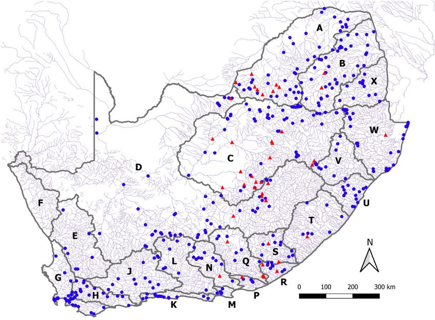
legislation and necessitates dam-specific adaptive management            gillnet dataset for determining useful relationships needs to be
and data collection (Hara and Backeberg, 2014; Britz et al.,             evaluated before a model-based survey can be designed.
2015; Weyl et al., 2021). Thus, comprehensive multi-disciplinary
                                                                         Given the current unavailability of a fishery monitoring
information is needed for each dam, including the population
                                                                         programme, a large-scale spatial analysis linking dams to
and life-history characteristics of the target species, types of users
                                                                         environmental variation and human activity indicators could
(e.g. recreational, subsistence or commercial), harvest methods
                                                                         identify dams with common social-ecological characteristics to
(e.g. gear type, intensity and frequency), and the economic
                                                                         prioritise for intensive multidisciplinary assessments (Beard et
and subsistence value (Weyl et al., 2007; Ellender et al., 2009;
McCafferty et al., 2012; Hara and Backeberg, 2014; Britz, 2015).         al., 2011; Camp et al., 2020). This approach is reminiscent of a
                                                                         conservation planning assessment, where high-biodiversity areas
Many rapid sampling methods can supply these data on a case-             that are threatened by human activities are revealed for priority
by-case basis (Beard et al., 2011; Tapela et al., 2015; Lorenzen         conservation actions under various cost and budget scenarios
et al., 2016). However, sustained long-term sampling is needed           (e.g. Rivers-Moore et al., 2011). Britz et al. (2015) used GIS climate
for adaptive management and to monitor effects from further              data and expert scores to identify river basins suitable for stocking
socioeconomic development and climate change (Dallas and                 with fishery species. However, there is a further need to quantify
Rivers-Moore, 2014; Paukert et al., 2017; Kao et al., 2020).             variation in human land use and climate, which may vary in their
Consequently, cost and labour input may need to be systematically        relative importance or have synergistic effects on fish populations
prioritised, focusing on fisheries that are most likely to be            (Dallas and Rivers-Moore, 2014; Camp et al., 2020; Jackson et
vulnerable to environmental stressors, generate reliable data,           al., 2020; Kao et al., 2020). An assessment of the characteristics
and support sustainable development goals (Beard et al., 2011;           of a large number of dams covering a large geographic area
Hara and Backeberg, 2014; Paukert et al., 2017). Lack of funding         complements both random stratified and model-based survey
and irregular data collection is pervasive on inland fisheries           design by evaluating the full range of variation in climatic and
worldwide, and overcoming the resultant data deficiencies is an          human-related covariates that need to be represented by selected
active area of research (Beard et al., 2011; Lorenzen et al., 2016;      sampling sites (Peel et al., 2012; Baker et al., 2019).
Lynch et al., 2016; Deines et al., 2017; Paukert et al., 2017). Some
tools suggested by recent global-scale studies (e.g. Lorenzen et al.,    Dams often support a combination of recreational and subsistence
                                                                         fishing (Britz et al., 2015; Ellender et al., 2009; Tapela et al.,
2016; Deines et al., 2017; Kao et al., 2020) may be useful in a South
                                                                         2015). Nevertheless, Weyl et al. (2007) suggest that common
African context, including using geographic information system
                                                                         characteristics like access, potential for tourism, and dominant
(GIS) climate and land use data, and using representative subsets
                                                                         fish species, predispose dams to different management types, e.g.,
of waterbodies for modelling general patterns.
                                                                         commercial, recreational, open access and community-managed
Fisheries-independent surveys (FIS) are widely regarded as               subsistence fishing. Dams located in an area with low economic
a valuable element of fisheries management, given that the               development (e.g., close to a rural town or subsistence farms)
sampling method can be standardised for comparison across                could be essential to local food security (Weyl et al., 2007; Britz
regions (Bonar and Hubert, 2002; McCafferty, 2012; Lorenzen              et al., 2015; Tapela et al., 2015). Dams located in remote, sparsely
et al., 2016). Although FIS can enable rapid stock assessment,           populated and untransformed areas, or in nature reserves with
such as assessing fish size distribution and community structure,        restricted access, may have a higher value as a recreational fishery
its real value lies in supplying catch per unit effort (CPUE) in a       (Weyl et al., 2007; Britz et al., 2015). Dams enclosed in commercial
long-term time-series to monitor how fish populations respond to         agricultural property may have limited scope in terms of fishery
changes in fishing pressure and the environment (Peel et al., 2012;      development (Weyl et al., 2007; Britz et al., 2015).
Lorenzen et al., 2016). McCafferty (2012) modelled CPUE of 26
                                                                         In the current study, the utility of existing data from fishery-
dams across South Africa based on a gillnet fleet with a matching
                                                                         independent gillnet surveys was examined in relation to
range of mesh sizes (see also Weyl et al., 2007; Winker, 2010).
                                                                         climatic and human-related factors, with the aim to provide the
This dataset, housed at the South African Institute for Aquatic
                                                                         background information needed to design a long-term model-
Biodiversity, has since expanded to 44 dams representing several
                                                                         based monitoring programme. Further, a broad range of dams
river basins and climate zones, and spanning the years 1998 to
                                                                         across South Africa is classified based on spatially associated
2017 (personal observation, see methods section). However, too
                                                                         climatic and human-related characteristics, to explore whether
few recurrent samples from individual dams are available for a
                                                                         such broad-scale classification could enable setting data collection
time-series.
                                                                         and management goals. Both these objectives focused on the local
To initiate a long-term monitoring programme, additions to the           area surrounding each dam following Ellender et al. (2009), who
gillnet dataset can focus on recurrent sampling of a representative      emphasized the local interactions between the Gariep Dam and
subset of dams across South Africa to produce reliable cost-             both subsistence and recreational fishers. However, dams likely
effective predictive estimates that can be extrapolated to               influence and are influenced by a larger surrounding region (e.g.
poorly sampled or unsampled dams (Lorenzen et al., 2016). A              a river drainage basin or primary catchment, Walmsley, 2002;
representative subset of dams can be selected through a model-           Jooste et al., 2014; Jackson et al., 2020). Therefore, the current
based survey design process, which has pertinent advantages              study also examined the available data in relation to South Africa’s
over a random stratified survey design process (Peel et al., 2012).      primary catchments, specifically whether land use characteristics
Model-based design accommodates multiple target species with             surrounding dams are comparable to general conditions in the
different habitat requirements, variable sampling effort due to          catchments and, consequently, whether catchments are useful
logistical and practical constraints (e.g. different dam sizes and       units within which to organise fishery management.
remote location of dams) and non-Gaussian response variables
(McCafferty, 2012; Peel et al., 2012). However, model-based survey       METHODS
design depends strongly on predictive covariates – a substantial
                                                                         Gillnet data
amount of initial data is required to determine the relationships
between CPUE and covariates and build the initial model (Peel            Between the years 1998 and 2017, 44 dams were sampled with
et al., 2012). McCafferty’s (2012) models did not reveal strong          a standard fleet of gillnets comprising five randomly positioned
covariate relationships, and therefore the utility of the expanded       panels, with stretched mesh sizes of 44 mm, 60 mm, 70 mm,

Water SA 47(3) 367–379 / Jul 2021                                                                                                         368
https://doi.org/10.17159/wsa/2021.v47.i3.11865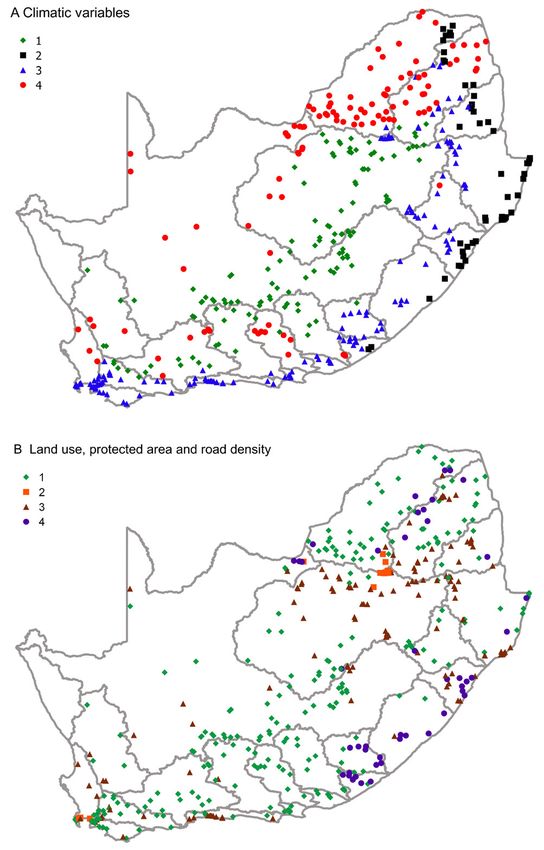
100 mm and 144 mm (9 m x 3 m panels, total size 45 m x 3 m),                temperature’) and annual precipitation for all 442 dams, as well as
and the data stored at the South African Institute for Aquatic              mean monthly temperature and precipitation matching the gillnet
Biodiversity. Dams were sampled within different years and                  monthly data (Hijmans et al., 2005). Land use variables included
months, many dams were sampled only once, and effort (number                percentage cover of commercial and subsistence cultivated area,
of nets deployed) varied among dams and months. Six species                 percentage formal urban build-up (cities and towns) and rural
that are most widespread in this dataset were examined: common              build-up (villages) and the percentage natural (untransformed)
carp (Cyprinus carpio, 31 dams), African sharp-toothed catfish              area (DEA, 2015). Protected area was a combination of formal
(Clarias gariepinus, 35 dams), Mozambique tilapia (Oreochromis              national parks, provincial reserves, and private game reserves
mossambicus, 14 dams), smallmouth yellowfish (Labeobarbus                   (SANParks, 2004).
aeneus, 21 dams), moggel (Labeo umbratus, 28 dams), and Orange
River mudfish (Labeo capensis, 21 dams). Catch per unit effort              Analyses
(CPUE) of all species summed was also examined and CPUE
                                                                            The relationship between monthly gillnet CPUE for each dam,
of all native cyprinids, i.e., the sum of L. aeneus, L. umbratus,
                                                                            and climatic variables, land use types, road density, protected
L. capensis, papermouth (Enteromius mattozi), largemouth
                                                                            area and dam area, was examined using generalised linear mixed
yellowfish (Labeobarbus kimberleyensis), largescale yellowfish
                                                                            effects models (R package ‘lme4’, Bates et al., 2015) with the dams’
(Labeobarbus marequensis), leaden labeo (Labeo molybdinus) and
                                                                            identities as random effect. Number of nets deployed per month
rednose labeo (Labeo rosae).
                                                                            per dam was used as an offset term to account for variation in
Geographic information system data                                          sampling effort, which ensures that CPUE is modelled when
                                                                            catch weight is the response variable (Shono, 2008). Further, the
A GIS map of 435 dam polygons (DWA, 2011) was used to                       data were weighted by sampling year to reduce the importance of
represent a broad range of the larger dams and lakes (> 2 ha                older data that might not be a reasonable representation of recent
surface area) present within all the river basins delineated in the         or current fish population size, and likely do not match the fairly
primary catchments of South Africa (DWA, 2009). Seven dams                  new land use dataset. Total CPUE was modelled with a gamma
for which gillnet data were available were not present in the GIS           distribution for positive continuous data, whereas CPUE of native
dams map. Therefore, the surface water land class from the South            cyprinids and each of the six dominant species were modelled with
African National Landcover database (DEA, 2015) was used to                 the Tweedie distribution for positive continuous data with zeros
create polygons at the dams’ coordinates in QGIS version 3.6.2              (R package ‘mgcv’, Tweedie, 1984; Shono, 2008; Peel et al., 2012).
(QGIS Development Team, 2018) and added to the larger map,
for a total of 442 dams (Fig. 1). Next, QGIS was used to calculate          To find the most parsimonious combination of predictor variables
the surface area of each dam from the polygons, and a buffer                that best explain each response variable, redundant variables were
zone of 5 km was delineated around each dam. Then, QGIS                     removed by evaluating collinearity (variance inflation factors
was used to calculate road density (CD:NGI, 1998) as length                 from the R package ‘car’, Fox and Weisberg, 2019), and then
per unit area (km per km2) in the buffer zones, and R (R core               applying a backwards stepwise selection procedure to find the
team, 2018) geographic packages ‘raster’ (Hijmans, 2019) and                model with the lowest Akaike’s Information Criterion value. The
‘rgdal’ (Bivand et al., 2018) were used to quantify mean values             outcome of each of these best-fitting models were expressed as
of the climatic variables, and percentage cover of the land use             an analysis of variance (ANOVA), where the random effect’s test
variables and protected area in the buffer zones. Climatic variables        statistic and significance were obtained by comparing a model
included annual mean temperature, minimum temperature of the                without the random effect to the model with the random effect
coldest month (hereafter ‘minimum temperature’), maximum                    (R function ‘anova’). Finally, to compare dams, CPUE was
temperature of the warmest month (hereafter ‘maximum                        estimated for each dam from each ‘best’ model, but where the

Figure 1. A representative set of 442 dams across South Africa, with triangles indicating the 44 dams with gillnet data. The river basins delineated
by primary catchments are indicated with the standard alphabetic codes, with faint lines depicting the river network.

Water SA 47(3) 367–379 / Jul 2021                                                                                                              369
https://doi.org/10.17159/wsa/2021.v47.i3.11865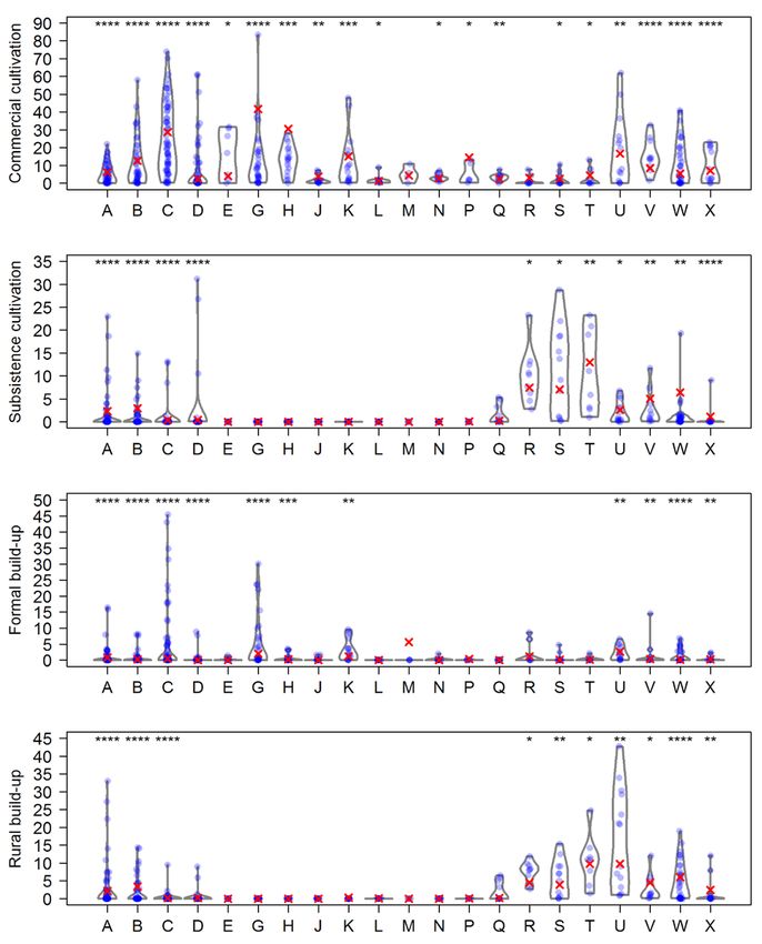
monthly mean temperature and precipitation was kept at a                           O. mossambicus and minimum and maximum temperature and
constant (mean values across the dataset) to remove any seasonal                   annual precipitation, and between C. gariepinus and maximum
effects (‘predict.lme’ from R package ‘nlme’, Pinheiro et al., 2018).              temperature (Table 1).
Next, all 442 dams were classified: firstly, according to the four                 Human land use variables had much weaker relationships with
climatic variables (annual mean, minimum and maximum                               CPUE, and were included in fewer models. Native cyprinid
temperature and annual precipitation) and, secondly, according to                  CPUE was negatively related to both types of urban build-up.
the four human land use types, natural (untransformed) land cover,                 C. gariepinus was negatively related to rural build-up and road
protected area cover, and road density. Classification was done                    density, O. mossambicus positively related to protected area and
through first conducting a principal component analysis (PCA),                     formal urban build-up and negatively related to road density, and
and then using the scores of the first components that together                    L. aeneus and L. umbratus were positively related to commercial
explain more than 80% of variation to conduct a k-means cluster                    cultivation (Table 1).
analysis limited to four clusters for simplicity (R Core Team, 2018).
                                                                                   The random effect had the strongest influence in all models,
Finally, percentage cover of the four human land use types was                     indicating large variation among dams that are not accounted for
calculated for each primary catchment (Bivand et al., 2018;                        by the variables examined in the current study (Table 1). Further,
Hijmans, 2019). Variation among dams in terms of percentage                        some total CPUE estimates are much lower than CPUE estimates
land use cover within the 5 km buffer zones was illustrated                        for specific species (e.g., L. aeneus in Armenia and Sterkfontein
with violin plots (R package ‘yarrr’, Phillips, 2017) grouped by                   Dams). Additionally, although the Tweedie models successfully
primary catchment (DWAS, 2009). Wilcoxon rank sum tests,                           estimated zero CPUE where positive samples were absent, some
the non-parametric equivalent to 1-sample t-tests, were used                       of these estimates are associated with very high uncertainty
to test whether this variation was significant. Specifically, the                  (Appendix, Table A1).
difference between land use around dams and land use in the
whole catchment was calculated, and the Wilcoxon test was used                     Cluster analysis
to compare these differences to a mean of zero. The test was only
applied when more than 5 non-zero values were available. A                         The first two components of the PCA on the four climatic variables
Holm correction was applied to the multiple p values obtained                      explain more than 86% variation, with highest factor loadings
from catchments for each land cover type (Holm, 1979).                             by annual mean temperature and minimum temperature in
                                                                                   Component 1, and highest loadings of maximum temperature
RESULTS                                                                            and annual precipitation in Component 2 (Appendix, Table A2).
                                                                                   Therefore, the k-means cluster analysis was conducted on the first
Gillnet data analysis                                                              two components. The four clusters illustrate fairly clear climate
Natural land cover was collinear with human land use cover                         zones (Fig. 2A, Table 2): (1) low winter temperatures and low
(negatively related), and annual mean temperature was collinear                    precipitation in the interior north-west of the escarpment, (2) high
with minimum and maximum temperature, and these two                                temperatures overall and high precipitation along the eastern coast
variables were therefore not included in models (variance inflation                and north-east, (3) milder temperatures and high precipitation
factors for remaining variables < 4.5). Dam surface area was not                   south along the coast and east of the escarpment, (4) high summer
included in any models after backwards stepwise selection.                         temperatures and low precipitation in the north and west.
Generally, CPUE increased in warmer months and decreased                           The first four components of the land use PCA represent more
in wetter months, except for C. carpio, O. mossambicus and                         than 81% of the variation (Appendix, Table A3) and were used
L. capensis (Table 1). Total CPUE has a weak negative relationship                 for k-means clustering. These clusters appear more geographically
with minimum temperature and native cyprinid CPUE models did                       scattered compared to the climatic clusters; however, they have clear
not include any climate covariates other than monthly temperature                  characteristics that were also reflected in the associations among
and monthly precipitation, likely because species with different                   variables in the factor loadings (Fig. 2B, Table 3 and Table A3): (1)
climate associations are combined. CPUE for individual species                     high protected area and untransformed land cover, (2) high road
indicate climate affiliations (Appendix, Fig. A1) – most species were              density and formal urban build-up indicating major cities like Cape
negatively related to minimum and maximum temperatures and                         Town, Johannesburg and Pretoria, (3) high commercial cultivation
annual precipitation, except for the positive relationships between                cover, and (4) high subsistence cultivation and rural build-up.

Table 1. Analysis of variance output from general linear mixed models with dam as random effect, to examine the relationship between CPUE and
climatic and human-related variables. The chi-square test statistics are presented, together with the level of significance depicted symbolically to
distinguish between positive and negative linear relationships, where relevant
                               Total     Cyprinids   C. carpio                  C. gariepinus     O. mossambicus L. aeneus L. capensis L. umbratus
 Monthly temperature (°C)      9.4**      14.8***        n.i.                      55.6****             8.0**     110.9**** 40.6††††       8.3**
 Monthly precipitation (mm)   12.0†††     11.0†††        n.i.                     91.9††††               5.5*     72.2††††      n.i.       7.7††
 Minimum temperature (°C)      8.1††        n.i.     11.9†††                       14.9†††               4.4*       9.9††   36.2††††        n.i.
 Maximum temperature (°C)       n.i.        n.i.         n.i.                      16.6****             7.1**     24.8††††     8.9††     17.6††††
 Annual precipitation (mm)      n.i.        n.i.         n.i.                         n.i.               4.2*     20.3††††  17.7††††      15.4†††
 Protected area (%)             n.i.        n.i.         n.i.                         n.i.               6.1*        n.i.       n.i.        n.i.
 Commercial cultivation (%)     n.i.        n.i.         n.i.                         n.i.               n.i.       6.9**       n.i.      14.9***
 Formal urban (%)               n.i.        3.9†         n.i.                         n.i.              9.5**        n.i.       n.i.        n.i.
 Rural urban (%)                n.i.        4.5†         n.i.                       10.4††                n.i         n.i       n.i.        n.i.
 Road density (km∙km−2)         n.i.         n.i         n.i.                        4.8†               9.6††        n.i.       n.i.        n.i.
 Dam identity               1 530.1**** 2 008.9**** 976.66****                   1 183.7****         1 226.6**** 960.18**** 708.7**** 1 969.0****
Positive effects: **** p < 0.0001; *** p < 0.001; ** p < 0.01; * p < 0.05; Negative effects: †††† p < 0.0001; ††† p < 0.001; †† p < 0.01; † p < 0.05;
n.i. = Not included in model with best fit

Water SA 47(3) 367–379 / Jul 2021                                                                                                                       370
https://doi.org/10.17159/wsa/2021.v47.i3.11865
Table 2. The mean and standard deviation of climatic variables in each of the four climatic k-means clusters obtained from the first two
components of a PCA
Cluster 1 Cluster 2 Cluster 3 Cluster 4
Annual mean temperature (°C) 15.6 ± 1.1 20.4 ± 1.4 16.2 ± 1.1 19.2 ± 1.4
Minimum temperature (°C) -0.4 ± 2.1 10.0 ± 2.3 5.1 ± 2.7 4.1 ± 2.0
Maximum temperature (°C) 29.8 ± 1.6 30.2 ± 1.4 26.8 ± 1.6 32.6 ± 1.7
Annual precipitation (mm) 476.8 ± 163.5 925.5 ± 164.6 717.1 ± 137.8 493.4 ± 153.1
Table 3. The mean and standard deviation of percentage coverage of land use and protected area and road density, in each of the four land use
k-means clusters obtained from the first four components of a PCA
Cluster 1 Cluster 2 Cluster 3 Cluster 4
Protected area (%) 12.0 ± 20.0 3.1 ± 5.6 3.4 ± 6.0 3.5 ± 11.4
Natural (%) 80.2 ± 14.3 38.6 ± 11.4 46.7 ± 16.1 61.1 ± 13.1
Commercial cultivation (%) 5.2 ± 5.9 4.2 ± 3.2 25.8 ± 18.2 1.9 ± 3.3
Subsistence cultivation (%) 0.6 ± 1.8 0.04 ± 0.1 0.3 ± 1.0 12.8 ± 8.7
Formal urban build-up (%) 0.8 ± 2.2 25.2 ± 9.8 2.0 ± 3.2 0.5 ± 1.1
Rural build-up (%) 1.0 ± 2.5 0.01 ± 0.01 1.0 ± 2.8 15.3 ± 10.7
Road density (km∙km−2) 2.7 ± 1.0 7.4 ± 3.0 3.6 ± 1.2 3.5 ± 1.3
Figure 2. Principal component analyses and k-means cluster analyses produced groups of dams with (A) shared climatic characteristics
summarised in Table 2 and (B) shared human-related characteristics summarised in Table 3
Water SA 47(3) 367–379 / Jul 2021 371
https://doi.org/10.17159/wsa/2021.v47.i3.11865Comparison with land use in primary catchments The findings could contribute to prioritisation of fisheries for further
intensive research to meet policy knowledge requirements and
Catchments C, D, E, G, H, J, K, L, M, N, P and Q were covered
initialise a long-term monitoring programme (Weyl et al., 2020).
by less than 1% of subsistence cultivation and rural build-up
(Fig. 3, Appendix: Table A4). Only catchments G, K, M, R and Fishery-independent gillnet CPUE was generally found to
U were covered by more than 1% cover of formal urban build- vary with monthly temperature and precipitation, likely due
up (Fig. 3, Table A4). Commercial agriculture was present in to seasonal variation in fish abundance and catchability, which
all catchments (minimum 1.36 % cover, Fig. 3, Table A4). Land should be taken into account in future fishery-independent
use cover in the 5 km zone around dams varied widely for all surveys (Pope and Willis, 1996). Further, variation in CPUE
catchments (Fig. 3). Where a Wilcoxon rank sum test was applied indicates the climatic associations of species distributions, e.g., O.
this variation was significantly different from the land cover in the mossambicus and C. gariepinus in warmer climates and L. aeneus
whole catchments (Fig. 3, Table A4). and L. capensis in cooler climates (Appendix: Fig. A1). Long-
term monitoring could reveal negative or positive responses to
DISCUSSION global warming, depending on precipitation patterns and species’
A South African inland fisheries policy and related adaptive thermal tolerances (Dallas and Rivers-Moore, 2014; Paukert et al.,
management objectives will depend on a reliable long-term 2017; Jackson et al., 2020; Kao et al., 2020). Although dam surface
supply of social-ecological data covering fisheries at a broad area is likely to be important in practice, e.g., due to variation
geographic scale, which would require developing a sustainable in total fish population size, dam area was not included in any
data collection programme (Britz et al., 2015; Tapela et al., 2015; models and is likely unimportant when selecting dams for a long-
Lynch et al., 2016; Weyl et al., 2021). The current study explored term monitoring programme. CPUE was generally weakly related
the use of easily obtainable existing data from dams across South to protected area, road density and human land use. Possible
Africa to systematically plan research and monitoring, following reasons are that gillnet-sampled dams are generally not associated
similar approaches demonstrated in previous global-scale studies with high values of human land use (more on this later), and that
(Lorenzen et al., 2016; Deines et al., 2017; Kao et al., 2020). Based the effects may be positive or negative depending on the dam and
on available fishery-independent gillnet data and GIS climatic therefore only detectable over long-term sampling (Camp et al.,
and land use data, the study revealed the variation in fish CPUE, 2020; Kao et al., 2020). Other ecological community measures
climate and land use among dams across South Africa, as well may also be better indicators of human impacts (e.g., functional
as data deficiencies where increased research is urgently needed. diversity: Jackson et al., 2020).
Figure 3. Violin and point density plots show the variation among dams in terms of percent coverage in the 5 km zone around each dam in
commercial cultivation, subsistence cultivation, formal urban build-up and rural build-up, grouped by primary catchment indicated by standard
alphabetic codes. Crosses are the percent coverage of the land use type in each catchment. Asterisks indicate Holm-corrected p values from
Wilcoxon rank sum tests indicating that land use around dams are significantly different from percentage cover in the whole catchment: * < 0.05,
** < 0.001, *** < 0.001, **** < 0.0001. Where asterisks are absent, data were too few for a test.
Water SA 47(3) 367–379 / Jul 2021 372
https://doi.org/10.17159/wsa/2021.v47.i3.11865Despite ecologically meaningful relationships between CPUE 2020; Kao et al., 2020). The South African primary catchments
and monthly and annual climate, the current FIS gillnet dataset is have distinct combinations of human land use cover generally
insufficient to generalise to unsampled dams and inform a model- indicating the types of communities and dams that are present
based survey design. All significant relationships with CPUE were (Fig. 3) and suggesting that primary catchments might be useful
weak compared to the large unexplained variation among dams units for organising sustainable management (Walmsley, 2002).
(Table 1), and there are too few data to test possible overfitting. However, as shown in the current study, a general assessment of
Additionally, high uncertainty exists for many of the CPUE the catchment might not reflect conditions specific to dams as
estimates, possibly due to insufficient repeated samples or stations there is substantial variation among dams within catchments in
(e.g. Tyefu Dam with only one sample: Appendix, Table A1), terms of land use cover in the 5 km zone.
or insufficient coverage of the climatic range relevant to the
Although the gillnet data were not sufficient to study the effect of
species (e.g. O. mossambicus, Table A1, Fig. A1). Other options
human activities, and human-related and climate characteristics
for planning large-scale monitoring include random stratified site
were not combined to classify dams, the influence of human
selection, and using statistical methods like integrated assessment
activities and environmental variation may be synergistic
modelling to combine data from different sources, e.g., combining
(Paukert et al., 2017; Jackson et al., 2020; Kao et al., 2020). For
FIS and fishery-dependent survey (FDS) data (Lorenzen et al.,
2016; Deines et al., 2017; Kao et al., 2020). Additionally, FDS data example, clean water supply could increase the resilience of
like records from recreational or subsistence fishing may be better aquatic ecosystems to a changing climate and increased human
for monitoring species that are not sampled well with gillnets, like activities (Dallas and Rivers-Moore, 2014; Kao et al., 2020).
common carp Cyprinus carpio and largemouth bass Micropterus However, precipitation is projected to decrease, especially in
salmoides (Winker, 2010; McCafferty, 2012). the southwestern winter rainfall region of South Africa, with a
general increase in rainfall intensity and extreme flood or drought
The large-scale classification approach may be useful in the events compounding the stresses from agricultural intensification
absence of, or during the early development stages of, a long-term and urban expansion on aquatic ecosystems (Dallas and Rivers-
fishery monitoring dataset, by revealing high-value or high-risk Moore et al., 2014; Archer et al., 2018; Jackson et al., 2020). Dams
dams to prioritise for intensive data collection. The current study are increasingly important as refuges for fish during droughts,
revealed groups of dams with shared climatic characteristics that while competing with human water consumption (Beatty et
seem to associate with certain primary catchments due to the al., 2017). Sustainable economic development is much needed
strong effect of the escarpment (Figs 1 and 2A). Although the in socioeconomically underdeveloped areas, and could ensure
gillnet models cannot generalise CPUE estimates to unsampled increased water use efficiency and quality, and sanitation access
dams, these climate clusters roughly indicate dams where certain to reduce pollution (Kao et al., 2020). However, unsustainable
fish species could thrive, or dams where fish populations should human land use intensification or poorly planned development
be monitored for vulnerability to climate change (Britz et al., 2015; could affect aquatic ecosystems through increased erosion,
Jackson et al., 2020; Kao et al., 2020). Dominant species’ CPUE sedimentation, eutrophication and heavy metal pollution, and
estimates broadly match the climate clusters, with comparatively decrease fish population resilience and fishery product quality and
higher CPUE for L. aeneus and L. capensis associated with the safety, possibly further marginalising those most dependent on
relatively cooler Cluster 1, whereas O. mossambicus are largely the fishery (Papu-Zamxaka et al., 2010; Jooste et al., 2014; Jackson
present in Cluster 4 where maximum temperature is higher et al., 2020; Kao et al., 2020). This further highlights the need to
(Table 2, Fig. 2A and Appendix: Fig. A1). Dams in Cluster 2 (high study the social-ecological dynamics of fisheries and incorporate
temperature and high rainfall) are currently represented by only human activity, social and economic data into fishery survey and
three dams with gillnet data, which could bias predictions of fish monitoring programmes (Beard et al., 2011; Hara and Backeberg,
species distributions. 2014; Tapela et al., 2015).
Groups of dams with shared human-related characteristics are
geographically more scattered (Fig. 2B); however, they have CONCLUSIONS
very distinct characteristics, signifying (1) dams in remote The current study demonstrates how available data, like the FIS
untransformed and protected areas, (2) dams close to towns gillnet data and GIS data evaluated here, could be used to streamline
and cities, (3) dams surrounded by commercial cultivation, and the development of a sustainable data collection programme for
(4) dams close to rural communities depending on subsistence a South African inland fisheries policy, while also revealing data
cultivation (Table 3). Clusters 1 and 4 may be suitable targets gaps where increased research should be focused. Broad-scale
for recreational fishery management and small-scale fishery classification of dams by climate and land use associations is a
development, respectively, depending on the population size of method for rapidly prioritising dams for further dam-specific
the dominant fish species (Weyl et al., 2007). Of the 44 gillnet- data collection. Dam-specific research should include assessing
sampled dams, 32 are associated with Cluster 1, and dams fishery potential and current fishing activity, and identifying
characterised by more substantial transformed land cover are dams that are unsuitable for fishing (e.g. polluted dams), thereby
currently very poorly represented. Of the 6 gillnet-sampled dams further refining the selection of dams for fishery management and
associated with Cluster 4, only Dimbaza dam is estimated to have monitoring (Papu-Zamxaka et al., 2010; Jooste et al., 2014; Weyl
a fairly high L. umbratus CPUE (Appendix, Table A1). More et al. 2021). The classification analysis identified dams that are
fishery data is needed from dams associated with subsistence likely important for small-scale and subsistence fisheries, which
communities through additional gillnet samples, or by obtaining require increased research effort (Hara and Backeberg, 2014;
catch size records from the local fishers (see e.g. Appendix 1 in Tapela et al., 2015). However, dam-specific research may identify
Tapela et al., 2015). many dams with mixed recreational, subsistence and small-scale
fisheries that require support for multiple stakeholders (Smith et
The current study focused on a 5 km zone around each individual
al., 2005; Ellender et al., 2009; Weyl et al. 2021).
dam to better represent access. However, the influence of human
activities and climate on waterbodies is often examined at a Before the FIS gillnet dataset would be useful for modelling
catchment level, as dam-specific data are often scarce, and aquatic general patterns or model-based sampling design, it should be
ecosystems are influenced by human activities and climate in expanded with recurrent samples from dams representing the
whole river drainage basins (Jooste et al., 2014; Jackson et al., full range of climate and land use characteristics indicated by
Water SA 47(3) 367–379 / Jul 2021 373
https://doi.org/10.17159/wsa/2021.v47.i3.11865the classification analyses. Further, the predictive capability of BATES B, MAECHLER M, BOLKER B and WALKER S (2015) Fitting
models could be improved by consistently recording additional linear mixed-effects models using lme4. J. Stat. Softw. 67 (1) 1–48.
variables that influence CPUE, other than seasonal climate. For https://doi.org/10.18637/jss.v067.i01
example, fish abundance could be affected by fishing pressure, BEARD TD, ARLINHAUS R, COOKE SJ, MCINTYRE PB, DE SILVA
S, BARTLEY D and COWX IG (2011) Ecosystem approach to inland
whereas catchability could be affected by turbidity, water
fisheries: research needs and implementation strategies. Biol. Letters.
temperature and time of day (Vašek et al., 2009; Latour, 2016;
7 (4) 481–483. https://doi.org/10.1098/rsbl.2011.0046
Weyl et al., 2021). Other possible methods to obtain CPUE data BEATTY S, ALLEN M, LYMBERY A, JORDAAN MS, MORGAN D,
should also be examined, including random stratified survey IMPSON D, MARR S, EBNER B and WEYL OLF (2017) Rethinking
design and combining catch data from various sources, including refuges: Implications of climate change for dam busting. Biol.
fishery-dependent data (Paukert et al., 2017; Camp et al., 2020). Conserv. 209 188–195. https://doi.org/10.1016/j.biocon.2017.02.007
Moreover, long-term monitoring can be iteratively improved by BIVAND R, KEITT T and ROWLINGSON B (2018) rgdal: Bindings for
periodically revising the survey design and sampling methods the ‘Geospatial’ Data Abstraction Library. R package version 1.3-6.
according to data insufficiencies revealed by models based on BONAR SA and HUBERT WA (2002) Standard sampling of inland fish:
previously collected data (Guisan et al., 2006). Therefore, the cost benefits, challenges, and a call for action. Fisheries. 27 10–16. https://
and effort spent to develop and maintain a long-term monitoring doi.org/10.1577/1548-8446(2002)0272.0.co;2
BRITZ P (2015) The history of South African inland fisheries policy
programme will return increasingly valuable data that are
with governance recommendations for the democratic era. Water
essential for adaptive management responses to environmental
SA. 41 (5) 624–632. https://doi.org/10.4314/wsa.v41i5.05
and socioeconomic change. BRITZ PJ, HARA MM, WEYL OLF, TAPELA BN and ROUHANI QA
(2015) Scoping study on the development and sustainable utilisation
ACKNOWLEDGEMENTS of inland fisheries in South Africa Volume 1: Research report. WRC
Report No. TT 615/1/14. Water Research Commission, Pretoria.
The helpful comments from two anonymous reviewers were very
CAMP EV, KAEMING MA, AHRENS RNM, POTTS WM, PINE
much appreciated. This study was supported by the infrastructure
WE, WEYL OLF and POPE KL (2020) Resilience management
provided by the SAIAB Research Platform and the funding for conservation of inland recreational fisheries. Front. Ecol. Evol.
channelled through the NRF–SAIAB Institutional Support system 7 498. https://doi.org/10.3389/fevo.2019.00498
as well as support from the National Research Foundation – South CD:NGI (1998) Roads: 1:500 000 Topographical Edition of South
African Research Chairs Initiative of the Department of Science Africa. Chief Directorate: National Geo-Spatial Information,
and Innovation (Grant No. 110507) and the NRF Professional Department of Agriculture, Rural Development and Land Reform.
Development Programme (Grant No. 104911). Any opinion, http://daffarcgis.nda.agric.za/portal/home/
finding and conclusion or recommendation expressed in this DALLAS HF and RIVERS-MOORE N (2014) Ecological consequences
material is that of the authors and the NRF do not accept any of global climate change for freshwater ecosystems in South Africa. S.
liability in this regard. Afr. J. Sci. 110 (5–6) 1–11. https://doi.org/10.1590/sajs.2014/20130274
DEA (Department of Environmental Affairs, South Africa) (2015)
South African National Land Cover, Department of Environmental
AUTHOR CONTRIBUTIONS
Affairs, Pretoria. https://egis.environment.gov.za/data_egis/data_
SH conceptualised the study and developed the methodology, download/current
analysed and interpreted the data and wrote the initial draft. DEINES AM, BUNNELL DB, ROGERS MW, BENNION D,
OLFW supplied the gillnet data, contributed to the study concept WOELMER W, SAYERS MJ, GRIMM AG, SHUCHMAN RA,
and edited the manuscript. RAYMER ZB, BROOKS CN, MYCHEK-LONDER JG, TAYLOR W
and BEARD TD (2017) The contribution of lakes to global inland
fisheries harvest. Front. Ecol. Environ. 15 (6) 293–298. https://doi.
ORCID
org/10.1002/fee.1503
S Hugo DWA (Department of Water Affairs, South Africa) (2009) Catchments
https://orcid.org/0000-0001-8636-3985 of South Africa. Department of Water Affairs, Pretoria. https://doi.
org/10.15493/SARVA.DWS.10000003
OLF Weyl DWA (Department of Water Affairs, South Africa) (2011) Dams and
https://orcid.org/0000-0002-8935-3296 lakes, electronic dataset. Department of Water Affairs, Pretoria.
https://doi.org/10.15493/SARVA.DWS.10000001
REFERENCES ELLENDER BR, WEYL OLF and WINKER H (2009) Who uses the fishery
resources in South Africa’s largest impoundment? Characterising
ANDREW TG, ROUHANI QA and SETI SJ (2000) Can small-scale
subsistence and recreational fishing sectors on Lake Gariep. Water SA.
fisheries contribute to poverty alleviation in traditionally non-
35 (5) 677–682. https://doi.org/10.4314/wsa.v35i5.49194
fishing communities in South Africa? Afr. J. Aquat. Sci. 25 (1) 50–55.
FOX J and WEISBERG S (2019) An R Companion to Applied Regression
https://doi.org/10.2989/160859100780177938
(3rd edn). Sage Publications, Thousand Oaks CA.
ARCHER E, ENGELBRECHT F, HÄNSLER A, LANDMAN W,
TADROSS M and HELMSCHROT J (2018) Seasonal prediction and GUISAN A, BROENNIMANN O, ENGLER R, VUST M, YOCCOZ NG,
regional climate projections for southern Africa. In: Revermann LEHMANN A and ZIMMERMANN NE (2005) Using niche-based
R, Krewenka KM, Schmiedel U, Olwoch JM, Helmschrot J and models to improve the sampling of rare species. Conserv. Biol. 20 (2)
Jürgens N (eds.) Climate Change and Adaptive Land Management in 501–511. https://doi.org/10.1111/j.1523-1739.2006.00354.x
Southern Africa – Assessments, Changes, Challenges, and Solutions. HARA MM and BACKEBERG GR (2014) An institutional approach for
Klaus Hess Publishers, Göttingen & Windhoek. https://doi.org/ developing South African inland freshwater fisheries for improved
10.7809/b-e.00296 food security and rural livelihoods. Water SA. 40 (2) 277–286.
BAKER MR, PALSSON W, ZIMMERMAN M and ROOPER CN https://doi.org/10.4314/wsa.v40i2.10
(2019) Model of trawlable area using benthic terrain and HIJMANS RJ, CAMERON SE, PARRA JL, JONES PG and JARVIS
oceanographic variables–Informing survey design and habitat A (2005) Very high resolution interpolated climate surfaces for
maps in the Gulf of Alaska. Fish. Oceanogr. 28 (6) 629–657. https:// global land areas. Int. J. Climatol. 25 (15) 1965–1978. https://doi.
doi.org/10.1111/fog.12442 org/10.1002/joc.1276
BARKHUIZEN LM, WEYL OLF and VAN AS JG (2016) A qualitative HIJMANS RJ (2019) raster: Geographic Data Analysis and Modeling.
and quantitative analysis of historic commercial fisheries in the Free R package version 2.8-19.
State Province in South Africa. Water SA. 42 (4) 601–605. https:// HOLM S (1979) A simple sequentially rejective multiple test procedure.
doi.org/10.4314/wsa.v42i4.10 Scand. J. Stat. 6 65–70.
Water SA 47(3) 367–379 / Jul 2021 374
https://doi.org/10.17159/wsa/2021.v47.i3.11865JACKSON MC, FOURIE HE, DALU T, WOODFORD DJ, WASSERMAN PINHEIRO J, BATES D, DEBROY S, SARKAR D and R CORE TEAM RJ, ZENGEYA TA, ELLENDER BR, KIMBERG PK, JORDAAN MS, (2018) nlme: Linear and nonlinear mixed effects models. R package CHIMIMBA CT and WEYL OLF (2020) Food web properties vary version 3.1-137. with climate and land use in South African streams. Funct. Ecol. 34 POPE KL and WILLIS DW (1996) Seasonal influences on freshwater (8) 1653–1665. https://doi.org/10.1111/1365-2435.13601 fisheries sampling data. Rev. Fish. Sci. 4 (1) 57–73. https://doi. JOOSTE A, MARR SM, ADDO-BEDIAKO A and LUUS-POWELL org/10.1080/10641269609388578 WJ (2014) Metal bioaccumulation in the fish of the Olifants River, QGIS DEVELOPMENT TEAM (2018) QGIS Geographic Information Limpopo province, South Africa, and the associated human System. Open Source Geospatial Foundation Project. URL: http:// health risk: a case study of rednose labeo Labeo rosae from two qgis.osgeo.org impoundments. Afr. J. Aquat. Sci. 39 (3) 271–277. https://doi.org/10. R CORE TEAM (2018) R: A language and environment for statistical 2989/16085914.2014.945989 computing. R Foundation for Statistical Computing, Vienna, KAO Y, ROGERS MW, BUNNELL DB, COWX IG, QIAN SS, Austria. https://www.R-project.org/ ANNEVILLE O, BEARD TD, BRINKER A, BRITTON JR, RIVERS-MOORE NA, GOODMAN PS and NEL JL (2011) Scale-based CHURA-CRUZ R and co-authors (2020) Effects of climate and freshwater conservation planning: towards protecting freshwater land-use changes on fish catches across lakes at a global scale. Nat. biodiversity in KwaZulu-Natal, South Africa. Freshwater Biol. Commun. 11 2526. https://doi.org/10.1038/s41467-020-14624-2 56 125–141. https://doi.org/10.1111/j.1365-2427.2010.02387.x LATOUR RJ (2016) Explaining patterns of pelagic fish abundance in the SANPARKS (2004) Archived NSBA Terrestrial Protected Areas vector Sacramento-San Joaquin Delta. Estuaries Coast. 39 233–247. https:// geospatial dataset. South African National Parks, Pretoria. URL: doi.org/10.1007/s12237-015-9968-9 http://bgis.sanbi.org/SpatialDataset/Detail/150 LORENZEN K, COWX LG, ENTSUA-MENSAH REM, LESTER SHONO H (2008) Application of the Tweedie distribution to zero- NP, KOEHN JD, RANDALL RG, SO N, BONAR SA, BUNNELL catch data in CPUE analysis. Fish. Res. 93 (1–2) 154–162. https://doi. DB, VENTURELLI P, BOWER SD and COOKE SJ (2016) Stock org/10.1016/j.fishres.2008.03.006 assessment in inland fisheries: a foundation for sustainable use SMITH LED, KHOA N and LORENZEN K (2005) Livelihood function and conservation. Rev. Fish Biol. Fisher. 26 405–440. https://doi. of inland fisheries: policy implications in developing countries. org/10.1007/s11160-016-9435-0 Water Policy. 7 (4) 359–383. https://doi.org/10.2166/wp.2005.0023 LYNCH AJ, COOKE SJ, DEINES AM, BOWER SD, BUNNEL DB, TAPELA BN, BRITZ PJ and ROUHANI QA (2015) Scoping study on the COWX IG, NGUYEN VM, NOHNER J, PHOUTHAVONG K, development and sustainable utilisation of inland fisheries in South RILEY B, ROGERS MW, TAYLOR WW, WOELMER W, YOUN S Africa Volume 2: Case studies of small-scale inland fisheries. WRC and BEARD TD (2016) The social, economic, and environmental Report No. TT 615/2/14. Water Research Commission, Pretoria. importance of inland fisheries. Environ. Rev. 24 (2) 115–121. https:// TWEEDIE MCK (1984) An index which distinguishes between some doi.org/10.1139/er-2015-0064 important exponential families. In: Ghosh JK and Roy J (eds.) MCCAFFERTY JR (2012) An assessment of inland fisheries in South Statistics: Applications and New Directions. Proceedings of the Indian Africa using fisheries-dependent and fisheries-independent data Statistical Institute Golden Jubilee International Conference. Indian sources. PhD thesis, Rhodes University. Statistical Institute, Calcutta. MCCAFFERTY JR, ELLENDER BR, WEYL OLF and BRITZ PJ (2012) VAŠEKA M, KUBEČKA J, ČECH M, DRAŠTIK V, MATĔNA J, The use of water resources for inland fisheries in South Africa. Water MRKVIČKA T, PETERKA J and PRCHALOVÁ M (2009) Diel SA. 38 (2) 327–344. https://doi.org/10.4314/wsa.v38i2.18 variation in gillnet catches and vertical distribution of pelagic fishes PAPU-ZAMXAKA V, MATHEE A, HARPHAM T, BARNES B, in a stratified European reservoir. Fish. Res. 96 64–69. https://doi. RÖLLIN H, LYONS M, JORDAAN W and CLOETE M (2010) org/10.1016/j.fishres.2008.09.010 Elevated mercury exposure in communities living alongside the WALMSLEY JJ (2002) Framework for measuring sustainable develop- Inanda Dam, South Africa. J. Environ. Monitor. 12 (2) 472–477. ment in catchment systems. Environ. Manage. 29 195–206. https:// https://doi.org/10.1039/b917452d doi.org/10.1007/s00267-001-0020-4 PAUKERT CP, LYNCH AJ, BEARD TD, YUSHUN C, COOKE SJ, WEYL OLF, BARKHUIZEN L, CHRISTISON K, DALU T, COOPERMAN MS, COWX IG, IBENGWE L, INFANTE DM, HLUNGWANI HA, IMPSON D, SANKAR K, MANDRAK NE, MYERS BJE, HÒA PHÚ N and WINFIELD IJ (2017) Designing a MARR SM, SARA JR and co-authors (2021) Ten research questions global assessment of climate change on inland fish and fisheries: to support South Africa’s Inland Fisheries Policy. Afr. J. Aquat. Sci. knowns and needs. Rev. Fish Biol. Fisher. 27 (2) 393–409. https://doi. 46 (1) 1–10. https://doi.org/10.2989/16085914.2020.1822774 org/10.1007/s11160-017-9477-y WEYL OLF, POTTS W, ROUHANI QA and BRITZ P (2007) The need PEEL D, BRAVINGTON MV, KELLY N, WOOD SN and KNUCKEY I for inland fisheries policy in South Africa: a case study of the North (2012) A model-based approach to designing a fishery-independent West Province. Water SA. 33 (4) 497–504. survey. J. Agr. Biol. Envir. St. 18 (1) 1–21. https://doi.org/10.1007/ WINKER H (2010) Post-impoundment population dynamics of non- s13253-012-0114-x native common carp Cyprinus carpio in relation to two large PHILLIPS N (2017) yarrr: a companion to the e-book “YaRrr!: The native cyprinids in Lake Gariep, South Africa. PhD thesis, Rhodes pirate’s guide to R”. R package version 0.1.5. University. Water SA 47(3) 367–379 / Jul 2021 375 https://doi.org/10.17159/wsa/2021.v47.i3.11865
APPENDIX

Figure A1. The location of the dams listed in Table A1, with CPUE (kg∙month−1∙sampling station−1) estimates indicated and primary catchments
delineated. The CPUE colour scales are on the logarithmic scale to better distinguish visually, with black indicating zero

Water SA 47(3) 367–379 / Jul 2021                                                                                                      376
https://doi.org/10.17159/wsa/2021.v47.i3.11865
Table A1. The predicted catch per unit effort (CPUE, kg∙month−1∙sampling station−1) from each dam derived from models presented in Table 1 in
the main text, where monthly temperature and precipitation were kept constant (at mean value across dataset). Lower and upper bounds of the
95% confidence intervals are in brackets
 Catchment                 Total           Native          Cyprinus        Clarias        Oreochromis       Labeobarbus         Labeo            Labeo
 and dam                                  cyprinids         carpio        gariepinus      mossambicus         aeneus           capensis         umbratus
 A Bospoort                 4.05              0.00            0.69            1.39             1.47              0.00             0.00             0.00
                        (2.08; 7.88)      (0.00; 0.00)    (0.22; 2.15)    (0.48; 4.00)     (0.81; 2.64)      (0.00; 3.99)     (0.00; 0.48)    (0.00; > 95.00)
 A Koster                  8.50               0.70            0.21            6.48             1.12              0.00             0.00             0.00
                       (4.37; 16.54)      (0.24; 1.98)    (0.05; 0.98)    (3.06; 13.71)    (0.57; 2.20)      (0.00; 0.40)     (0.00; 0.30)    (0.00; > 95.00)
 A Lindleyspoort           6.83               1.46            0.10            5.09              0.25             0.00             0.00             0.00
                       (3.87; 12.05)      (0.67; 3.19)    (0.02; 0.46)    (2.60; 9.96)      (0.11; 0.59)     (0.00; 0.69)     (0.00; 0.27)    (0.00; > 95.00)
 A Madikwe                 11.71              1.05            0.00            9.01             0.20              0.00             0.00             0.00
                       (6.64; 20.65)      (0.46; 2.39)    (0.00; 0.60)    (5.20; 15.63)    (0.08; 0.52)      (0.00; 1.82)     (0.00; 0.19)    (0.00; > 95.00)
 A Molatedi                14.51              3.37            0.01            5.29             2.76              0.00             0.00             0.00
                       (8.22; 25.59)      (1.75; 6.50)    (0.00; 0.11)    (3.03; 9.23)     (1.95; 3.89)      (0.00; 2.09)     (0.00; 0.20)    (0.00; > 95.00)
 A Ngotwane                14.21              2.27            0.00            9.45             0.00              0.00             0.00             0.00
                       (8.06; 25.07)      (1.09; 4.72)    (0.00; 0.59)    (5.53; 16.14)    (0.00; 13.82)     (0.00; 0.05)     (0.00; 0.02)     (0.00; 33.47)
 A Roodekopjes             14.08             6.13             0.29            4.83             1.75              0.00             0.00             0.00
                       (7.98; 24.83)     (3.34; 11.27)    (0.09; 0.88)    (2.63; 8.86)     (1.16; 2.64)      (0.00; 1.30)     (0.00; 0.23)     (0.00; 94.12)
 A Vaalkop                 29.39             11.93            0.00            10.12            5.41              0.00             0.00             0.00
                       (16.66; 51.84)    (6.74; 21.13)    (0.00; 0.57)    (5.91; 17.36)    (4.02; 7.28)      (0.00; 3.14)     (0.00; 0.31)    (0.00; > 95.00)
 B Flag Boshielo            3.15              1.98            0.01            0.15             0.63              0.00             0.00             0.00
                        (2.56; 3.88)      (1.53; 2.57)    (0.01; 0.03)    (0.09; 0.25)     (0.50; 0.78)      (0.00; 0.00)     (0.00; 0.00)     (0.00; 0.64)
 B Loskop                  12.50              2.94            0.00            1.00             10.33             0.00             0.00             0.00
                       (6.64; 23.54)      (1.56; 5.53)    (0.00; 0.30)    (0.51; 1.95)     (8.57; 12.45)     (0.00; 0.08)     (0.00; 0.01)     (0.00; 12.47)
 C Allemanskraal           7.72              4.75             0.41            2.67             0.00              1.16             0.92             2.40
                       (3.74; 15.97)     (2.23; 10.10)    (0.13; 1.28)    (1.13; 6.34)     (0.00; 33.24)     (0.52; 2.61)     (0.44; 1.91)     (1.27; 4.54)
 C Bloemhoek              42.66             36.92             0.43            5.35             0.00              0.63             11.84           25.43
                      (20.63; 88.23)    (18.59; 73.35)    (0.09; 2.13)    (1.86; 15.40)   (0.00; > 33.30)    (0.18; 2.23)     (6.60; 21.25)   (15.65; 41.33)
 C Bloemhoff               15.12              2.16            6.13            5.38             0.00              0.78             1.11             0.48
                       (7.31; 31.27)      (0.94; 5.00)    (3.43; 10.98)   (2.78; 10.43)    (0.00; 26.52)     (0.36; 1.69)     (0.54; 2.27)     (0.18; 1.28)
 C Jimmy Roos              56.17             51.02            0.00            7.12             0.00              0.00             0.00            53.02
                      (27.77; 113.61)    (27.23; 95.59)   (0.00; 1.63)    (2.93; 17.31)   (0.00; > 33.30)    (0.00; 0.06)     (0.00; 0.02)    (37.02; 75.93)
 C Kalkfontein             31.89            27.67             1.05            2.07             0.00              2.64             4.44            15.00
                       (15.42; 65.94)   (15.76; 48.58)    (0.42; 2.59)    (0.98; 4.39)    (0.00; > 33.30)    (1.57; 4.44)     (2.56; 7.67)    (10.83; 20.76)
 C Koppies                 53.40            45.30             0.78            17.97            0.00             43.56             2.40            27.78
                      (25.82; 110.42)   (26.20; 78.34)    (0.29; 2.07)    (9.83; 32.84)   (0.00; > 33.30)   (27.45; 69.12)    (1.31; 4.40)    (19.98; 38.61)
 C Krugersdrift            15.68             10.47            1.21            2.85             0.00              0.60             1.77             8.27
                       (9.40; 26.13)     (6.56; 16.72)    (0.65; 2.27)    (1.66; 4.90)     (0.00; 1.71)      (0.34; 1.05)     (1.11; 2.82)     (6.15; 11.11)
 C Metsi Matso              1.64              0.00            0.00            0.00             0.79              0.00             0.00             0.00
                        (0.81; 3.32)      (0.00; 0.01)    (0.00; 2.70)    (0.00; 7.69)     (0.34; 1.83)      (0.00; 1.75)     (0.00; 0.05)    (0.00; > 95.00)
 C Mockes                  16.03              3.07            0.00            11.63            0.00              0.00             1.07             2.25
                       (7.93; 32.43)      (1.18; 7.93)    (0.00; 1.86)    (5.45; 24.81)   (0.00; > 33.30)     (0.00; 0.11)    (0.43; 2.69)     (0.90; 5.58)
 C Moutloasi               12.59             7.60            0.54             3.63             0.00              0.00             5.51             2.59
                       (7.56; 20.99)     (4.29; 13.45)    (0.21; 1.41)    (1.77; 7.44)    (0.00; > 33.30)    (0.00; 0.02)     (3.57; 8.50)     (1.44; 4.64)
 C Rustfontein             15.28             9.09             1.28            4.14             0.00               2.25            0.97             5.48
                       (9.17; 25.48)     (5.61; 14.73)    (0.69; 2.37)    (2.45; 7.02)    (0.00; > 33.30)     (1.41; 3.59)    (0.58; 1.64)     (3.87; 7.76)
 C Serfontein               3.88              0.00           0.00             4.65             0.00              0.00             0.00             0.00
                        (1.92; 7.86)      (0.00; 0.00)    (0.00; 2.11)    (1.61; 13.42)   (0.00; > 33.30)    (0.00; 0.17)     (0.00; 0.04)     (0.00; 34.77)
 C Sterkfontein            18.17            16.42             0.11            6.50             0.00              99.70            2.22             2.91
                       (10.90; 30.29)   (10.28; 26.23)    (0.04; 0.35)    (3.26; 12.99)    (0.00; 9.05)     (68.95; 144.16)   (1.45; 3.39)     (1.71; 4.94)
 C Taung                   15.22             11.08            0.20            3.39             0.00              6.37             0.98             0.27
                       (7.96; 29.10)     (5.83; 21.05)    (0.05; 0.84)    (1.57; 7.32)    (0.00; > 33.30)    (3.84; 10.57)    (0.48; 2.04)     (0.08; 0.92)
 C Tierpoort               43.33             14.97            9.50            16.61            0.00              3.34             0.70             9.34
                       (21.42; 87.64)    (7.09; 31.58)    (4.65; 19.40)   (8.49; 32.50)    (0.00; 0.07)      (1.64; 6.83)     (0.26; 1.88)     (5.23; 16.68)
 D Armenia                 74.41          72.03               3.96            3.92             0.00              91.63             3.49            7.11
                      (36.79; 150.51) (39.36; 131.81)     (1.63; 9.63)    (1.26; 12.15)   (0.00; > 33.30)   (57.83; 145.19)    (1.71; 7.10)    (3.55; 14.26)
 D Egmont                   16.30            15.05            0.55            2.51             0.00              13.11            1.07             2.35
                        (9.78; 27.18)    (9.32; 24.30)    (0.24; 1.27)    (1.25; 5.01)    (0.00; > 33.30)    (8.95; 19.21)    (0.62; 1.85)     (1.41; 3.94)
 D Gariep                  16.81             14.62            0.53            1.38             0.00              5.84             3.96             0.17
                       (12.13; 23.29)    (11.17; 19.14)   (0.34; 0.82)    (0.93; 2.03)     (0.00; 5.29)      (4.72; 7.23)     (3.20; 4.91)     (0.10; 0.28)

Water SA 47(3) 367–379 / Jul 2021                                                                                                                        377
https://doi.org/10.17159/wsa/2021.v47.i3.11865
You can also read