Radio Observations of the Solar Eclipse on 20 March 2015
←
→
Page content transcription
If your browser does not render page correctly, please read the page content below
Radio Observations of the Solar Eclipse on 20 March 2015

                                   Joachim Köppen, DF3GJ,
                                   for the Team at DL0SHF,
                                   Inst.Theor.Physik u.Astrophysik, Univ.Kiel

The Raw Data
Observations are done with the DL0SHF parabolic antennas on 1.3, 2.3, 8.2, and 10 GHz. The Sun is
automatically tracked by the pointing software, and the solar noise is measured by HP437B power
meters, after passing through a chain of filters and amplifiers on the signal frequency with a 2 MHz
bandwidth. Below are shown the entire raw data. On 1.3 and 10 GHz the signal power is measured
every 2 seconds, and is recorded in a file along with the time and the present azimuth and elevation. On
2.3 and 8.2 GHz, measurements are taken and recorded every 0.5 second.

Fig. 1 The raw data from 1.3 GHz. Before and after the solar measurements flux calibrations with
ground radiation and a sky profile (elevations = 15, 20, 25, 30, 40, 60°) are taken. The strong level
variations before UT 07:40 are tests of the tracking arrangement.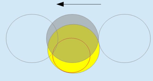
Fig. 2 The raw data from 2.3 GHz. Before the solar measurements, the power meter zero level is set by
pointing at the empty sky at elevation 45°. During the observing run, a slow and gradual decrease of
the gain is noticed. The origin is not yet known.

Fig. 3 The raw data from 8.2 GHz. Before the solar measurements, the power meter zero level is set by
pointing at the empty sky at elevation 45°. The data contains a number of jumps in the level, and also
quite strong fluctuations which are nearly periodic. Note also that the minimum signal occurs near UT
0936, about 10 min before the maximum covering of the Sun (cf. Fig.4). This is undoubtedly due to the
narrow antenna beam pointing to a position West of the centre of the solar disk.
Fig. 4 The raw data from 10 GHz. Before and after the solar measurements flux calibrations with
ground radiation are taken as well as sky profiles (elevations = 10, 15, 20, 25, 30, 40, 60°).

Data Reduction
The antenna beams on 1.3 and 2.3 GHz are wider than the solar disk, so that the entire emission is
captured. As will be seen in Fig.8, the signals' time dependence are well bracketed by the times of first
and last contact.

However, it turns out that on 8.2 GHz the minimum signal level occurs near UT 09:36, earlier than the
moment of the largest covering of the Sun, at UT 09:46 (computed for Rönne from:
http://eclipse.gsfc.nasa.gov/eclipse.html). Evidently, the narrow antenna beam (0.4° width) is not well
centered on the solar disk. As the Moon moves with respect to the Sun by almost 2 solar disk diametres
between first and last contact (at UT 08:38 and 10:56, respectively), a time difference of 10 min means
that the centre of the antenna beam was displaced from the disk centre by 0.14° toward the Western
limb, parallel to the Moon's movement. Furthermore, that the minimum signal on 8 GHz is not as deep
as the one on 10 GHz indicates that the antenna beam is displaced away from the path of the Moon's
direction. From the flux curve one can roughly estimate the situation depicted in Fig.5.

Similarly, at 10 GHz the minimum signal happens about 2 min after maximum eclipse. This means that
the antenna beam is displaced by 0.016° towards the Eastern limb, which is well within the accuracy of
the tracking system and the current pointing correction. As the antenna beam is smaller than the Sun's
disk, the flux would have gone to zero, if the beam was well centered in the vertical direction. The
situation displayed in Fig.6 is a reasonable guess for a somewhat lower minimum flux than expected
from the obscuration of the whole solar disk.

To aid the comparison with the other frequencies in all following figures, we advanced the 8.2 GHz
data by 7.5 min and delayed the 10 GHz data by 3 min with respect to the low frequencies..
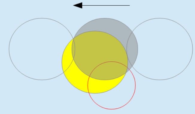
Fig. 5 The geometrical situation near the minimum signal on 8.2 GHz received by the antenna beam
(red circle).

Fig. 6 Like Fig.5, but for 10 GHz.

For all data sets a box car smoothing over 30 data points is applied. The rather strong and nearly
periodic level variations in the 8.2 GHz data are completely suppressed, and this smoothing is also
useful in the other data.

The sudden level jumps in the 8.2 GHz data are treated in a manual way: all powers after UT 10:10 are
increased by 1.0 dB, which gives very satisfactory results. Also, the depression around UT 08:50 is
partially removed by adding 0.5 dB.

The overall tendency of the 2.3 GHz level to drop is removed by manually estimating the run of the
true maximum solar level, and normalizing the data to that level. As the resulting curve agrees very
well with the 1.3 GHz data, this can be taken as an assurance that this adhoc approach models quite
well the actual gain variation. This approach is also used to compensate the slight level variations at the
other frequencies.
For the 1.3 and 10 GHz data full flux calibrations and sky noise measurements are available. Thus
system temperature and zenith temperature are determined by fitting a straight line to the measured
linear values as a function of the airmass, i.e. 1/sin(elevation). One example is shown in Fig.7.

                                   System temperature [K]            Zenith temperature [K]
1.3 GHz before                     59.4                              5.0
1.3 GHz after                      47.4                              6.4
1.3 GHz adopted                    50.0                              5.0
10 GHz before                      96.6                              4.4
10 GHz after                       91.4                              5.0
10 GHz adopted                     95.0                              5.0

Fig. 7 System temperature and zenith temperature are determined from the empty sky noise measured
at a number of elevations.

While the system temperature for 1.3 GHz agrees well with earlier measurements, the value obtained
for 10 GHz is substantially lower that previously found values of about 150 K. This issue needs further
attention.

For 2.3 and 8.2 GHz only the zero-point of the HP437B instrument is set by measuring the empty sky.
The system temperatures are assumed as 50 and 90 K, respectively and a zenith temperature of 5.0 K.

Antenna temperatures are derived from measured (linear) power:

   p = a (TA + TSYS + TCMB + TSKY(el))

with TSKY(el) = TZEN/sin(el) from the plane-parallel model of the Earth atmosphere, and the cosmic
microwave background TCMB = 2.7 K.
For 1.3 and 10 GHz, the factor a is derived from the flux calibration pCAL = a (TCAL + TSYS) with the ground temperature TCAL = 290 K. For 2.3 and 8.2 GHz, a is derived from the zero-setting using the sky noise at 45° elevation: pZERO = a (TSYS + TCMB + TSKY(45°)) In this way, the linear powers p = 10dB/10 for all individual measurements are converted into antenna temperatures, which are a measure of the flux received from the Sun by the antenna. Results Fig. 8 The relative powers during the eclipse. The vertical blue lines mark (from left) the first contact predicted of the optical eclipse, maximum obscuration, and last contact. The colours are the same as in the corresponding figures of the raw data: red (1.3 GHz), blue (2.3 GHz), green (8.2 GHz), black (10 GHz). The most remarkable feature is already noticed during the observations: the drop of the signal level started on lower frequencies earlier than on the higher ones. The 1.3 and 2.3 GHz curve lie very close together – despite the gradual drop in the gain in the 2.3 GHz raw data. They share very closely the two dips near the minimum, which proves that this is not an instrumental effect or defect. They also share the slight kinks at UT 09:00 and 10:40, when the slope of the curve changes a little, but quite markedly. The curve for 8.2 GHz is quite close to that at 10 GHz, but is not as narrow and deep, due to the misalignment of the antenna beam.
.

Fig. 9 The antenna temperatures.

The antenna temperatures reflect the size of the antennas, and the system temperature.

Fig. 10 The antenna temperatures, normalized to the maximum values
Since the linear measure of the normalized antenna temperature reflects the true amount of radiation
left over by the obscuration by the Moon, one can compare this with the predicted obscuration.

                                                      Remaining fraction
1.3 GHz                                               0.38
2.3 GHz                                               0.39
8.2 GHz                                               0.24
10 GHz                                                0.15
From predicted obscuration                            0.2

This shows that the 10 GHz data give a value close to the fraction of the unobscured area of the Sun
disk (predicted eclipse obscuration for Rönne: 80.32%). This is what one should expect, because the
radiation at 10 GHz originates in the chromosphere, which is the thin layer just above the photosphere,
which produces the optical light. Since the antenna's main lobe is smaller than the solar disk, the
minimum signal is lower, because of the greater obscuration by the Moon (cf. Fig.6).

.

Temperatures of the Layers in the Sun
From the antenna temperatures one can also deduce the physical temperature in the emitting layer on
the Sun, if one corrects for the case if the solar disk does not fill the antenna's half-power beam width
(HPBW):

     TSUN = TA * (HPBW/0.5°)2

This is done with approximate numbers, using a solar diameter of 0.5°:
                          Max. antenna temp. [K] HPBW [°]                        Temp.on Sun [K]
1.3 GHz                    16000                      1.8                        207000
2.3 GHz                    3700*                      1.7                        43000*
8.2 GHz                    6500*                      0.4**                      6500*
10 GHz                  8000                     0.3**                        8000
Remarks: * these values may be higher, as no proper flux calibration is available
         ** when the HPBW is smaller than the solar diameter, the antenna temperature is equal to
             the temperature on the Sun.

One notes the increase of temperature with lower frequency, as the emission comes from progressively
higher layers. At 10 GHz one sees the upper chromosphere, but at 1.3 GHz already the lower corona.

That the value from 8.2 GHz does not follow this – well established – progression indicates simply that
the estimated flux calibration and the assumed system temperature are not reliable. This may also apply
to the 2.3 GHz data.
Furthermore, the temperature determined on 10 GHz is lower than the normally obtained value of
12000 K. Assuming a system temperature of 150 K results in 9200 K antenna temperature, still too low.
More careful measurements are still required for this antenna.
From the antenna temperatures one can compute the radio flux, if one assumes that the effective area of
the antenna is 50..70 percent of its geometrical cross section:
F = 0.276 * TA / AEFF (in Solar Flux Units)
Max. antenna Antenna Effective Area Flux [SFU] Flux [SFU]
temp. [K] diameter [m] AEFF [m2] from NOAA
1.3 GHz 16000 9 40 110 85
2.3 GHz 3700 6 14 72 110
8.2 GHz 6500 7.2 20 88 281
10 GHz 8000 7.2 20 108 350
Comparison with the radio fluxes published by NOAA (Fig. 11) shows that while our values for 1.3 and
2.3 GHz agree in a satisfactory way – 2.3 GHz is down by a factor of 1.5 – but that our 8.2 and 10 GHz
fluxes are much lower.
Fig. 11 The radio fluxes published by NOAA for 20 march 2015 as measured by San Vito Island at UT
12:00 and at Learmonth at UT 0500 (for 610 MHz) – red curve – and an approximation for the quiet
Sun (blue, from Benz (2009)).Symmetry If the radio emission would be perfectly symmetric with respect to the centre of the solar disk, the flux fraction before and after maximum eclipse would change in a mirror-image way. Figure 12 shows that the evolution of the antenna temperatures does behave in a quite similar way, but some slight differences are noticed: On 1.3 GHz the part after the maximum eclipse is a bit brighter. During this time the Western limb is no longer covered by the Moon, so that the more active side is visible. Also, the central dips do not occur at the same time distance to maximum eclipse. The asymmetry on 10 GHz is most probably due to the way the Moon obscures the area the antenna beam covers of the solar disk. Fig. 12 The antenna temperatures plotted against the time difference to the moment of maximum eclipse. On 1.3 GHz the brighter part is the one after maximum eclipse. On 10 GHz it is the part before maximum.
Interpretation and Modeling
How the flux fraction evolves in time for the various frequencies, is well explained by the geometry of
the emitting region which varies with frequency:

For frequencies above about 5 GHz, the radio emission comes from the chromosphere, which is a thin
layer very close to what one may call the 'surface' of the Sun. Thus, the entire solar disk is the source of
radio emission. If one models this by a uniformly bright circular disk which is covered by the Moon's
dark disk of the same diameter, one gets a 'V'-shaped curve … as is observed at 10 and also 8 GHz:

Fig. 13 The evolution of the flux fraction for a filled disk source. The vertical magenta lines in the plot
indicate the first and last contacts. The Moon moves horizontally from right to left.

The solar plasma becomes less transparent as one goes to lower frequencies. Thus we receive radiation
only from the higher layers of the solar atmosphere: the Transition Layer where the temperature
increases from about 20000 K to 300000 K, and the Corona above it, with temperatures of about a
million K. If we model this emission by a thin ring around the solar disk, the resulting U-shaped curve
of the flux fraction is shallower. It also exhibits slight kinks – here at offsets of -1.6 and +1.6 solar
radii. The drop in the flux occurs before the first contact of the optical eclipse, because the Moon
encounters the more extended emission earlier. All these features correspond well to the observations
on 1.3 and 2.3 GHz.

Fig. 14 As in Fig. 13, but for a thin shell source with emission between 0.9 and 1.1 solar disk radii
If one makes the ring larger and places it around the visible solar disk, a strong central peak appears
(Fig.15), because the Moon is not large enough to cover the ring completely. At maximum eclipse, the
Moon is placed centrally on the emission ring, and hence all the outer parts are left unobscured. This
would be seen if one observed at lower frequencies. But in our data the peak is not that strong. This
indicates that the corona at 1.3 GHz does not extend as far as 1.5 solar radii.

Fig. 15 As in Fig. 13, but for a thicker shell source with emission between 1.0 and 1.5 solar disk radii

Let us now decrease the thickness of the ring and also let it cover some part of the visible disk, as in
Fig.16: The central peak is weaker, with two dips before and behind it. This – together with the kinks
and the signal dropping before first contact – corresponds very closely to our observations on 1.3 and
2.3 GHz (cf. Fig.10), except for the level at maximum eclipse. That the two neighbouring dips are not
of equal level means only that the coronal emission is not as uniformly distributed around the ring as is
assumed in our simple model.

Fig. 16 As in Fig. 13, but for a slightly thicker shell source with emission between 0.8 and 1.25 solar
disk radii

To summarize: the observations indicate that the emission at 1.3 and 2.3 GHz come from a thin ring
near the edge of the solar disk. While no real fine-tuning is attempted here, it is clear that this emission
ring has a thickness of about 20..30 percent of the solar radius. The good quality of the data might
allow some more detailed modeling.
The Case of the Two Dips near Eclipse Maximum

The prominent feature on 1.3 and 2.3 GHz near the maximum eclipse are two slight dips in the signal
level, with the second one being slightly deeper. This is explained by the combination of the Moon's
covering the ring-like coronal emission and a bright emission spot. As shown in Figs.15 and 16, a
central enhancement of the flux at maximum eclipse is produced, if the coronal ring's outer diameter is
somewhat larger than the diametre of the lunar disk. Adding a spot source with a surface brightness
about twice that of the corona produces the two dips (Fig.17). Placing the spot on the Eastern side of
the solar disk gives the right amount of asymmetry. As the Moon covers the spot after maximum
eclipse, the second dip will be larger.

Fig. 17 A simple model of the coronal emission (red) with an additional bright spot (yellow) acounts
for the features seen in the 1.3 and 2.3 GHz observations. The radii of the coronal ring are 0.9 and 1.2;
the spot radius is 0.1 solar disk radii, its surface brightness twice that of the corona.

The contribution from the coronal ring is essential. Figure 18 shows that if the outer diametre of the
coronal emission is smaller, so that the Moon is able to cover the Northern part of the corona, the
central flux enhancement disappears, and a single deep dip occurs when the Moon covers the spot
source.

Fig. 18 If the coronal emission ring smaller than the Moon diameter, the central peak at maximum
eclipse disappears and the reveals the Moon's obscuration of the bright spot. The brightness of the spot
is increased to 3 in order to exaggerate the effect. The coronal ring radii are 0.9 and 1.1.
Fig. 19 The phases of the eclipse observed on 1.3 GHz. The broken line indicates merely a guess for
what the signal might be if the coronal ring did not extend as much as it does.

With these findings one may put together how the signal level on 1.3 and 2.3 GHz developed during
the eclipse. In Fig.19 the events are marked:
    1. The Moon has first contact with the outer edge of the coronal emission ring. As the Moon's
        advance cuts into the Western limb, the signal drops rather steeply
    2. the Moon's edge has reached the inner radius of the coronal ring. The signal drops less rapidly,
        because it begins to cover the Northern and Southern parts of the ring
    3. The bright spot starts to be obscured. In the following, the drop in flux is compensated by the
        contribution of the Northern coronal ring which extends beyond the lunar disk.
    4. The obscuration of the bright spot ends
    5. The Moon's edge reaches the inner side in the East of the coronal ring. As from now on the East
        limb will be exposed, the brightness increases more rapidly than before
    6. The Moon's last contact with the outer rim of the corona.

The models shown in the preceding figures present but approximate solutions. It might be possible to
fine-tune the parameters and to get a optimum match of the observational results. However, these
models still use gross simplifications in assuming a uniform surface brightness for a symmetric
coronal ring. Even with these, the position of the bright spot is not very well constrained. Practically
any position on the Eastern side is acceptable, if one chooses a suitable brightness and distance from
the centre of the solar disk.

Apart from the prominent features emphasized here, the eclipse curve bears some more valuable
details, such as the slight asymmetries of the flanks (2..3 and 4..5) and the slight curvature before
instant #3 ...
Appendix: Pointing Accuracy The Sun's level is not perfectly constant. This may have contributions from the instrument (preamplifier, receiver), the Earth atmosphere, or even from the Sun itself, but most probably it is simply due to slight imperfections of the antenna's tracking system. Fig. 20 An enlarged view of the change of the level of solar noise on 1.3 GHz during the eclipse. Fig. 21 As in Fig. 20, but for 8.2 GHz. Note that the level after UT 10:10 was manually raised by 1 dB to compensate the sudden drop in signal at that moment.
Fig. 22 As in Fig. 20, but for 10 GHz

The 1.3 GHz antenna has the so far best position correction system, with a r.m.s. residual of 0.1°.
Figure 20 shows that the solar noise decreased by about 0.15° over three hours, which is quite
acceptable. Because the 2.3 GHz data suffer from the slow decrease of the gain, they have to left out
here. On 8.2 GHz – despite the sudden jumps in the signal – the solar noise increased by about 1 dB
(Fig.21). This is not too surprising, as the current pointing correction for this antenna is not accurate.
The 10 GHz antenna still has a provisional pointing correction. Nonetheless, Fig. 22 shows a rise of
only 0.15 dB. That the minimum signal happened to be only 2 min after the maximum eclipse (cf.
Fig.10) indicates a pretty good pointing in azimuth, fortunately!

Incidentally, in all the data reduction, the contribution by the Moon to the flux can completely be
neglected. For example, on 10 GHz the Moon's signal is about 3 dB above sky level, while the Sun
delivers 19 dB. When the Moon enters the antenna beam, the level could increase to (maximally)
    10 lg( 10^(19/10) + 10^(3/10)) = 10 lg( 79.4 + 2.0) = 19.1 dB
hence by 0.1 dB, which would be measurable, if the observation would be carried out longer, but
unfortunately this small enhancement is completely drowned in the level change due to imperfect
tracking. On 1.3 GHz this effect is even smaller:
    10 lg( 10^(25/10) + 10^(1/10)) = 10 lg( 316.2 + 1.26) = 25.017 dB            hence 0.017 dB.
You can also read