Random walk diffusion simulations in semi-permeable layered media with varying diffusivity - arXiv
←
→
Page content transcription
If your browser does not render page correctly, please read the page content below
Random walk diffusion simulations in
                                                  semi-permeable layered media with varying
                                                  diffusivity
                                                  Ignasi Alemany1,2,* , Jan N. Rose1,* , Jérôme Garnier-Brun1,4 , Andrew D. Scott2,3,+ , and
                                                  Denis J. Doorly1,+
                                                  1 Department  of Aeronautics, Imperial College London, South Kensington Campus, SW7 2AZ, London, UK
arXiv:2201.09609v2 [physics.bio-ph] 26 Jan 2022

                                                  2 Cardiovascular  Magnetic Resonance Unit, Royal Brompton Hospital, Sydney Street, SW3 6NP, London, UK
                                                  3 National Heart and Lung Institute, Imperial College London, SW3 6LY, London, UK
                                                  4 LadHyX, École Polytechnique, Paris, France
                                                  + Contributed equally as joint senior authors
                                                  * Authors contributed equally to this work: ignasi.alemany18@imperial.ac.uk and jan.rose14@imperial.ac.uk

                                                  ABSTRACT

                                                  In this paper we present analytical and random walk based solutions to diffusion in semi-permeable layered media with varying
                                                  diffusivity. We propose a new random walk transit model (hybrid model) based on treating the membrane permeability and
                                                  the change in diffusion as two infinitesimal separate phenomena. By conducting an extensive analytical flux analysis, the
                                                  performance of our hybrid model is compared with a commonly used membrane model (reference model). We numerically
                                                  demonstrate the limitations of the reference model and show the capability of our new model to overcome these restrictions.
                                                  The suitability of both random walk transit models for the application to simulations of the diffusion tensor cardiovascular
                                                  magnetic resonance (DT-CMR) is assessed in a histology-based domain. We consider a larger range of permeabilities to show
                                                  the potential of our model to other possible applications beyond biological tissue.

                                                  1 Introduction
                                                  The understanding of the diffusion of fluid particles within a material consisting of multiple compartments separated by
                                                  semi-permeable barriers or membranes is important in a vast number of areas such as heat transfer problems1, 2 , mathematical
                                                  modelling in finance3 or social dynamics4 , astrophysics5 , the study of porous media6, 7 , and diffusion-weighted imaging (DWI).
                                                  DWI is a unique magnetic resonance imaging technique that provides measures relating to the average microscopic structure
                                                  within a macroscopic imaging voxel by measuring the displacement of water molecules due to self-diffusion over a given
                                                  time (the diffusion time ∆)8, 9 . DWI-based methods are widely used in neuroscience for determining white matter pathways,
                                                  for example via the primary eigenvector of the 3 × 3 diffusion tensor10, 11 which aligns with the long axis of the neurons.
                                                  More recently, DWI techniques have gained popularity for cardiac imaging, where they can be used to investigate the unique
                                                  variations in the arrangement of heart muscle cells in space and in time as the heart contracts12 .
                                                       Monte Carlo simulations are a well-established method for investigating the relationship between the properties of the
                                                  microscopic structure of biological tissues and the apparent diffusivity which would be measured in DWI methods13 . These
                                                  computational simulations are becoming increasingly more realistic in terms of geometric fidelity14–16 . Compartment models,
                                                  which assume the tissue consists of a number or distribution of compartment sizes and consider the DWI signal contribution of
                                                  each compartment separately, have reached a point of maturity, but are limited to tissues with no/low membrane permeability
                                                  or short diffusion times. In cardiac tissue, however, diffusion times are of the order of 1 s when employing the commonly
                                                  used Stimulated Echo Acquisition Mode17 technique due the synchronisation with the cardiac period. As a result, the mean
                                                  distance displaced by a molecule during an experiment covers multiple compartment lengths and the membranes of the typically
                                                  well-mixed myocardial cells18 may no longer be considered impermeable.
                                                       Exchange of walkers through barriers is commonly modelled via a transit probability, where an attempt to cross the barrier
                                                  is either rejected or permitted randomly based on a threshold probability. The value of this is dependent on some (or all) of the
                                                  tissue properties and its choice aims to ensure the membrane permeability is accurately represented. Powles et al.19 derived
                                                  a formula for the transit probability of walkers on a lattice with constant step size. Szafer et al.20 considered a grid of 3D
                                                  rectangular cells on a regular grid, allowing for different intra- and extra-cellular diffusivities. A recent model21, 22 (reference
                                                  model) attempts to improve and extend the performance of a previous published transit model19 . The latter requires a strict

                                                                                                                   1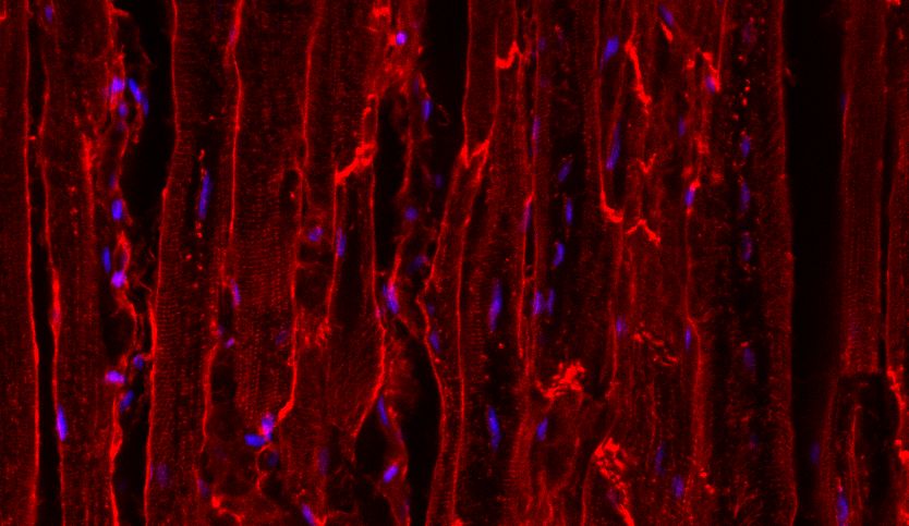
limit on the maximum time step permitted in the random walk, which may pose numerical challenges when long diffusion
times are considered or a large parameter space is to be investigated.
    A number of analytical approaches to the problem of diffusion also exist. Data fitting models attempt to compose the
observed DWI signal as a linear combination of analytical shapes like spheres or ellipsoids for which the contribution is
known23 . This allows for the inference of cell sizes from the measured data. Originally developed for impermeable membranes,
this approach was extended by Karger e.al24 to account for exchange between compartments. While these models offer an
easy way to explain macroscopic observations through integral quantities like the diffusion signal, they do not allow for
deeper insights into the diffusion processes themselves. By reducing the problem to 1D, analytical solutions for the diffusion
propagator can be found. This was first suggested by Tanner et al.25 to estimate the DWI signal in a system of equi-spaced
parallel plates. Very recently, Moutal et al.26 presented a semi-analytical method to obtain the particle density distribution
anywhere in a domain with arbitrary barriers.
    In this work, we study 1D diffusion through semi-permeable membranes and show the numerical limitations of the previous
mentioned reference transit model21, 22 . We propose a new model (hybrid model) based on treating the membrane interface and
the diffusivity discontinuity as two separate probabilities. We analyse the behaviour of both transit model by comparing the
fluxes through the membrane with a semi-analytical solution. A parameter study reveals the errors in the numerical results
and demonstrates that the hybrid model limitations are numerically far less restrictive. Finally, we quantify the impact of our
findings by calculating the difference in DWI signal obtained using both transit model on a realistic histology-based domain
with a wide range of permeability values. This allows us to assess and compare the suitability of both models on diffusion
tensor cardiovascular magnetic resonance (DT-CMR) and to other potential applications.

2 Methods
We describe a method to find (semi-)analytical solutions of the diffusion equation
                                               ∂U(x,t)         h             i
                                                        = ∇ · D(x)∇U(x,t)                                                     (1)
                                                  ∂t
in 1D layered media, i.e. U̇ = ∂∂x [D∂U/∂ x] with piece-wise constant diffusion coefficient D(x).
    In this work, we consider domains as arrays of compartments with constant properties. Figure 1 provides an example
of one such arbitrary domain and explains the nomenclature. The figure also shows cardiomyocytes obtained via confocal
microscopy imaging, typically employed to get detailed structural information about the tissue microstructure. Image data like
this often informs (computational) models of diffusion in biological tissue and aids the inference of tissue properties required
from DWI. Considering that, for typical diffusion length scales, diffusion in the vertical/longitudinal direction (parallel to
the cardiomyocytes) is much less restricted than in the perpendicular direction, the problem may be reduced to 2D for many
applications. Even 1D simulations provide new insights, especially in studying the effect of permeability.
    All parameters uniquely defining the problem (compartment barrier locations bk and corresponding sizes Lk , diffusivities Dk ,
barrier permeabilities κk ) can be arbitrarily chosen, which allows us to consider histology based domains. The choice Dk
permits the modelling of different compartments as intra-cellular (ICS) or extra-cellular space (ECS, which may be interstitial
or intravascular). Even though, at the molecular level, walkers experience the same self-diffusion1 , a mesoscopic model
of a reduced bulk diffusivity accounts for apparent hindrance due to intra-compartmental tissue characteristics. Interfaces
like membranes or intercalated discs may either be modelled with reduced D and small L, or as barriers with appropriate
permeability κ. We set a zero-flux Neumann boundary condition (∇U = 0) for this investigation as walkers do not vanish in
biological tissue.

2.1 Random walk transit models for permeable membranes
The solution to the diffusion equation (1) may be obtained by considering an ensemble of massless, non-interacting particles
performing a random walk. U(x) denotes the probability of a particle being located at a given position. Below, we describe the
random walk process for a single particle/walker, which is repeated N p times per experiment.
2.1.1 A single random walker
We consider a walker with subscript p. At each time step δt, its position x p is updated through a series of sub-steps δ xn that
depend on the local environment:
                                               x p (t + δt) = x p (t) + ∑ δ xn .                                             (2)
                                                                                         n
At the beginning of a time step, a random step vector δ√x is drawn with equal probability of moving in direction +x or −x.
For diffusion away from barriers, a single step δ x = ± 2Dδt is performed. Interaction with barriers introduces additional
  1 The   diffusion coefficient of a given fluid is only dependent on the temperature.

                                                                                                                             2/22
Figure 1. a) Left: Confocal fluorescence microscopy image of cardiomyocytes running vertically. The mean diffusion
distance ∆x ≈ 30 µm over 100 ms is indicated as the radius of the yellow circle. Right: Schematic of an example domain with
m = 4 compartments with indices k. Each compartment has two barriers with their corresponding locations bk , diffusivites Dk ,
and permeabilities κ j . Note that the domain ends enforce the zero-flux boundary conditions (κ0 = κm = 0). b) Illustration of
the behaviour of a single walker at x p performing a random step δ x towards a barrier at xb . Initially, the step is divided into δ xi
and δ x j . Depending on the transit decision, the walker is either reflected elastically (x = x p + δ xi − δ x j ) or enters the new
compartment with D j < Di . In the latter case, the remaining step after transit is modified to δ x0j following equation (3) such
that entering a compartment with lower/higher diffusivity decreases/increases δ x j .
sub-steps, however in this work we consider
a maximum of a single barrier crossing per time step. This imposes a limit on the
Lk
possible time steps, namely δt < mink 2D .
k
If a walker attempts to cross from compartment i to compartment j through a barrier at xb , the step is divided into δ x =
δ xi + δ x j such that δ xi = xb − x p . This is illustrated in figure 1. The interaction is resolved by first computing a probability of
transit pt and then drawing a random number U ∈ [0, 1) to compare to pt . Transit occurs if U < pt , otherwise the walker is
reflected elastically. Upon entering a new compartment with different diffusivity D j 6= Di , the remaining step length δ x j over
δxj
the duration δt j = δ x δt needs to be adjusted to preserve a constant net step size20 :
r
Dj
δ x0j = δ x j (3)
Di
In addition to the above step modification, another condition needs to be satisfied. The probabilities of crossing from either
side to the other, i.e. pt,(i→ j) and pt,( j→i) , must be related by
r
pt,(i→ j) Dj
= . (4)
pt,( j→i) Di
This “interface reflection” is required even as κ → ∞20 .
3/222.1.2 Hybrid model
A number of "transit models" have been proposed to calculate the probability of transit pt based on properties of the membrane
and tissue. The ultimate aim of any such model is to accurately represent the leather boundary condition equation (5)19, 25 .
∂U
Di = κi, j (U|R − U|L ) (5)
∂x L
Here, U is the particle density and the evaluation limits L and R indicate that the concentration and its gradient should be
evaluated infinitesimally to the left (on the side of compartment i) or right (compartment j) of the interface. Fick’s first law27
states that the flux J is related to the gradient in concentration by J = −D∇U, where the sign indicates the direction of the flux
vector with magnitude J. Since there is no accumulation of concentration/walkers inside the barrier, the flux must remain the
same on either side, i.e.
∂U ∂U
Di = Dj . (6)
∂x L ∂x R
The case of a finite membrane permeability with constant diffusivity values (i.e. Di = D j ) is well-studied on a discrete
lattice of equidistant points19 . A recent transit model21, 22 (reference model) extended this approach to particles located at
arbitrary positions x p in the vicinity of the membrane. By neglecting higher-order terms in the derivation and still considering
constant diffusivity (compare appendix A), it is possible to derive a transit probability pt that works for different diffusivites
provided that the time step is small enough such that pt
1 < 0.0121 .
2κi, j δ xi
pt,(i→ j) = , (7)
Di + 2κi, j δ xi
where δ xi is the distance from x p to the barrier xb . With the motivation of lifting this step restriction, we propose a new transit
model (hybrid model) based on treating the diffusivity gradient and the membrane permeability as two independent factors.
This new transit model considers an infinitesimal space between the membrane and the diffusivity change such that the overall
probability can be computed as the product of these two.
pt,(i→ j) = pm,(i→ j) · pd,(i→ j) (8)
Where pm and pd are the membrane probability considering constant diffusivity and the probability of a particle when
transitioning between two different media. The probability pd is presented as an elegant interpretation of the behaviour of
random walkers when transitioning between media of different viscosities.28 .
r !
Dj
pd,(i→ j) = min 1, , (9)
Di
Substituting pm and pd with equation (9) and equation (7) we obtain the overall probability of the new transit model. As
observed in figure 2, this hybrid model presents two possible configurations depending on the location of pm . The first and
second option place the membrane in the low and high diffusivity region respectively. We observe that positioning pm in the
"fast" side (high diffusivity) leads to infinite reflections in between the two membranes (δ s). The model considers δ s → 0
because considering a small δ s would set a high step size restriction. Due to the fact that there is no physical compartment
and infinite reflections when placing pm in the "fast side", the model is only valid when the membrane pm is placed in the
"slow side" (low diffusivity region). Even though locating pm in the fast side is not feasible when δ s → 0, in appendix B, we
mathematically show and validate that the infinite reflections that occur when placing the pm in the high diffusivity region ("fast
side") lead to the same overall probability as placing the membrane pm in the slow slide.
2.2 Flux analysis
We investigate the transient and steady state behaviour of U(x,t; x0 ) in a very simple representative domain using the reference
and new hybrid transit models mentioned in section 2.1.2. We compare the fluxes through the permeable barrier to an analytical
solution. Analysing the fluxes offers more insights into the exchange process, which is modelled as a random process, than
looking at concentrations on either side of the interface. The flux as an integral quantity can be compared easily with the
analytical solution and does not rely on histogram binning, which is prone to noise.
4/22Figure 2. Illustration of the two different configurations depending on where the interface membrane (pm ) is placed.
Configurations 1 and 2 place the membrane in the "slow side" (low diffusivity region) and "fast side" (high diffusivity region)
respectively.
2.2.1 Simple domain
Very few estimates exist in literature for the free diffusivity in the myocardium and/or the permeability of the cardiomyocyte
membrane. A recent study29 observed diffusivity values of 1.2 µm2 /ms and 3 µm2 /ms in the intra- and extra-cellular space of
heart rat cells. A recent numerical study16 performed simulations of a histology-based domain for a range of diffusivities and
found apparent diffusion coefficients (ADC) similar to what is commonly observed in-vivo. The values for DECS had a range
of 1 to 3 µm2 /ms, with DICS varying between 1 µm2 /ms and DECS . In general it should be expected that the compartment-
specific bulk diffusivity are lower than the free diffusivity of water and DICS < DECS due to the concentration of sub-cellular
structures.The cell membrane permeability may be estimated from measurements of apparent exchange rate (1/τex ). The
exchange time constant τex is related to the cell membrane permeability via τex = α (V /S)/κ, where α is the extra-cellular
volume fraction (ECV) and V and S the volume and surface area of the cell respectively. Exchange rates are commonly reported
in a range of 6 to 30 Hz29, 30 , but have been found as high as 50 Hz for healthy leg muscles of rats31 .
We consider a domain with a single permeable barrier separating two compartments of different diffusivities, DL and DR ,
representing intra- and extra-cellular space respectively. This allows us to isolate a single interface and avoid confounding
effects from other compartments. The parameter choice aims to be representative of cardiac tissue. We use DL = 0.5 µm2 /ms
and DR = 2.5 µm2 /ms as compartment diffusivities expected in intra- and extra-cellular space. The membrane permeability is
set to κ = 0.05 µm/ms based on an estimated τex −1 = 30 Hz. The compartment lengths are considered to be equal in both sides
L = 20 µm
2.2.2 Analytical Solution
In order to compare the performance of both transit models we have the necessity to obtain an analytical solution. A recent
study26 presented an elegant transcendental equation F(λ ) := 0 that is to be solved in order to obtain the eigenvalues λ of the
diffusion operator. The eigenvalues are the roots of F(λ ? ) where λ ? is an auxiliary variable considered when F is evaluated on
a continuous range. The solution assumes the time and space variables in equation (1) are separable, resulting in the ansatz
U(x,t) = u(x)e−λt . (10)
For piecewise-constant Dk , the eigenvalue problem is reduced to a Helmholtz equation
Dk u00 + λ u = 0 ∀x ∈ [bk , bk+1 ] . (11)
Using the general solution to this ODE, which is a function of the eigenvalues, one can construct a transcendental equation
ensuring that all boundary conditions are satisfied simultaneously. This is achieved through a series of matrix multiplications
5/22that link compartments together26 . The problem of finding eigenvalues is therefore reduced to that of finding the roots of that
transcendental equation
!
m−2
p 1
√
F(λ ) := κm / λ Dm−1 1 Rm−1 (λ ) ∏ M k,k+1 (λ )Rk (λ ) =0 (12)
k=0
κ0 / λ D0
with auxiliary matrices p p
cos(Lk pλ /Dk ) sin(Lk pλ /Dk )
Rk (λ ) = , (13a)
− sin(Lk λ /Dk ) cos(Lk λ /Dk )
p
1 λ D k /κk,k+1
M k,k+1 (λ ) = p . (13b)
0 Dk /Dk+1
For a sensible choice of permeabilities for internal barriers (0 < κk < ∞, i.e. no trivial cases), there exist a countably infinite
number of real eigenvalues, all of which are non-negative, ordered, and simple26 :
0 ≤ λ1 < λ2 < . . . , λn → ∞ (14)
The eigenvalues of higher order have diminishing importance with increasing solution time t. For the domains in this work,
we use a truncation point of the order of n ≤ O(103 ). The solution is then computed by evaluating and summing the
eigenmodes νi (x) throughout the domain at several linearly-spaced points xq ∈ [0, bm ].
N
U(xq ,t) ≈ ∑ e−λnt νn (xq )νn (xq,0 ) (15)
n=1
The initial condition is always given by a delta Dirac function:
U(xq , 0) = δ (xq − xq,0 ) (16)
As described above, the eigenvalues (roots of equation (12)) are found numerically up to λmax . The solution U(xq ,t) is,
therefore, semi-analytical. As a consequence, numerical errors introduced by the root finding procedure manifest themselves as
errors in the solution. In our simple and complex domains, λmax = 1000 has been observed to be enough for an accurate and
smooth solution. Due to the linearity of the diffusion equation, a uniform initial condition in a certain domain region can be
solved by adding and normalising all the solutions obtained by several delta Dirac functions within the interested interval.
2.2.3 Transient and steady state analysis
We analyse the flux of particles crossing the membranes that is represented from the flux boundary condition in Equation (5).
This equation relates the flux J with the permeability and the difference between concentrations across the barrier. The units
of J are concentration (fraction of walkers) per unit time and area, but we omit the latter such that [J] = 1/ms. This flux
boundary condition, allows us to compute the instantaneous analytical flux evaluating U on either side of the discontinuity and
the instantaneous numerical flux by measuring the fraction of particles that cross the barrier for the each specific time step. The
net instantaneous flux is obtained each time step by subtracting the fluxes from either side (left/right) and the cumulative flux
(flux integral) throughout the simulation.
Based on the analytical and numerical flux comparison, we perform two different types of analysis to evaluate the efficacy
of the transit models. We implement a steady and transient state analysis by considering different initial conditions. A uniform
concentration throughout the domain is considered for the steady-state and a partial uniform distribution for the transient state.
We determine the relative error εglobal for both transit models using the cumulative flux J (t) = 0t J(τ) dτ which represents
R
the net concentration of walkers that has crossed the membrane up until t and approaches 0.5 as t → ∞ to match the steady state
solution. This global relative error εglobal measures the area in between the analytical and numerical solution during the entire
simulation.We utilise this global relative error to investigate the time step dependence and compare the performances of our
new hybrid model and the reference model21 under the influence of different permeability and diffusivity values.
2.3 Diffusion Weighted Imaging (DWI)
2.3.1 Synthesised histology-based domain
The domain has been obtained from sections of swine myocardium, cut perpendicular to the long axis of the cardiomyocytes.
We have used automatic segmentation developed in previous work32 to obtain a distribution of cell sizes. We have utilised
this previous work to find statistics parameters (mean cross-sectional area, standard deviation) to recreate a synthesised
histology-based domain assuming a circular cross-sections for cardiomyocytes33 . The cell areas are converted to diameters
which we use as intra-cellular compartment lenghts in the 1D domain. The extracellular space is recreated considering a
uniform distribution.
6/222.3.2 Random walk simulations in the histology-based domain
For the histology domain simulations, we use N p = 106 walkers and a time step of δt = 1.5 ms as it has been observed to be
enough to converge to an accurate solution. These parameters intentionally exceed the small time step required for accurate
handling of transit using the model in equation (7), while still limiting walkers to a single barrier interaction per step (since
min(LECS ) ≥ 2 µm and DECS = 0.5 µm2 /ms). Random walk simulations are run for t = 1000 ms and the analytical solution is
evaluated for the same space and time parameters. We use the semi-analytical solution described in section 2.2.2 to obtain
1000 eigenvalues with λ ? ∈ [0, 500]. Conversely to section 3.2, the transient solution U(x,t; x0 ) is obtained by seeding all
the walkers at the centre of the domain, while the steady-state solution is initialised by seeding the walkers uniformly. We
use DICS = 0.5 µm2 /ms and DECS = 2.0 µm2 /ms and we set the permeability to κ = 0.05 µm/ms for all cell membranes.
2.3.3 DWI and other potential applications
One important application of Monte Carlo random walk simulations in complex domains is in understanding diffusion weighted
imaging (DWI). We perform numerical simulations of DWI in the histology-based domain using the reference model21, 22 and
our new transit model proposed in section 2.1.2. In DWI, radio-frequency pulses are used to excite hydrogen spins and magnetic
field gradients change their precession according to their gyromagnetic ratio γ = 267.5 × 10⁶ rad/(s T). Each spin/walker p
collects precessional phase Z t
φ p (t) = γ G(τ)x p (τ) dτ (17)
0
during the random walk, subject to two symmetric gradients of strength G and duration δ . At readout/time of echo, the resulting
signal S is the Fourier transform of the medium average diffusion propagator and the signal magnitude is thus related to the
distances that the spins have diffused during time ∆.
The analytical and random walk methods presented previously allow us to solve for the diffusion propagator. By means of
the narrow pulse approximation (NPA)34, 35 it is possible to estimate the DWI signal directly. This assumes that the gradients are
applied instantaneously, i.e. δ → 0 as the wave number q(t) = γ 0t G(τ) dτ remains finite (= γGδ ). In DWI, the strength and
R
timing of the gradients is reflected through a parameter called b-value. In the case of NPA, the b-value is calculated as b = q2 ∆
We seed the walkers uniformly in the histology-based domain and we let them diffuse for a period of 1 second. We analyse
and compare the signal attenuation and apparent diffusion coefficient (ADC) with analytical results for a large time step of
dt = 1.5 ms and a small time step dt = 0.01 ms. In order to provide insights in other potential applications, we consider a wide
range of permeabilities (0 to 1 µm/ms) apart from the biological ambit. We have considered a b-value of 1 ms/µm2 for all the
simulations. Due to the narrow pulse approximation (NPA), the random walk and analytical signal (Srw , Sana ) can be directly
computed using the following equations:
Np
1
Srw (∆, q) =
Np ∑ e−ı q (x p (∆)−x p (0)) (18)
p
2
1
Z
Sana (∆, q) = ∑ e−λn ∆
∑k Lk n Ω
νn (x)eıqx dx (19)
√
Here, ı denotes the imaginary unit −1. The analytical diffusion signal is calculated using an expression derived for
uniform initial seeding26 . In equation (19), we approximate the integral numerically using trapezoidal integration over the
finely-discretised domain. Finally, the apparent diffusion coefficient (ADC) is derived from the signal attenuation through
ADC = − ln(S/S0 )/b (assuming S0 = 1).
3 Results
3.1 Analysis of the steady-state
We use histograms to illustrate the random walk solution, density-normalised such that ρbin = cbin /N p /wbin where cbin and wbin
are the bin count and width respectively. We investigate the time step dependence of the membrane transit model for the simple
domain described in section 2.2.1. Figure 3 shows random walk solutions using the new hybrid model and the reference transit
model21 . We examine different time steps δt (20, 10, 5, 2, 0.5, and 0.05 ms) and two solution times 20 and 1000 ms. For
the short time solution, the reference transit model fails to preserve the initial steady-state solution near the barrier. As the
time increases, a concentration imbalance develops across the barrier. The difference in compartment density ∆U across the
membrane increases with δt and appears to stabilise at some value as t → ∞: For δt = 0.05 ms, the reference model shows
an excess of concentration in the left compartment of 0.88 %, for δt = 20 ms this increases to 10.2 %. In appendix C, we
mathematically prove the reference model limitations. On the other hand, the new hybrid model represents the expected solution
with a constant U with a maximum of ∆U = 0.18 % between all values of t and δt, suggesting that there is no accumulation
7/22T = 20 ms T = 1000 ms
0.028
0.027
0.026
U(x)
0.025
0.024
0.023 Reference model with time step δt:
dt=20.0 ms dt=2.0 ms
0.022 dt=10.0 ms dt=0.5 ms
dt=5.0 ms dt=0.05 ms
0.021
0.028
0.027
0.026
U(x)
0.025
0.024
0.023 Hybrid model with time step δt:
dt=20.0 ms dt=2.0 ms
0.022 dt=10.0 ms dt=0.5 ms
dt=5.0 ms dt=0.05 ms
0.021
0 5 10 15 20 25 30 35 40 0 5 10 15 20 25 30 35 40
x (µm) x (µm)
Figure 3. Histograms of walker positions after random walk simulations of the steady state. Initial positions were sampled
from a uniform distribution to seed walkers with a constant density throughout the domain. We applied the reference membrane
model (Top) described in equation (7), with permeability κ = 0.05 µm/ms, and the new hybrid model (Bottom) from
equation (8). Simulations were performed with varying step sizes δt for a short and a long simulation time t.
of walkers for any time step. The variation in bin densities for the interface model can be attributed to randomness of the
∗ = 1/ L = 0.025 has a
simulation. At t = 1000 ms the difference between observed ρbin values relative to the expected ρbin ∑
∗
median (among δt) standard deviation of 0.0013 (or 5 % relative to ρbin ).
3.2 Analysis of the transient-state
We perform two different transient-state analyses to independently investigate the influence of the step size and the influence of
several permeability and diffusivity values.
3.2.1 The influence of step size
Simulations are performed up to t = 1000 ms using the largest time step (δt = 20 ms) utilised in section 3.1 and small time
step of δt = 0.5 ms. Figure 4 shows the instantaneous and cumulative fluxes obtained from the random walk simulation at
every time step alongside the analytical solution. For the random walk solution, we also plot a time-averaged flux over fixed
intervals of ∆t = 20 ms to allow for comparison between both plots. Note that the time-average flux and instantaneous flux
coincide for the largest time step. The (analytical) flux J rapidly increases early in the simulation and peaks at t = 58.53 ms.
As t increases, walkers continue to cross the membrane towards the initially empty compartment (J > 0 always). We observe
that for a large time step δt = 20 ms , the time-averaged/instantaneous flux for both transit models over-estimate the initial peak
in magnitude. However, if we compare the cumulative fluxes at the final end-point of the simulation (t = 1000 ms, the reference
model underestimates the tail with a relative error of −10.27% compared to an error of −1.87% for the hybrid model. We
observe that reducing the time step increases the number of walkers crossing the membrane increasing the overall convergence.
For δt = 0.5 ms, the relative error at the end of the simulation is reduced to −2.6% and to −0.46% for the reference and hybrid
model respectively. This is consistent with the results observed in figure 3 for the steady-state analysis.
8/22δt = 20 ms δt = 0.5 ms
Inst. Flux (Hybrid Model)
0.0015 Inst. Flux (Ref Model)
20ms Time-average (Hybrid Model)
20ms Time-average (Ref Model)
J (ms−1 )
0.0010
0.0005
0.0000
0.4
J(τ ) dτ
0.3
Rt
0
0.2
J (t) =
0.1 Cumulative Flux (Hybrid Model)
Cumulative Flux (Ref Model)
Analytical Solution
0.0
0 200 400 600 800 1000 0 200 400 600 800 1000
t (ms) t (ms)
Figure 4. Top figures: Instantaneous and time-averaged (plotted as the average of every interval with ∆t = 20 ms) fluxes J(t)
through the membrane as a function of simulation time. Bottom figure: Analytical and numerical net cumulative flux. We show
results for two different step sizes δt: 20 and 0.5 ms. Domain and simulation parameters: DL = 0.5 µm2 /ms,
DR = 2.5 µm2 /ms, κ = 0.05 µm/ms, L = 20 µm, N p = 106 .
3.2.2 The influence of permeability and diffusivity
In order to study the effects of permeability and diffusivity, we consider the simple domain varying the ratio (b = DR /DL )
between diffusivities in either side. We consider a constant left diffusivity of DL = 2 µm2 /ms and a range of ratios (0.05 < b <
2.5). We consider two permeability values (0.05 and 0.5 µm/ms) that correspond to exchange times of the order of 50Hz and
500Hz respectively. The first permeability (0.05 µm/ms) is linked to exchange times that are closer to what we would observe
in human cells29 and the second permeability value covers higher exchange rates that might be useful for other applications.
We perform simulations up to t = 1000 ms for six different time steps δt: 8, 4, 2, 0.5, 0.1, and 0.05 ms and 9 different varying
diffusivity ratios 2.5, 1.8, 1.6, 1, 0.4, 0.2, 0.1, and 0.05 Figure 5 shows the global relative errors that have been computed
by evaluating the integral difference between the numerical and analytical cumulative flux. The top plots and the bottom
plots illustrate the global errors for the reference model and hybrid model respectively. As mentioned in section 2.2.3, each
simulation has been performed initialising the walkers in a partial uniform region within the left compartment. For a constant
permeability, we observe that the global errors escalate as we increase the difference between diffusivities. These increments
are consistently lower for the hybrid model as it includes the probability when transitioning between two different media
through equation (9). Similarly to figure 4, lowering the step size increases the number of walker collisions with the membrane
resulting in an overall faster convergence and accuracy. As it can be observed in equation (8), the hybrid model incorporates
the reference model to solve the membrane/interface probability. In appendix C.3, we show that the reference model does not
preserve the interface reflection and leads to a permeability-related error. As a result, both models show a permeability error
dependency, however, the hybrid model relative errors are consistently lower due to the initial error reduction in the diffusion
media.
9/22κ = 0.05 µm ms−1 κ = 0.5 µm ms−1
10 12
0.05 2.4 3.7 9 13 23 29 16 23 43 52 69 74
Ref. Model - (DR : DL ) 0.1 1.4 2.2 5.4 7.3 14 17 10 15 27 33 45 49 10
8
0.2 0.71 1.1 2.8 3.7 7.3 9.1 5.3 7.8 15 19 26 29
global (%)
global (%)
8
0.4 0.26 0.45 1.3 1.6 3.2 4.1 6 2 3.2 6.9 8.7 13 14
6
1 0.11 0.12 0.1 0.16 0.16 0.72 1 0.95 0.92 1 0.98 1.5
4
1.6 0.28 0.25 0.48 0.77 1.3 2.3 2.1 2.6 4.1 5 6.7 8.2 4
1.8 0.21 0.26 0.55 0.97 1.6 2.6 2 2.4 2.9 4.8 5.9 8.2 9.7 2
2.5 0.24 0.4 0.79 1.2 2.2 3.4 3 3.9 6.5 8.2 12 14
0 0
10 12
0.05 1.5 1.7 2.3 2.9 4.7 6.7 9.9 10 11 11 13 14
Hybrid Model - (DR : DL )
0.1 0.84 1 1.5 2.1 3.3 5 5.5 5.6 6.2 6.7 8 9.3 10
8
0.2 0.5 0.55 1 1.3 2.1 3.4 3.1 3.2 3.5 3.9 4.7 5.7
global (%)
global (%)
8
0.4 0.19 0.31 0.45 0.72 1.1 2.1 6 1.8 1.8 2 2.2 2.6 3.4
6
1 0.13 0.11 0.15 0.17 0.11 0.78 1 0.96 0.96 1.1 1 1.6
4
1.6 0.16 0.096 0.17 0.29 0.44 1.1 0.79 0.88 0.89 0.99 1.1 1.8 4
1.8 0.15 0.11 0.18 0.38 0.47 1.3 2 0.79 0.82 0.89 0.99 1.2 1.7 2
2.5 0.18 0.2 0.18 0.4 0.65 1.4 0.74 0.8 0.78 0.99 1.2 1.7
0 0
0.05 0.1 0.5 2 4 8 0.05 0.1 0.5 2 4 8
δt(ms) δt(ms)
Figure 5. Errors in the random walk for different time steps δt and permeabilities κ in four different domains (the left-most
domain is the model domain used in sections 3.1 and 3.2). Simulations were run until t = 1000 ms with N p = 106 walkers
seeded at x0 = 10 µm. Top: The global error (relative to Jana dt) quantifies the degree to which the solution fluctuates around
R
the analytical solution during the simulation. Bottom: The cumulative error (relative to Jana ) represents the error in net flux at
the end of the simulation.
3.3 Transient and steady-state solutions in the histology-based domain
Figure 6 illustrates the distribution of cell sizes for the manual and automatic segmentation32 . As explained in section 2.3.1, we
recreate a histology-based domain by considering circular cross-sections for cardiomyocytes. The segmentation data shows
a mean cross-sectional area of µ = 120 µm2 and a standard deviation of σ = 40 µm2 . We utilise these parameters to create a
synthesised histology-based domain using a normal distribution ( µ ± 2σ ) for the intra-cellular space and a uniform distribution
(3 µm-5 µm) for the extra-cellular compartments. The resulting domain is recreated by drawing both intra-cellular and extra-
cellular distributions until reaching a total length of 49.5 µm. Figure 7 shows the final steady state and three different transient
states for the histology-based domain. The transient states are analysed at three different diffusion times T = 50, 100, 1000ms
considering that all the particles are initialised in the middle of the domain X0 = 24.75 µm. We observe good agreement between
the hybrid model and the analytical solutions. We notice that the reference model tends to be less restrictive in the initial
transient states leading to higher concentrations in the ECS. This accumulation of walkers is present and is carried during the
entire simulation until reaching the steady-state. This excess of walkers in the ECS persists throughout the simulation and is
consistent with the findings in section 3.1 and section 3.2.
3.4 DWI results
We analyse how the diffusion errors observed in section 3.3 affect the DWI signal and apparent diffusion coefficient (ADC).
We compare the signal attenuation and ADC with the theoretical analytical results. As mentioned in section 2.3.3, we seed
the walkers uniformly and consider the narrow pulse approximation (NPA). Figure 8 shows the ADC and the absolute signal
relative error for a large interval of membrane permeabilities and two different step sizes. Equation (18) shows the relation
between the numerical signal error and the displacement of the walkers. Similarly to the flux analysis, we notice a strong
dependency between the permeability and the accuracy of both transit models. If we compare the errors for different increasing
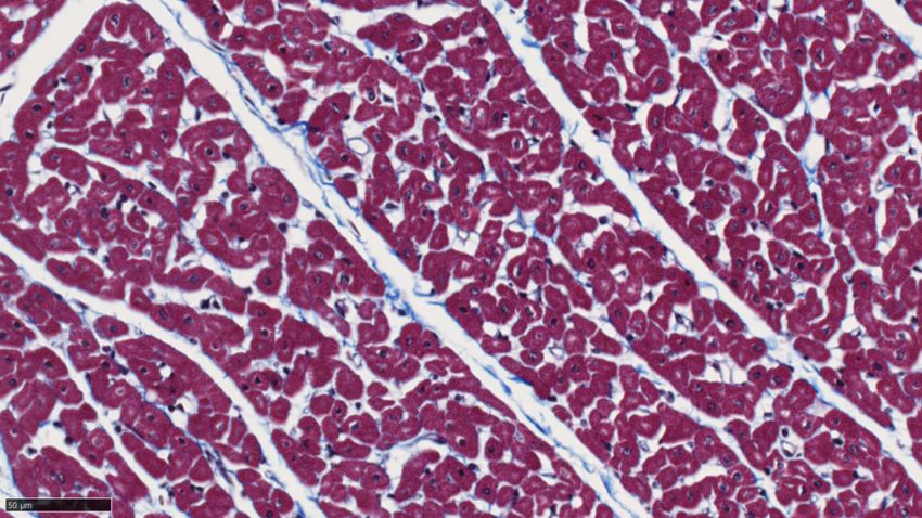
10/22Example histology image Estimated myocyte size
0
0.200
Area = 120 µm2
Segmentation (automatic)
0.175
Segmentation (manual)
0.150
0.125
Height (µm)
probability
0.100
0.075
0.050
0.025
0.000
244
0 434 0 100 200 300 400 500 600
Width (µm) Area (µm2 )
Compartments of synthesised domain
Figure 6. Illustration
Membrane ICS of theECSprocess of synthesising a 1D domain from histology data. Left Figure: An example of a region of
histology from a wide-field microscopy image. This is part of a large vertical stack of histological slices obtained from the
mesocardium of swine. Cardiomyocytes (red-purple) are cut perpendicular to the imaging plane. Extra-cellular space is white,
while collagen is stained blue. Right Figure: Distribution of cell sizes from automatic segmentation for the entire stack of
0 6 23 38 50 65 80 94 108 121 136 153 168 183 201 216 230 246 262 278 291 296
images as well as manual labelling of a small representativexregion.
(µm)
permeability values, we observe that the reference model progressively becomes less accurate. We initially report low relative
errors (≈ 0.3%) for δt = 1.5ms that scale up to 0.8% for the reference model. These signal and ADC errors can be reduced
when decreasing δt due to the increment of particle collisions against the membranes. In the application that we are interested
in, the cardiomyocytes have low permeability values (κ < 0.05µm/ms)31 where both transit models perform similarly with low
relative errors.
11/22T = 50 ms T = 100 ms T = 1000 ms
0.06 0.06 0.06
0.04 0.04 0.04
U(x)
0.02 0.02 0.02
0.00 0.00 0.00
0 10 20 30 40 50 0 10 20 30 40 50 0 10 20 30 40 50
Length (µm) Length (µm) Length (µm)
Steady State
0.0250 Analytical Solution
Hybrid model
0.0225 Ref Model
U(x)
0.0200
0.0175
0.0150
0 10 20 30 40 50
Length (µm)
Figure 7. Analytical and random walk solutions (using N p = 106 walkers and a time step of δt = 1.5 ms) at t = 1000 ms. Top:
Transient solution U(x,t; x0 ) for initial concentration at x0 located in the centre of the domain. Bottom: Steady-state solution
after uniform seeding of walkers in the domain. The reference model results in accumulation of walkers in ECS compartments.
Note that this effect is visually amplified by the choice of axis data range.
0.22
Apparent Diffusivity Coefficient (ADC) µm2 ms−1
0.8
Absolute Signal Relative Error (%)
0.20 0.7
0.6
0.18
0.5
0.16
0.4
0.15
0.125 0.3
Hybrid Model δt = 0.01ms
0.1 Ref Model δt = 0.01ms 0.2
0.075 Hybrid Model δt = 1.50ms
0.05 Ref Model δt = 1.50ms 0.1
0.025 Analytical ADC Values
0.0
0
0 0.05 0.2 0.4 0.6 0.8 1 0 0.2 0.4 0.6 0.8 1
−1 −1
Permeability κ (µm ms ) Permeability κ (µm ms )
Figure 8. Absolute relative signal error and ADC values for a wide range of permeability values considering a very small
(δt = 0.01 ms) and large time step (δt = 1.5 ms). All the simulations consider N p = 106 walkers, DECS = 2 µm2 /ms and
DICS = 0.5 µm2 /ms
12/224 Discussion
Simulating the transit of particles through a semi-permeable membrane separating media with differing diffusivities can be
achieved using analytical or numerical techniques. In this work, we present novel methods for determining the particle density
in a 1D domain and the flux through a membrane.
Monte Carlo random walk based method are frequently used to solve the diffusion equation (1) in a range of applications.
When a walker encounters a barrier such as a semi-permeable membrane, the probability of transit needs to be accurately
computed and the walker step size must be adjusted to satisfy equation (3) when transiting between compartments of differing
diffusivities20 . One of these so-called transit models is the popular method described in equation (7)21 . As described in the
original paper, this reference transit model21 requires a highly resolved time step. For this reason, it is suggested that the
maximum time step (δtmax ) is limited by a maximum possible transmission probability of 0.0121 . This can be a computational
challenge for long and even short diffusion time simulations when other Monte Carlo parameters such as the number of
walkers N p or the number of unique experiments need to be considered. In this work we propose a new hybrid transit model with
the motivation of lifting this restriction. The new model that we present is based on treating the membrane as an infinitesimal
space such that the diffusivity gradient and the membrane permeability can be considered as two independent factors. It is
important to note that the hybrid model is built on top of the reference model as it is used to solve the membrane probability.
Using an analytical solution as a gold standard, we have studied the accuracy of the hybrid and reference transit model21 when
exceeding the maximum step size (δtmax ). We have assessed both models by analysing the membrane flux varying several
parameters in a simple geometry domain.
We have found that the reference model leads to errors in the net migration of walkers and results in concentration
imbalances for steady-state solutions. Further analysis in appendix C demonstrated that the transit model inherently tends to
accumulate walkers when the membrane divides two compartments of different diffusivities. In appendix C.3 we also note that
the interface reflection condition in equation (4) is not respected as κ → ∞ and this is consistent with the findings observed
for both transit models in figure 5 and with the relation between diffusivity/permeability to fit within the maximum time step
(δtmax ).
The numerical simulations performed in this study consider a fixed step size. In Section 3.2, we have considered a partial
uniform distribution of walkers in the left compartment to avoid sampling error for large step sizes due to the unique number
of possible walker positions. From the numerical simulations in the simple domain, we numerically prove the limitations of
the reference model for varying diffusivities. From our steady-state and transient findings, we conclude that these imbalances
increase for higher step sizes and longer diffusion times. Further numerical analysis shows that the hybrid model substantially
reduces the diffusivity and permeability-related errors present in the reference model. It is important to note that when there is
no diffusivity discontinuity the hybrid model is in pure essence the reference model itself. Our results demonstrate that the
hybrid model successfully lifts the time step restriction and other numerical limitations.
One important application of the methods presented in this work is in the simulation of diffusion weighted imaging (DWI).
Previous numerical simulations of diffusion tensor imaging (a variant of DWI) in the heart were based on impermeable
membranes16 and resulted in more anisotropic diffusion than commonly found in imaging studies36 . Initial work using finite
volume methods37 has suggested that this underestimation of anisotropy is likely due, at least in part, to the failure to include
permeability within the model.
The simulations in section 3.3 use a domain constructed based on microscopy images of histology sections. Using
a previously developed method32 to automatically segment cells, we have extracted characteristic cell sizes to generate a
representative one-dimensional domain. A mean cell area of 120 µm, which corresponds to a diameter of 12.4 µm assuming
circular cells was obtained from segmentation of the data. This value is slightly lower than the reported range of 17 to 25 µm
in33 . However, tissue is known to shrink during histological preparation and this may be compensated for during image
processing by morphing the domain as shown in16 .
The cardiomyocyte membrane permeability (κ = 0.05 µm/ms) and the diffusivity values (DECS = 2 µm2 /ms, DICS =
0.5 µm2 /ms) in the histology-based simulations limit the dtmax to extremely low values δt ≈ 0.002 ms. Similarly to the simple
domain analysis, our histology-based results for the reference model show accumulation of particles in the ECV that are carried
along the DWI signal computation. We have observed that both models have very small and similar errors for low permeability
in the range of cardiomyocytes. We have shown increasing errors in the results of the reference model with larger permeability
values. The findings regarding the limitations of the reference model at high κ and larger ratios of D between compartments
are particularly important for applications beyond biological tissue such as heat transfer where different sets of parameters
may be required. For example, a thin layer of material in heat conduction problems can be modelled as a membrane with
permeability D/L.
The complex three-dimensional cardiac microstructure is often successfully modelled as being two-dimensional. We have
attempted to reduce it further to a 1D domain to make use of analytical techniques to validate our new hybrid model and
compare the performance with a previously random walk transit model.. This has provided useful insights into the behaviour of
13/22both model for multiple applications. In future work, we plan to extend the thorough validation performed here into higher
dimensions. For example, there exists an analytical solution in 2D using radial coordinates38 and the finite volume method
offers a well-understood reference solution37 . Computationally, the extension of the random walk into higher dimensions
is trivial by considering the boundary-normal distance for the distance δ xi in equation (7) as discussed in21 . The interface
model in equation (9) is valid for any dimension as it relies on the length of the step28 . Yet other methods involving kinetic
approximation39 or a dual-probability-Brownian motion scheme40 warrant further investigation.
5 Conclusions
Modelling diffusion within non-simple layered media requires a correct treatment of the particle transit at membranes when
numerical solutions are employed.
We investigate the accuracy of a previously proposed transit model for varying diffusion coefficients in the presence of
permeable barriers. We compared the numerical results to an analytical method and show the limitation of this reference
transit model. We propose an alternative to this problem by considering a hybrid transit model that treats the transitioning
between different media and the membrane as two separate probabilities. By comparing numerical and analytical simulations,
we conclude that the new transit model performs with lower errors and successfully lifts the step restriction reducing the
accumulation of walkers observed in the reference model. While random walk methods for the solution of the diffusion equation
in layered media have a number of potential applications, we have considered simulating diffusion-weighted imaging in cardiac
tissue.
For the given range of extracellular compartment lengths we find that the time step is already very restricted by the domain
itself as the walkers cannot cross multiple compartments. We conclude that in application to cardiac tissue, both transit models
present very small and similar errors in the apparent diffusion coefficient, an important integral quantity for diffusion-weighted
imaging. However, other applications where the compartment length are larger and both permeabilities and diffusivites are
higher, the potential of this new hybrid model can be fully realised. In these cases, the hybrid model becomes a computationally
more efficient and more accurate alternative for solving the diffusion equation than existing models.
Acknowledgments
Confocal microscopy images were obtained in collaboration with Dr. Padmini Sarathchandra at The Magdi Yacoub Institute,
and the Facility for Imaging by Light Microscopy at Imperial College London. Dr. Sonia Nielles-Vallespin kindly provided the
wide-field microscopy images of histology slices.
Declarations
Author contributions statement
Conceptualization: IA, JR, DJ.D; Formal analysis and investigation: IA, JR; Writing - original draft preparation: IA, JR
; Writing - review and editing: AD.S, DJ.D; Funding acquisition: AD.S, DJ.D ; Supervision: AD.S, DJ.D; Software:IA,JR
Additional information
Funding This work was funded by British Heart Foundation grants RE/13/4/30184 and RG/19/1/34160. Conflict of interest
The authors declare that they have no conflict of interest.
References
1. Hickson, R. I., Barry, S. I. & Mercer, G. N. Critical times in multilayer diffusion. Part 1: Exact solutions. Int. J. Heat Mass
Transf. 52, 5776–5783, DOI: 10.1016/j.ijheatmasstransfer.2009.08.013 (2009).
2. Vignoles, G. L. A hybrid random walk method for the simulation of coupled conduction and linearized radiation
transfer at local scale in porous media with opaque solid phases. Int. J. Heat Mass Transf. 93, 707–719, DOI: 10.1016/j.
ijheatmasstransfer.2015.10.056 (2016).
3. Decamps, M., De Schepper, A. & Goovaerts, M. Applications of δ -function perturbation to the pricing of derivative
securities. Phys. A: Stat. Mech. its Appl. 342, 677–692, DOI: 10.1016/j.physa.2004.05.035 (2004).
4. Berestyki, H. & Rodriguez, N. Analysis of a heterogeneous model for riot dynamics: The effect of censorship of
information. Eur. J. Appl. Math. 27, 554–582, DOI: 10.1017/S0956792515000339 (2016).
5. Zhang, M. Calculation of diffusive shock acceleration of charged particles by skew Brownian motion. The Astrophys. J.
541, 428–435, DOI: 10.1086/309429 (2000).
14/226. Berkowitz, B., Cortis, A., Dentz, M. & Scher, H. Modeling non-Fickian transport in geological formations as a continuous
time random walk. Rev. Geophys. 44, DOI: 10.1029/2005RG000178 (2006).
7. Kärger, J., Ruthven, D. M. & Theodorou, D. N. (eds.) Diffusion in Nanoporous Materials (John Wiley & Sons, 2012).
8. Stejskal, E. O. & Tanner, J. E. Spin diffusion measurements: Spin echoes in the presence of a time-dependent field gradient.
The J. Chem. Phys. 42, 288–292, DOI: 10.1063/1.1695690 (1965).
9. Le Bihan, D. Looking into the functional architecture of the brain with diffusion MRI. Nat. Rev. Neurosci. 4, 469–480,
DOI: 10.1038/nrn1119 (2003).
10. Basser, P. J., James, M. & Le Bihan, D. Estimation of the effective self-diffusion tensor from the NMR spin echo. J. Magn.
Reson. Ser. B 103, 247–254, DOI: 10.1006/jmrb.1994.1037 (1994).
11. Le Bihan, D. & Johansen-Berg, H. Diffusion MRI at 25: Exploring brain tissue structure and function. NeuroImage 61,
324–341, DOI: 10.1016/j.neuroimage.2011.11.006 (2012).
12. Nielles-Vallespin, S. et al. Cardiac diffusion: Technique and practical applications. J. Magn. Reson. Imaging 52, 348–368,
DOI: 10.1002/jmri.26912 (2020).
13. Fieremans, E. & Lee, H.-H. Physical and numerical phantoms for the validation of brain microstructural MRI: A cookbook.
NeuroImage 182, 39–61, DOI: 10.1016/j.neuroimage.2018.06.046 (2018).
14. Yeh, C.-H. et al. Diffusion Microscopist Simulator: A general Monte Carlo simulation system for diffusion magnetic
resonance imaging. PLOS ONE 8, 1–12, DOI: 10.1371/journal.pone.0076626 (2013).
15. Palombo, M., Alexander, D. C. & Zhang, H. A generative model of realistic brain cells with application to numerical
simulation of the diffusion-weighted MR signal. NeuroImage 188, 391–402, DOI: 10.1016/j.neuroimage.2018.12.025
(2019).
16. Rose, J. N. et al. Novel insights into in-vivo diffusion tensor cardiovascular magnetic resonance using computational
modelling and a histology-based virtual microstructure. Magn. Reson. Medicine 81, 2759–2773, DOI: 10.1002/mrm.27561
(2019).
17. Reese, T. G. et al. Imaging myocardial fiber architecture in vivo with magnetic resonance. Magn. Reson. Medicine 34,
786–791, DOI: 10.1002/mrm.1910340603 (1995).
18. Bruvold, M., Seland, J. G., Brurok, H. & Jynge, P. Dynamic water changes in excised rat myocardium assessed by
continuous distribution of T1 and T2. Magn. Reson. Medicine 58, 442–447, DOI: 10.1002/mrm.21340 (2007).
19. Powles, J. G., Mallett, M. J. D., Rickayzen, G. & Evans, W. A. B. Exact analytic solutions for diffusion impeded by an
infinite array of partially permeable barriers. Proc. Royal Soc. A 436, 391–403, DOI: 10.1098/rspa.1992.0025 (1992).
20. Szafer, A., Zhong, J. & Gore, J. C. Theoretical model for water diffusion in tissues. Magn. Reson. Medicine 33, 697–712,
DOI: 10.1002/mrm.1910330516 (1995).
21. Fieremans, E., Novikov, D. S., Jensen, J. H. & Helpern, J. A. Monte Carlo study of a two-compartment exchange model of
diffusion. NMR Biomed. 23, 711–724, DOI: 10.1002/nbm.1577 (2010).
22. Lee, H.-H., Papaioannou, A., Novikov, D. S. & Fieremans, E. In vivo observation and biophysical interpretation of
time-dependent diffusion in human cortical gray matter. NeuroImage 222, DOI: 10.1016/j.neuroimage.2020.117054
(2020).
23. Panagiotaki, E. et al. Compartment models of the diffusion MR signal in brain white matter: A taxonomy and comparison.
NeuroImage 59, 2241–2254, DOI: 10.1016/j.neuroimage.2011.09.081 (2012).
24. Kärger, J. NMR self-diffusion studies in heterogeneous systems. Adv. Colloid Interface Sci. 23, 129–148, DOI: 10.1016/
0001-8686(85)80018-X (1985).
25. Tanner, J. E. Transient diffusion in a system partitioned by permeable barriers. Application to NMR measurements with a
pulsed field gradient. The J. Chem. Phys. 69, 1748–1754, DOI: 10.1063/1.436751 (1978).
26. Moutal, N. & Grebenkov, D. Diffusion across semi-permeable barriers: Spectral properties, efficient computation, and
applications. J. Sci. Comput. 81, 1630–1654, DOI: 10.1007/s10915-019-01055-5 (2019).
27. Fick, A. Ueber Diffusion. Annalen der Physik 170, 59–86, DOI: 10.1002/andp.18551700105 (1855).
28. Maruyama, Y. Random walk to describe diffusion phenomena in three-dimensional discontinuous media: Step-balance
and fictitious-velocity corrections. Phys. Rev. E 96, DOI: 10.1103/PhysRevE.96.032135 (2017).
15/2229. Seland, J. G., Bruvold, M., Brurok, H., Jynge, P. & Krane, J. Analyzing equilibrium water exchange between myocardial
tissue compartments using dynamical two-dimensional correlation experiments combined with manganese-enhanced
relaxography. Magn. Reson. Medicine 58, 674–686, DOI: 10.1002/mrm.21323 (2007).
30. Coelho-Filho, O. R. et al. Quantification of cardiomyocyte hypertrophy by cardiac magnetic resonance: Implications for
early cardiac remodeling. Circulation 128, 1225–1233, DOI: 10.1161/CIRCULATIONAHA.112.000438 (2013).
31. Sobol, W. T., Jackels, S. C., Cothran, R. L. & Hinson, W. H. NMR spin–lattice relaxation in tissues with high concentration
of paramagnetic contrast media: Evaluation of water exchange rates in intact rat muscle. Med. Phys. 18, 243–250, DOI:
10.1118/1.596722 (1991).
32. Rose, J. N. et al. Deep learning based segmentation of cardiomyocytes to aid numerical simulations of diffusion
cardiovascular magnetic resonance. In Proceedings of the ISMRM 26th Annual Meeting & Exhibition, 5238 (International
Society for Magnetic Resonance in Medicine, 2018).
33. Tracy, R. E. & Sander, G. E. Histologically measured cardiomyocyte hypertrophy correlates with body height as strongly
as with body mass index. Cardiol. Res. Pract. 2011, DOI: 10.4061/2011/658958 (2011).
34. Callaghan, P. T. Physics of diffusion. In Jones, D. K. (ed.) Diffusion MRI, chap. 4, DOI: 10.1093/med/9780195369779.003.
0004 (Oxford University Press, 2010).
35. Grebenkov, D. S., Van Nguyen, D. & Li, J.-R. Exploring diffusion across permeable barriers at high gradients. I. Narrow
pulse approximation. J. Magn. Reson. 248, 153–163, DOI: 10.1016/j.jmr.2014.07.013 (2014).
36. von Deuster, C., Stoeck, C. T., Genet, M., Atkinson, D. & Kozerke, S. Spin echo versus stimulated echo diffusion tensor
imaging of the in vivo human heart. Magn. Reson. Medicine 76, 862–872, DOI: 10.1002/mrm.25998 (2016).
37. Rose, J. N., Sliwinski, L., Nielles-Vallespin, S., Scott, A. D. & Doorly, D. J. Studying the effect of membrane permeability
with a GPU-based Bloch–Torrey simulator. In Proceedings of the ISMRM 27th Annual Meeting & Exhibition, 3644
(International Society for Magnetic Resonance in Medicine, 2019).
38. Singh, S., Jain, P. K. & Uddin, R. Analytical solution to transient heat conduction in polar coordinates with multiple layers
in radial direction. Int. J. Therm. Sci. 47, 261–273, DOI: 10.1016/j.ijthermalsci.2007.01.031 (2008).
39. Lejay, A. & Maire, S. Simulating diffusions with piecewise constant coefficients using a kinetic approximation. Comput.
Methods Appl. Mech. Eng. 199, 2014–2023, DOI: 10.1016/j.cma.2010.03.002 (2010).
40. Gong, Z. et al. DEM and dual-probability-Brownian motion scheme for thermal conductivity of multiphase granular
materials with densely packed non-spherical particles and soft interphase networks. Comput. Methods Appl. Mech. Eng.
372, 113372, DOI: 10.1016/j.cma.2020.113372 (2020).
A Reference transit model derivation
The work in19 presents a derivation of the transit probability pt for walker positions on a lattice based on a constant step length
in the entire domain. Here, we consider domains where the diffusivity between compartments may differ and re-derive the
probability of transit for the domain in figure 9 considering the different step lengths.
Consider the probability of finding a walker at x p as the sum of probabilities of neighbouring walkers jumping to x p . Away
from interfaces, this results in
1 1
U(x p ,t + δt) = U(x p − δ x,t) + U(x p + δ x,t) . (20)
2 2
Selecting x p to be near a barrier at xb (see figure 9 for the possible paths of walkers to reach this position) results in additional
terms involving pt (both pt,L→R and pt,R→L ). The barrier location is chosen to coincide with a grid point. A walker located
here will proceed left/right according to the appropriate probability of transit. The contributions of different U(x,t) terms
to U(x p ,t + 2δt) in figure 9 (with the path colour indicated) are:
1 1 1 − pt,L→R pt,R→L
U(x p ,t + 2δt) = U(x p − 2δ xL ,t) + U(x p ,t) + U(x p ,t) + U(x p + δ xL + δ xR ,t) (21)
|4 {z } |4 {z } | 2 {z } | 2 {z }
free diffusion (red) free diffusion (blue) reflection (green) transit (orange)
One may now express x p relative to xb , e.g. the contribution of the orange path from the right side of the barrier is:
U(x p + δ xL + δ xR ,t) = U(xb + δ xR ,t) (22)
16/22You can also read