Ranking Prediction of Premier League Study on Regression Modelling

Ranking Prediction of Premier League

 Study on Regression Modelling

 By
 LAI Cheuk Kwan
 17226791

A thesis submitted in partial fulfillment of the requirements for the degree
 of

 Bachelor of Science (Honours)
 in Mathematics and Statistics

 at

 Hong Kong Baptist University

 Data 4th Dec 2020

Content

1 ABSTRACT 4
2 BACKGROUND INTRODUCTIONS 5
3 METHODOLOGIES – REGRESSION MODEL 6

4 DATA AND MODEL I
 4.1 Data Description 7
 4.2 Variables Description 8
 4.3 Standardization 11
 4.4 Model Description 12

5 MODEL EVALUATIONS I
 5.1 Residual Analysis I 14
 5.2 Coefficient of Determination I 19

6 RESULT OF MODEL I 20

7 MODEL REFORMING
 7.1 Multi-collinearity 22
 7.2 Stepwise regression method 25

8 MODEL EVALUATIONS II
 8.1 Residual Analysis II 27
 8.2 Coefficient of Determination II 29

9 DATA AND MODEL II 30
10 RESULTS OF MODEL II 31
11 COMPARISON OF MODEL I AND II 32

12 PREDICTIONS OF 20/21 SEASON FINAL TABLE 34
13 DISCUSSIONS OF LIMITATIONS 35
14 CONCLUSIONS 37

15 REFERENCE 38

ACKNOWLEDGEMENT

Part of the work presented in this thesis was done in collaboration with my supervisor,
Dr. C.K. Yau, the Lecturer of Department of Mathematics, Hong Kong Baptist
University. Without his guidance and help, the completion of this project would not be
finished.

 Signature of Student

 Student Name

 Department of Mathematics
 Hong Kong Baptist University

 Date:

1 Abstract

This thesis is studying the ranking prediction of Premier League by regression method.
The aim of this thesis is to analyze the key variables that should be considered for the
final ranking table. And to carry out the final ranking prediction of Premier League
2020 – 2021 season.

To begin with, this thesis would focus on developing the regression model of ranking
prediction. This thesis would identify what variables should be considered under a
football league. Then I would test the model and check whether trustful or not.

Secondly, this thesis would focus on improving the accuracy and effectiveness of the
model. This thesis would apply different techniques, i.e. checking collinearity,
normalization, and stepwise method, in order to fit the regression model. After
constructing a new model, this thesis would compare the accuracy of the new model
and original one.

2 Introduction

Premier League (PL)

The Premier League (PL) is the top tier of football pyramid in England and one of the
top five football leagues in Europe because of its popularity, quality of competition, as
well as the football stars and coaches.

Each season starts from mid-August and ends in mid-May. Each football team needs to
battle with every single team twice, once at home, which is their home stadium, and
once playing as an away team in their opponent’s stadium. There are 20 teams
contesting the honor of champion each season. Each team needs to play 38 matches,
and in total, there are 380 matches per season.

The fundamental aspect of each football game, no doubt that, is scoring the goals.
Despite other aspects, such as defending, saving, and possessing, most of the
memorable and impressive moments of each match, is putting the ball into the net.
Three are three results after a match: win, draw, or lose.

In PL, each team would award 3 points for a win, 1 point for a draw and none for a
loss. In the end of the season, the team which has the highest points, would be awarded
the champion. The final point table is ranked in order. If more than 1 clubs receive the
same points, then it would be ranked by the goal difference in order.

At the end of each season, the top 4 teams in the table are qualified to join the UEFA
Champions League (UCL), a world class league involving all the top football clubs from
different leagues in Europe. The 5 – 7 teams have a chance to join the UEFA Europe
 th th

League (UEL), a tier two international league involving different clubs. On the other
hand, PL implements a system called promotion and relegation. It means that 4 teams
on the bottom need to drop down into the tier 2 league in England, called English
Football League Championship (EFL). And the top 4 teams in EFL can be promoted
to PL.

It shows us the importance of predicting the final table that we can determine which
teams can be qualified to join international leagues and which teams are needed to drop
down.

Prediction of Premier League Table

There are many prediction of football games by different methods in the world, that
wanting to predict the result of each game. It is useful for people to bet and gamble.

 Figure 1 – Cap Screen of footballpredictions.com

These predictions want to find out the result of each game by analyzing their
performance. However, for our prediction, we want to find out the final ranking of PL.
It is very useful because it can determine the qualification of international leagues.
Getting a higher ranking in PL and the qualification of international leagues, can earn a
large profit. Joel. O. (2009) mentions that UEFA Champions League (UCL) will pay
clubs between €2 million to €15 million for a fix reward, and up to €40 million for
bonus reward base on the value of market. On the other hand, getting higher ranking in
PL would get more supporters. The supporters of the team will buy the tickets to watch
the game, or buy some souvenirs of the team. It shows us the prediction of the table is
very useful for the financial planning of each team.

Joel. O. (2009) had done a similar regression model to predict the final ranking, with 6
variables, which were % Goals to shot, ratio of short/long pass, etc. The aim of this
thesis is to find a more precise model.

3 Methodology - Regression Analysis

Regression analysis is a set of statistical methods, it is useful for estimation of the
relationship between a dependent (target) variable and a set of independent variables
(predictors). Multiple linear regression method, one of the statistical methods of
regression analysis, is a powerful tool for predicting our dependent variable ( ), by
more than one predictors ( 1 , 2 , … , ).

Suppose we have a data set, the data is obtained as the followings:
 Predictor variable ( 1 , 2 , … , )
 1 11 12 ⋯ 1 
 2 21 22 ⋯ 2 
 ⋮ ⋮
 1 2 ⋯ 
 Table 1 – Simple of Data Set

The multiple linear regression model can be written as
 = 0 + 1 1 + 2 2 + ⋯ + + 

The n-tuples of observations also follow the same model. Like
 1 = 0 + 1 11 + 2 12 + ⋯ + 1 + 1
 2 = 0 + 1 21 + 2 22 + ⋯ + 2 + 2
 ⋮
 = 0 + 1 1 + 2 2 + ⋯ + + 

while 0 , 1 , 2 , … , are a set of unknown parameters, denoted as ( ), which are
the regression coefficients associated with ( 1 , 2 , … , ). We are going to estimate the
parameters ( ) from the dataset.

There are some assumptions of error ( ) are needed in the regression model in order
to draw the statistical inferences, as
 ~ (0, 2 )
and
 , = 0, ≠ 
means the ’s are uncorrelated with 0 covariance.

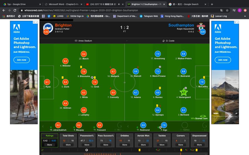
4 Data Description and Setting Up Model

This Chapter will mainly focus on data description and introducing how to construct
the multiple linear regression model. Firstly, this chapter would introduce the source of
data set. Then, it would focus on the predictors we use.

4.1 Data Description

The sources of the data are from www.whoscored.com. As there are no data sets
consisting all the predictors we need, so it is needed to construct myself by recording all
the predictors in every single match we considered individually.

 Figure 2 – Source of one of a Match

The data set what this research use, is consisting 11 seasons, from 09/10 to 19/20 of
Premier League, including the predictors from different football teams which played in
PL. For the construction of the data set, we are going to use the predictors of all teams
in first half seasons, there are 19 matches each team. After that, we would predict the
final points of each team.

Firstly, we would use the data of 09/10 – 17/18, including 9 seasons, to test the model
for 18/19 prediction. Then, we would use 09/10 – 18/19, including 10 seasons to test
for 19/20 prediction. The aims of that is to check whether the regression model is
precise or not.

4.2 Variables Description

For the principle of multiple linear regression, we need a set of independent
variables ( 1 , 2 , … , ), in order to predict the target variables ( ).

Dependent Variable ( )

In this research, as the ranking table is ranked by the final point, we are going to predict
the final point of each teams in whole season. So that, the target variable is the final
points for whole season.

 Dependent Variable Data Description
 Final Points each team for whole season
 Table 2 – Dependent Variable ( )

Independent Variable ( , , … , )

There are 25 predictors we considered. It can be separated into 3 parts. The first part is
the points in half season. The second part is the performance each team. The third part
is about the different types of streaks.

First, as we are going to predict the final points each team by the statistic of first half
season. We are going to use the points in half season as a predictor of our model.
Points can be generated by won, drew and loss. As the sum of number of won, drew
and loss is equal to 19 exactly, we can only consider two of them. So, we let 1 , 2 be
the number of won and drew.

 Independent Variable Data Description
 1 Number of Won
 2 Number of Drew
 Table 3 – Independent Variables ( 1 , 2 )

Secondly, we are going to consider the performance of each team in the first half
season. Joel. O. (2009) mentioned that football team performance can be separated
into five groups generally, which are attacking, passing, defending, possession and
discipline.

 Team Performance

 attacking passing defending possession discipline

 Figure 3 – Team Performance

For attacking, we are going to consider 7 predictors 3 , 4 , 5 , 6 , 7 , 8 , 9 be goal
difference, number of shots, number of shot on targets, number of aerials won, % of
aerials won, number of corners, and % of corner accuracy, respectively.

For passing, we consider 3 predictors 10 , 11 , 12 be number of pass, number of key
pass, and % of pass success, respectively.

For defending, we consider 5 predictors 13 , 14 , 15 , 16 , 17 be number of successful
tackles, % of tackle success, number of clearances, number of interception, and
dispossessed, respectively.

For possession, we consider 1 predictor 18 be % of possession.

For discipline, we consider 3 predictors 19 , 20 , 21 be number of fouls, number of
yellow cards, and number of red cards, respectively.

Independent Variable Data Description
 3 Goal Difference
 4 Number of Shots
 5 Number of Shot on Targets
 6 Number of Aerials Won
 7 % of Aerials Won
 8 Number of Corners
 9 % of Corner Accuracy
 10 Number of Pass
 11 Number of Key Pass
 12 % of Pass Success
 13 Number of Successful Tackles
 14 % of Tackle Success
 15 Number of Clearances
 16 Number of Interception
 17 Number of Dispossessed
 18 % of Possession
 19 Number of Fouls
 20 Number of Yellow Cards
 21 Number of Red cards
 Table 4 – Independent Variables ( 3 , ⋯ , 21 )

Thirdly, we are going to consider the different types of streaks. Streaks mean a
continuous period of specified terms. It is essential to the morale and performance of
each team. We consider 4 types of streaks, which are longest winning streak, longest
unbeaten streak, longest no-won streak, and longest losing streak, denoted
as 22 , 23 , 24 , 25 , respectively.

 Independent Variable Data Description
 22 Longest Winning Streak
 23 Longest Unbeaten Streak
 24 Longest No-won Streak
 25 Longest Losing Streak
 Table 5 – Independent Variables ( 22 , ⋯ , 25 )

4.3 Standardization

 In data analysis, especially in this thesis, we need to deal with a various type of data,
 which including different dimensions. Standardization, as well as Z-score normalization,
 can makes each branch of data have zero-mean. After we have done the
 standardization, we can have a friendlier regression model than the original. The
 general calculation is as the following,
 − 
 ′ =
 
 where is the original vector, = . is the standard deviation of .

 In this thesis, our data set is as the following, let’s have a part of example.

Final Point ( ) ⋯ Goal Difference ( 3 ) ⋯ % of Aerials Won ( 7 ) ⋯ Number of Pass ( 10 ) ⋯

 86 ⋯ 28 ⋯ 0.4934303 ⋯ 9481 ⋯

 85 ⋯ 22 ⋯ 0.4883383 ⋯ 10087 ⋯

 75 ⋯ 30 ⋯ 0.4625078 ⋯ 9536 ⋯

 64 ⋯ 12 ⋯ 0.5130489 ⋯ 6263 ⋯

 ⋮ ⋮ ⋮ ⋮ ⋮ ⋮ ⋮ ⋮

 Table 6 – Sample of Original Data Set

 We can see that there is huge difference between different predictors, for example, for
 the Number of Pass ( 10 ), the data are in thousands digit, but for the % of Aerials
 Won ( 7 ), the data are in decimal digit. In order to make our model to be more user-
 friendly, we need to do standardization. The result is as the following.

Final Point ( ) ⋯ Goal Difference ( 3 ) ⋯ % of Aerials Won ( 7 ) ⋯ Number of Pass ( 10 ) ⋯

 86 ⋯ 1.98011 ⋯ -1.10244 ⋯ 0.79245 ⋯

 85 ⋯ 1.55605 ⋯ -1.13118 ⋯ 1.17913 ⋯

 75 ⋯ 2.12146 ⋯ -0.61389 ⋯ 0.82755 ⋯

 64 ⋯ 0.84929 ⋯ 0.52129 ⋯ -1.2609 ⋯

 ⋮ ⋮ ⋮ ⋮ ⋮ ⋮ ⋮ ⋮

 Table 7 – Sample of Standardized Data Set

After doing data standardization, we can see that all the predictors containing the data,
which are in same dimension of digit. It is very useful for us to make the regression
model to be less ridiculous.

4.4 Model Description

In the beginning of model construction, we would use the data of 09/10 – 17/18,
including 9 seasons, to test the model for 18/19 season by SAS. It includes 180
observations, which is the performance of each football club, in order to calculate the
regression coefficients ( ) associated with ( 1 , 2 , … , 25 ).

The following table 8 summarizes the coefficients of our model.

 Regression Coefficients ( )

 0 52.1222 13 0.65934

 1 10.1837 14 0.04247

 2 1.31957 15 -0.51823

 3 2.25778 16 -0.18936

 4 0.523 17 -0.13833

 5 0.58895 18 0.78929

 6 0.7976 19 0.06089

 7 -0.49193 20 -0.05777

 8 -0.13768 21 -0.09977

 9 -0.6441 22 0.64542

 10 0.23822 23 1.11766

 11 1.94281 24 0.55455

 12 0.75817 25 -0.58511

 Table 8 – Regression Coefficient of Model I

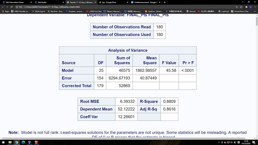
Now, we get the least square equation of our regression model from SAS:

 = 52.122 + 10.1837 1 + 1.31957 2 + 2.25778 3 + 0.523 4 + 0.58895 5
 + 0.7976 6 − 0.49193 7 − 0.13768 8 − 0.6441 9 + 0.23822 10
 + 1.94281 11 + 0.75817 12 + 0.65934 13 + 0.04247 14
 − 0.51823 15 − 0.18936 16 − 0.13833 17 + 0.78929 18
 + 0.06089 19 − 0.05777 20 − 0.09977 21 + 0.64542 22
 + 1.11766 23 + 0.55455 24 − 0.58511 25

 Figure 4 – SAS Report (1) of Model I

From the report of regression in SAS, we found that the Root MSE (Mean-square
error) is 6.39332, which is our random error ( ). It means the difference between
predicted final points and real final points is within 2 = 2 6.39332 = 12.78664.

5 Model Evaluation I

This chapter would mainly focus on determine whether our regression model is precise
or not. This chapter is consisting of two parts: residual analysis and coefficient of
determination.

5.1 Residual Analysis I

Residual analysis is a process that determine whether our regression model is precise or
not. Recall that there are some assumptions of error ( ) are needed in the regression
model in order to draw the statistical inferences, as
 ~ (0, 2 )
We need to check whether the assumptions satisfied or not.

Residual, which is our error ( ), means the difference between our target value and
the observed value ( ). Every single data point has only one residual. The equation is
as the following.
 = − 
 
Both mean and sum of residual are exactly equal to 0. Which means =0 = 0 and
 = 0.

We need to check whether the residuals be normally distributed and uncorrelated or
not by normality and homogeneity.

For normality, we are going to check the normal probability plot. Normal probability
plot is describing the residuals against our target values given their rank. If the
residuals are normally distributed, which means it has a straight line.

 Figure 5 – Normal Probability Plot of Model I

We can clearly see that, in the right plot, it shows us against . In the left plot, the
residual is normal distributed as the plot contains a straight line.

 Figure 6 – Normal Distribution Bar Graph of Model I

In figure 5, We can clearly see that the residual is following normal distribution, which
is satisfied our first part of assumption.

For homogeneity, we are going to check the residual plots. The residual plot should be
homogeneity if there is no pattern or trend. It would be separated into two parts, one is
residual against plot is describing the residual against our target values . The
second part is describing the residual against our predictors ( 1 , 2 , … , 25 ).

 Figure 7 – Residual Plot of ε against of Model I

In figure 6, we can clearly see that there are no trend or pattern between the residual
 and our target values .

Figure 8 – Residual Plot of against 1 , 2 , … , 6 of Model I

 Figure 9 – Residual Plot of against 7 , 8 , … , 12 of Model I

Figure 10 – Residual Plot of against 13 , 14 , … , 18 of Model I

Figure 11 – Residual Plot of against 19 , 20 , … , 24 of Model I

 Figure 12 – Residual Plot of against 25 of Model I

For won 1 , drew 2 , red 21 , the longest winning streak 22 , the longest
unbeaten streak 23 , the longest no-won streak 24 , and the longest losing
streak 25 , these might look different from the others plot since we got different
measurements of every single . However, there is no any systematic trend or
pattern that is non-linearity.

So, from figure 4 to figure 11, we can conclude that our regression model fulfills the
assumption of residual such that our model is trustful.

5.2 Coefficient of Determination I

The coefficient of determination 2 is also a key process of regression analysis. It is
useful to check whether the regression model is precise or not.

For R-squared 2 , it is a statistical measure that measuring the variance proportion
for target variable which can be explained by our predictors ( 1 , 2 , … , ). The
equation is as the following.
 
 2 = 1 −
 
with = =1( − )2 and = =1( − )2 .

The 2 is the square of correlation between our target variable and the
observed value . The range is from 0 to 1. If 2 = 0, it means can’t be predicted
by the predictors. If 2 = 1, it means can be predicted by the predictors without any
error. So, if 2 is close to 1, it means the regression model is precise.

Recall that, from figure 3, we found that for the model of 09/10 – 17/18 season,
the 2 = 0.8809, it means that 88.09% of observed variation can be explained by our
regression model.

For the data of 09/10 – 18/19 season, which is used to predict the 19/20 result,
the 2 = 0.8866 as the following figure 12. It means that both regression models are
trustworthy for our thesis.

 Figure 13 - SAS Report (2) of Model I

6 Result of Model I

This chapter would focus on the result of prediction from the regression model. There
are two results below. One is the prediction of 18/19 season, second one is the
prediction of 19/20 season. For 18/19 season, it is tested by 180 observations from
09/10 to 17/18. For 19/20 season, it is tested by 200 observations from 09/10 to 18/19.

There are 20 clubs each season and the ranking are rank by points, which means
getting higher points, higher rank. In order to make the prediction table to be easier to
understand, this chapter will use different color to separate the ranking in reality.

 Top Rank 1 – 4
 Rank 5 – 8
 Rank 9 – 12
 Rank 13 – 16
 Last Rank 17 – 20
 Figure 13 – Sample of Real Ranking Table

For top 4 football teams in real, I would use green color to mark them, which means
they are qualified to join UCL.

For rank 5 – 8 teams, I would use yellow to mark them, which means they have a
chance to join UEL.

For 9 – 12 teams, I would use red color to mark them. For 13 – 16 teams, I would use
blue color to mark them.

For the last 17 – 20 teams, I would use grey color to mark them, which means they
need to drop down to tier 2 English football league.

19/20 18/19
 Team Prediction Real Team Prediction Real
 Rank Points Rank Points Rank Points Rank Points
Liverpool 1 97.7 1 99 Liverpool 1 85.9 2 97
Man City 2 76.1 2 81 Man City 2 82.7 1 98
Lei City 3 74.6 5 62 Chelsea 3 74.8 3 72
Chelsea 4 66.9 4 66 Hotspur 4 70.5 4 71

Man United 5 58.6 3 66 Arsenal 5 67.8 5 70
Wolves 6 55.4 7 59 Man United 6 58.2 6 66
Hotspur 7 55.4 6 59 Everton 7 54.3 8 54
Arsenal 8 51.5 8 54 Wolves 8 53.1 7 57

Sheffield 9 51.3 10 56 Lei City 9 51.6 9 52
Everton 10 46.6 12 49 Watford 10 51.1 11 50
C. Palace 11 46.3 14 43 West Ham 11 51.0 10 52
Southampton 12 45.2 11 52 C. Palace 12 50.0 12 49

West Ham 13 44.0 16 39 Bournemouth 13 44.9 13 45
Brighton 14 43.2 15 41 Southampton 14 42.4 16 39
Burnley 15 42.3 9 54 Brighton 15 40.6 17 36
Newcastle 16 42.1 13 44 Newcastle 16 38.4 14 45
Aston Villa 17 41.4 17 35 Huddersfield 17 33.9 20 16
Bournemouth 18 37.1 18 34 Cardiff 18 33.7 18 34
Norwich 19 35.5 20 21 Fulham 19 32.2 19 26
Watford 20 33.9 19 34 Burnley 20 30.4 15 40

 Table 9 – Result of Model I

7 Model Reforming

This chapter would focus on improve and develop a new regression model by our
original model. The aim of this chapter is to try to construct a more effective and more
precise model. The techniques we use are (1) checking multi-collinearity and (2)
stepwise regression method.

7.1 Multi-collinearity

Multi-collinearity is an occurrence that there exist high inter-correlations between two
or more predictors in the regression model. Multi-collinearity would make the
predicted result to be misleading. The result of model would be unstable and given
some changes.

The method we use is Variance Inflation Factor (VIF). It is a method to check multi-
collinearity for every single predictor. The higher VIF value means higher correlation
between the predictors. The equation we use is as following.

 1
 = , = 1,2, ⋯ 
 1 − 2

where 2 is the coefficient of determination for ℎ predictor.

If > 10, it means that there exists high correlation between those and other
predictors which needs to be fixed.

Parameter Estimates

 1 21.19002 10 28.39601 19 2.01099

 2 4.09251 11 18.70659 20 1.47441

 3 12.1252 12 7.78576 21 1.21164

 4 14.06843 13 2.28117 22 4.13565

 5 6.70586 14 3.89876 23 3.92448

 6 3.04517 15 2.148 24 2.97426

 7 1.64342 16 1.6085 25 3.12884

 8 3.35813 17 1.74578

 9 1.50899 18 19.67835

 Table 10 – VIF

By table 10, after calculating the VIF value of each predictors by SAS program, we
found that the number of won ( 1 ), goal differences ( 3 ), number of shot ( 4 ),
number of pass ( 10 ), number of key pass ( 11 ), and % of possession ( 18 ), those
VIF values are greater than 10. Which means that those predictors have a high
correlation with other variables.

So, we need to determine which pair of predictors should us dealing with. We need to
check their correlation between every single predictor.

Person Correlation Coefficients, = 180
 > under 0 : ℎ = 0
 Won ⋯ Goal Difference Number of Shot ⋯ Number Number of Key ⋯ Possession ⋯
 of Pass Pass %

 Won 1 ⋯ 0.91793 0.70557 ⋯ 0.64143 0.67610 ⋯ 0.63823 ⋯

 ⋮ ⋮ ⋯ ⋮ ⋮ ⋯ ⋮ ⋮ ⋯ ⋮ ⋯

 Goal 0.91793 ⋯ 1 0.73560 ⋯ 0.68836 0.71599 ⋯ 0.68778 ⋯
Difference

 Number 0.70557 ⋯ 0.73560 1 ⋯ 0.72686 0.93659 ⋯ 0.32428 ⋯
 of Shot

 ⋮ ⋮ ⋯ ⋮ ⋮ ⋯ ⋮ ⋮ ⋯ ⋮ ⋯

 Number 0.64143 ⋯ 0.68836 0.72686 ⋯ 1 0.68405 ⋯ 0.94265 ⋯
 of Pass

 Number 0.67610 ⋯ 0.71599 0.93659 ⋯ 0.68405 1 ⋯ 0.76185 ⋯
 of Key

 Pass

 ⋮ ⋮ ⋯ ⋮ ⋮ ⋯ ⋮ ⋮ ⋯ ⋮ ⋯

Possession 0.63823 ⋯ 0.68778 0.32428 ⋯ 0.94265 0.76185 ⋯ 1 ⋯

 %

 ⋮ ⋮ ⋮ ⋮ ⋮ ⋮ ⋮ ⋮ ⋮ ⋮ ⋱

 Table 11 – Correlation Coefficient

 After calculating the coefficient by SAS, we found that number of won 1 has high
 correlation with goal difference ( 3 ). As the number of won and goal difference are
 two different indicators that very essential to a football league, so we would not deal
 with them.

 For the number of shot 4 and the number of key pass 11 , as key pass is denoted
 as assist or pass-cum-shot, means when key passing number increases, shot number
 increases, So, we would only consider number of shot ( 4 ). For number of
 pass 10 and % of possession ( 18 ), when a team has a higher possession rate, which
 means they get the ball for a longer time. In a word, they would have a higher passing
 number. So, we would only consider one of them. We have chosen number of
 pass 10 for consideration.

Parameter Estimates

 1 21.18311 10 923417 21 1.20611

 2 4.06739 12 7.50583 22 4.12053

 3 12.07777 13 2.21051 23 3.85683

 4 4.98750 14 3.80409 24 2.97043

 5 5.84718 15 2.09526 25 3.10425

 6 3.02930 16 1.56892

 7 1.64193 17 1.58008

 8 3.02930 19 1.83172

 9 1.39665 20 1.46409

 Table 12 – Updated VIF

After dealing with multi-collinearity, we have considered less two predictors which have
higher correlation to each other.

7.2 Stepwise Regression Method

Stepwise regression method is a combination of backward and forward regression
selection method. It is a useful method for choosing the predictors for fitting the
regression model. In stepwise method, the predictors are considered for addition or
subtraction. The goal for this method is to select the most powerful predictors that
affecting the result.

We are going to choose the result by having the highest coefficient of
determination ( 2 ), since the highest 2 means most of the target variables can be
explained.

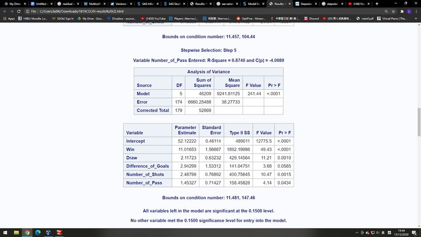
Figure 14 – Summary of Stepwise Selection

 Figure 15 – Stepwise Result

By SAS, we found that, when adding up number of won 1 , number of drew 2 ,
goal difference 3 , number of shot 4 , and number of pass 10 , the 2 is the
highest which is 0.8740.

8 Model Evaluation II

This chapter is focusing on the determining whether the new regression model is
precise or not. The method we use is residual analysis and coefficient of determination.

8.1 Residual Analysis II

For normality, we are going to check the normal probability plot.

 Figure 16 – Normal Probability Plot of Model II

We can clearly see that, in the left plot, the residual is normal distributed as the plot
contains a straight line.

 Figure 17 – Normal Distribution Bar Graph of Model II

In figure 17, we can clearly see that the residual is following normal distribution, which
is satisfied our first part of assumption.

For homogeneity, we are going to check the residual plots.

 Figure 18 - Residual Plot of against of Model II

In figure 18, we can clearly see that there are no trend or pattern between the residual
 and our target values .

 Figure 19 - Residual Plot of against 1 , 2 , 3 , 4 10 of Model I

In figure 10, we can clearly see that there are no trend or pattern between the residual
 and our predictors.

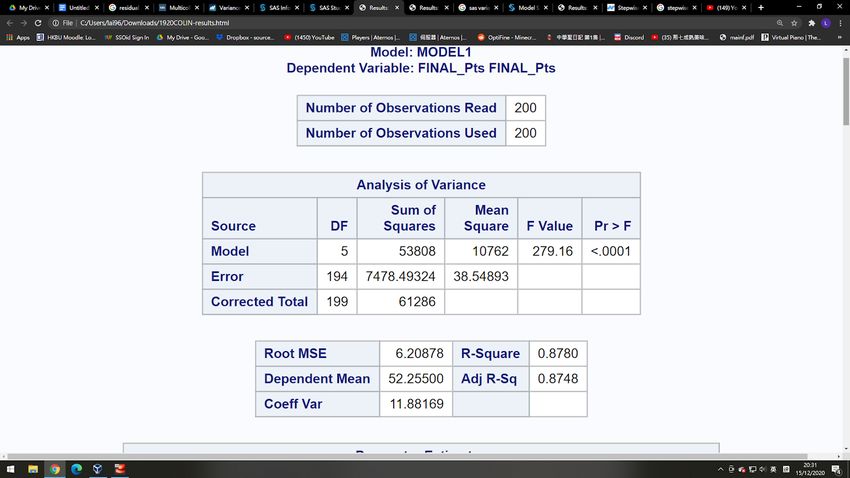
8.2 Coefficient of Determination II

Recall that, from figure 14, we found that for the model of 09/10 – 17/18 season,
the 2 = 0.8740, it means that 87.4% of observed variation can be explained by our
regression model.

For the data of 09/10 – 18/19 season, which is used to predict the 19/20 result,
the 2 = 0.8780 as the following figure 12. It means that both regression models are
trustworthy for our thesis.

 Figure 12 - SAS Report (2) of Model II

9 Model Description II

By checking multi-collinearity and stepwise selection, we have constructed a new
regression model with 5 predictors.

Dependent Variable ( )

 Dependent Variable Data Description
 Final Points each team for whole season
 Table 13 – Dependent Variable ( )

Independent Variable ( )

 Independent Variable Data Description
 1 Number of Won
 2 Number of Drew
 3 Goal Difference
 4 Number of Shot
 5 Number of Pass
 Table 14 – Independent Variable ( )

Regression Coefficient 
 Regression Coefficients ( )
 0 52.1222
 1 11.01653
 2 2.11723
 3 2.94299
 4 2.48799
 5 1.45327
 Table 15 – Regression Coefficient of Model II

Least Square Equation
 = 52.1222 + 11.01653 1 + 2.11723 2 + 2.94299 3 + 2.48799 4 + 1.45327 5

10 Result of Model II

 This chapter would focus on the result of prediction from the new regression model.
 There are two results below. One is the prediction of 18/19 season, second one is the
 prediction of 19/20 season. For 18/19 season, it is tested by 180 observations from
 09/10 to 17/18. For 19/20 season, it is tested by 200 observations from 09/10 to 18/19.

 19/20 18/19
 Team Prediction Real Team Prediction Real
 Rank Points Rank Points Rank Points Rank Points
Liverpool 1 93.8 1 99 Liverpool 1 84.0 2 97
Man City 2 80.9 2 81 Man City 2 81.0 1 98
Lei City 3 72.5 5 62 Chelsea 3 74.1 3 72
Chelsea 4 65.7 4 66 Hotspur 4 70.8 4 71

Man United 5 58.4 3 66 Arsenal 5 66.7 5 70
Wolves 6 56.6 7 59 Man United 6 59.7 6 66
Hotspur 7 56.5 6 59 Everton 7 53.9 8 54
Sheffield 8 52.8 10 52 Lei City 8 52.5 9 52

Arsenal 9 49.3 8 56 Wolves 9 52.4 8 57
C. Palace 10 47.4 14 43 West Ham 10 50.4 10 52
Everton 11 46.3 12 49 Watford 11 50.3 11 50
Brighton 12 45.3 15 41 Bournemouth 12 48.3 13 45

Newcastle 13 44.0 13 44 C. Palace 13 44.1 12 49
Burnley 14 43.8 9 54 Southampton 14 42.1 16 39
Southampton 15 42.7 11 52 Brighton 15 41.8 17 36
Bournemouth 16 42.0 18 34 Newcastle 16 38.9 14 45

Aston Villa 17 41.7 17 35 Cardiff 17 34.6 18 34
West Ham 18 40.5 16 39 Fulham 18 34.5 19 26
Norwich 19 33.3 20 21 Huddersfield 19 32.8 20 16
Watford 20 31.6 19 34 Burnley 20 29.2 15 40

 Table 16 – Result of Model II

11 Comparison of Model I and Model II

In this chapter, it would focus on the comparison of model I and model II, which are
before development and after development. We can determine which of the model is
more accuracy.

We would consider in 6 indicators: (1) number of correct predicted team in top 4 and
last 4, (2) number of correct predicted team in 5 – 8, (3) number of correct team in 9 –
16, (4) absolute point difference, (5) ranking difference, (6) number of correct position.

For (1), it is important that, for top 4 football team, it explained that they are qualified
to join UEFA Champions League. For last 4 football team, it explained that they need
to drop off to EFL Championship. The higher number means the higher accuracy.

For (2), it is important that, for rank 5 – 8 team, it explained that they have a chance to
join UEFA Europa League. The higher number means the higher accuracy.

For (3), for team 9 – 16, it explained the remaining team rank. The higher number
means the higher accuracy.

For (4), as our target variable is final point, so it is necessary to determine the accurate
of model. The lower number means the higher accuracy.

For (5), we determine the rank difference between our predicted ranking and real
ranking. The lower number means the higher accuracy.

For (6), we determine the number of correct position of our predicting position. The
higher number means the higher accuracy.

For Model I,
 Model I
 (1) (2) (3) (4) (5) (6)
 18/19 7 4 7 99 20 9

 19/20 7 3 6 99 28 5

 Total 14 7 13 198 48 14

 Table 17 – Efficacy of Model I

For Model II,
 Model II
 (1) (2) (3) (4) (5) (6)
 18/19 7 3 4 109 21 6

 19/20 6 2 2 98 32 4

 Total 13 5 6 207 53 10

 Table 18 – Efficacy of Model II

After comparison, we found that model I is more accuracy than model II while model I
have a greater performance of prediction power.

However, we can see that for (1), model II can predict correctly for 13 football teams
while model I has 14. But, model II only consider 5 independent variables while model
I considers 25. It shows us model II is effective also.

All in all, in this thesis, we can conclude that model I is more accurate and model II is
more effective.

12 Prediction of 20/21 Final Ranking Table

Here is my prediction of 20/21 final ranking table by applying model I.

 Team Prediction
 Rank Points
 Man City 1 68.6
 Liverpool 2 67.3
 Man United 3 66.5
 Lei City 4 63.2
 Hotspur 5 62.9

 Everton 6 61.5
 Chelsea 7 61.2
 Aston Villa 8 60.2

 West Ham 9 57.0
 Southampton 10 56.2
 Leeds 11 52.8
 Wolves 12 52.5

 Newcastle 13 48.1
 Arsenal 14 46.5
 Crystal Palace 15 46.3
 Fulham 16 40.8

 Burnley 17 39.8
 Brighton 18 34.8
 West Brom 19 32.1
 Sheffield United 20 29.3

 Table 18 – 20/21 Prediction Table

13 Discussion of Limitation

This chapter would mainly focus on the limitation of our regression model for
predicting the final table.

Unexpected Incidents in Second Half Season

First, as we are going to use only the data of the first half season, which is the first 19
matches for each team, the unexpected incidents happening in the second half season
cannot be considered.

For instance, every single team can change the manager or coach in order to get a better
result. The tactics and strategy can be changed due to the different coaches. Also, each
club can sign new players or some players leave in the winter transfer window, which is
held from the middle of season. It may lead to a different score between the first half
and second half.

To take Manchester United F.C. (Man United) in 19/20 as an example, in the first half
of season, they were in rank 8 in real. For my prediction, Man United would get rank 5.
However, Man United signed a new attacking midfielder, Bruno Fernandes, in winter
transfer window. He made a huge influence on the club. He had 10 scores and 6
assists, which had a very virtuous contribution for club. He had got two Player of the
Month awards and one Goal of the Month award in 19/20 season. His contribution
helped Man United to gain a high position in final, which was rank 3.

Apart from the changing of teams, there may be some incidents that happening in the
second half, may affect the whole football league. To take the 19/20 season as an
example, on March 20, Premier League needed to be suspended for 3 months because
of COVID-19. It leads to a huge different performance of each team between before
suspension and after resumption that we cannot count in. The health of players has a
huge influence on their performance. Also, during the suspension, every single player
only could train himself, but not with the team. It might lead to a bad result for them
and for our prediction.

To take Leicester City F.C. (Lei City) in 19/20 as an example, before suspension, Lei
City had played 29 games and was in rank 3, which was close to our prediction. The
percentage of won was 55%. However, after resumption, Lei City had played 9 games
which only had 2 wins. The winning percentage was 22%. It made a huge bad influence
on the performance after resumption.

It was an unexpected and unconsidered incident that affected our accuracy, that we may
overestimate or underestimate the performance of each team.

Unconsidered Tactics of Every Team

For our regression model, number of shots ( 4 ), number of shot on targets ( 5 ),
number of pass ( 10 ), number of key pass ( 11 ), and % of Possession ( 18 ) are
essential predictors. It can easily explain as the chance for scoring. While a team wants
to score, they need to organize their attacking plan, and try to put the ball into the net.
If a team has higher number of shots on targets, the team has a higher probability to
win.

However, there are some special cases that a team having lower % of possession, and
lower shot numbers, can win the game and get 3 points. It is due to the tactics and style
of different coaches. For example, José Mourinho, a manager and head coach of PL
club Hotspur. However, his tactic is kindly different from other coaches. His tactic can
be explained as counter-attack, which abandons possession %, shot number, etc. His
tactic is focusing on fewer chances and trying to get the points.

It means that different tactics may lead to a different performance of data. It may affect
the accuracy of our model.

Unconsidered Factors

Every club would have a different length of time break between two games, due to the
international league. The length of break affects their performance in PL. However, as
our model is focusing on the final table of PL, we have not considered the break length
of each team. It may affect the accuracy of our model.

Insufficient of Prediction of Midstream Clubs

Since the performances of clubs in midstream are quite similar, i.e. in rank 9 – 16, for
example, the number of shots, the times of won, the goal differences, etc. The
difference between their points were small, which means their ranking could be
changed easily after few games. It is hard for our model to predict precisely.

 Team 19/20 First Half
 Rank Points
 ⋮ ⋮ ⋮

 C. Palace 9 26
 Newcastle 10 25
 Arsenal 11 24
 Burnley 12 24
 Everton 13 22
 Southampton 14 21
 ⋮ ⋮ ⋮

 Table 19 – 19/20 Point Table of First Half of Season

For example, in table 19, we can see that the points of midstream clubs are quite
similar. If Burnley (rank 12) got one won later, which means they could get 3 points
more, their rank would be increased into rank 8 or even higher.

It is hard for our model to predict precisely the ranking of midstream clubs as their
performances are similar.

14 Conclusion

In this thesis, we have set up a linear regression model in order to predict the final table
of Premier League.

First, we have collected the useful data of each team from the 09/10 season to 19/20
season. We have set up a regression model I by those data and evaluate the model.

Then, in order to improve the accuracy and efficiency of our model, we have checked
the multi-collinearity and have done the stepwise regression method. We have set up a
new model II that only contains 5 predictors.

After that, we have compared the accuracy between model I and model II. We found
that model I is more precise while model II is more effective.

Finally, we used model I to predict the result of the 20/21 final ranking table.

15 Reference

Joel, O., “Differentiating the Top English Premier League Football Clubs from
 the Rest of the Pack: Identifying the Keys to Success” (2009), Journal of Quantitative
 Analysis in Sports: Vol. 5, No. 3, Article 10.

Christos, T. and Victor, C., “Sports Analytics for Football League Table and Player
 Performance Prediction” (2020), School of Science and Technology, International
 Hellenic University.

Carlos, P. B. and Stephanie, L., “Performance evaluation of the English Premier
 Football League with data envelopment analysis” (2006), Applied Economics,
 Vol. 38.

Wray, V., “Creating the English Premier Football League: A Brief Economic
 History with Some Possible Lessons for Asian Soccer” (2017), International Journal
 of the History of Sport, Vol. 34, pp. 17-18.

Mike, W., “Determining the Best Strategy for Changing the Configuration of a
 Football Team” (2003), Journal of the Operational Research Society, Vol. 54.