Recognizing Landmarks in Large-Scale Social Image Collections
←
→
Page content transcription
If your browser does not render page correctly, please read the page content below
Recognizing Landmarks in Large-Scale Social
Image Collections

David J. Crandall, Yunpeng Li, Stefan Lee, and Daniel P. Huttenlocher

Abstract The dramatic growth of social media websites over the last few years has
created huge collections of online images and raised new challenges in organizing
them effectively. One particularly intuitive way of browsing and searching images
is by the geo-spatial location of where on Earth they were taken, but most online
images do not have GPS metadata associated with them. We consider the problem
of recognizing popular landmarks in large-scale datasets of unconstrained consumer
images by formulating a classification problem involving nearly 2 million images
and 500 categories. The dataset and categories are formed automatically from geo-
tagged photos from Flickr by looking for peaks in the spatial geotag distribution
corresponding to frequently photographed landmarks. We learn models for these
landmarks with a multiclass support vector machine, using classic vector-quantized
interest point descriptors as features. We also incorporate the non-visual metadata
available on modern photo-sharing sites, showing that textual tags and temporal
constraints lead to significant improvements in classification rate. Finally, we ap-
ply recent breakthroughs in deep learning with Convolutional Neural Networks,
finding that these models can dramatically outperform the traditional recognition
approaches to this problem, and even beat human observers in some cases.1

David J. Crandall
Indiana University, Bloomington, Indiana USA, e-mail: djcran@indiana.edu
Yunpeng Li
École Polytechnique       Fédérale   de   Lausanne,   1015   Lausanne,    Switzerland,   e-mail:
yunpeng.li@epfl.ch
Stefan Lee
Indiana University, Bloomington, Indiana USA, e-mail: steflee@indiana.edu
Daniel P. Huttenlocher
Cornell University, Ithaca, New York USA, e-mail: dph@cs.indiana.edu
1   This is an expanded and updated version of an earlier conference paper [23].

                                                                                                 1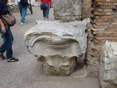
2                       David J. Crandall, Yunpeng Li, Stefan Lee, and Daniel P. Huttenlocher

1 Introduction

Online photo collections have grown dramatically over the last few years, with Face-
book alone now hosting over 250 billion images [2]. Unfortunately, techniques for
automatic photo organization and search have not kept pace, with most modern
photo-sharing sites using simple techniques like keyword search based on text tags
provided by users. In order to allow users to browse and search huge image collec-
tions more efficiently we need algorithms that can automatically recognize image
content and organize large-scale photo collections accordingly.
   A natural way of organizing photo collections is based on geospatial location —
where on Earth an image was taken. This allows people to search for photos taken
near a particular spot of interest, or to group images based on similar locations or
travel itineraries. To enable this type of organization, geospatial coordinates or ‘geo-
tags’ can be encoded in the metadata of a photo, and Global Positioning System
(GPS) receivers embedded in modern smartphones and high-end cameras can record
these positions automatically when a photo is captured. However, the vast majority
of online photos are not geo-tagged, and even when available, geo-tags are often
incorrect due to GPS error or other noise [15].
   Recognizing where a photo was taken based on its visual content is thus an im-
portant problem. Besides the potential impact on geo-localization, this is an in-
teresting recognition problem in and of itself. Unlike many tasks like scene type
recognition or tag suggestion, which are inherently subjective, place recognition is
a uniquely well-posed problem; except for pathological cases like synthetic images
or photos taken from space, every photo is taken at exactly one point on Earth, and
so there is exactly one correct answer. Moreover, it is relatively easy to assemble
large-scale training and test data for this problem by using geo-tagged images from
social media sites like Flickr. This is in contrast to most other recognition prob-
lems in which producing ground truth data involves extensive manual labor, which
historically has limited the size of datasets and introduced substantial bias [38].
   In this chapter we consider the problem of classifying consumer photos accord-
ing to where on Earth they were taken, using millions of geo-tagged online im-
ages to produce labeled training data with no human intervention. We produce this
dataset by starting with a collection of over 30 million public geo-tagged images
from Flickr. We use this dataset both to define a set of category labels, as well as to
assign a ground truth category to each training and test image. The key observation
underlying our approach is that when many different people take photos at the same
place, they are likely photographing some common area of interest. We use a mean
shift clustering procedure [4] to find hotspots or peaks in the spatial distribution of
geotagged photos, and then use large peaks to define the category labels. We then
assign any photos geo-tagged within a peak to the same category label.
   We call each localized hotspot of photographic activity a landmark. Most of our
landmarks do not consist of a single prominent object; for example, many are muse-
ums, with photos of hundreds of different exhibits as well as photos containing little
or no visual evidence of the landmark itself (e.g. close-ups of people’s faces). We
could use visual or textual features of images to try to divide these complex land-
Recognizing Landmarks in Large-Scale Social Image Collections                        3

marks into individual objects, as others have done [42], but we purposely choose
not to do this; by defining the labels using only geo-tags, we ensure that the fea-
tures used for testing classification algorithms (namely visual content, text tags, and
timestamps) do not also bias the category labels. However, because we do not try
to remove outliers or difficult images, the photographs taken at these landmarks are
quite diverse (see Figure 1 for some examples), meaning the labeled test datasets are
noisy and challenging. Our landmark classification task is thus more similar to ob-
ject category recognition than to specific object recognition. In Section 3 we discuss
the details of our dataset collection approach.
    Once we have assembled a large dataset of millions of images and hundreds
of categories, we present and evaluate techniques for classifying the landmark at
which each photo was taken. We first apply multiclass Support Vector Machines
(SVMs) [5] with features based on classic bags of vector-quantized invariant fea-
ture point descriptors [8, 25]. Social photo collections also contain sources of non-
visual evidence that can be helpful for classification; for instance, social ties have
been found to improve face recognition [36] and image tagging [27]. We explore
incorporating the free-form text tags that Flickr users add to some photos. We also
incorporate temporal evidence, using the fact that most people take series of pho-
tos over time (for instance, as they move about the tourist sites of a city). We thus
analyze the photo stream of a given photographer, using Structured Support Vector
Machines [40] to predict a sequence of category labels jointly rather than classifying
a single photo at a time. Finally, inspired by the very recent success of deep learning
techniques on a variety of recognition problems [20, 29, 37, 39], we apply Convolu-
tional Neural Networks to our problem of landmark classification as an alternative
to the more traditional bag-of-words models with hand-designed image features.
Feature extraction, learning, and classification methods are discussed in Section 4.
    In Section 5 we present a set of large-scale classification experiments involving
between 10 and 500 categories and tens to hundreds of thousands of photos. We
begin with the bag-of-words models of SIFT feature points, finding that the combi-
nation of image and text features performs better than either alone, and that visual
features boost performance even for images that already have text tags. We also de-
scribe a small study of human accuracy on our dataset, to give a sense of the noise
and difficulty of our task. We then show that using temporal context from photos
taken by the same photographer nearby in time yields a significant improvement
compared to using visual features alone — around 10 percentage points in most
cases. Finally, we show that the neural nets give a further dramatic increase in per-
formance, in some cases even beating humans, giving further evidence of the power
of deep learning over traditional features on problems with large-scale datasets.

2 Related Work

Visual geolocation has received increasing attention in the last few years [14,16,19,
22–24,30,31,35,42] driven in part by the availability of cheap training and test data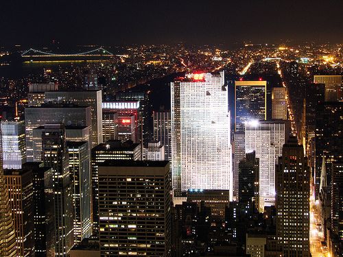
4                      David J. Crandall, Yunpeng Li, Stefan Lee, and Daniel P. Huttenlocher

in the form of geo-tagged Flickr photos. We briefly highlight some of the work most
related to this chapter here, but please see Luo et al. [26] for a more comprehensive
survey. The IM2GPS paper of Hays and Efros [16] estimates a latitude-longitude
coordinate estimate for an image by matching against a large dataset of geo-tagged
photos from Flickr, identifying nearest neighbors and producing a geospatial prob-
ability distribution based on the matches. Our goal is different, as we do not try to
predict location directly but rather just use location to derive category labels. (For
instance, in our problem formulation a misclassification with a geographically prox-
imate category is just as bad as with one that is far away.) Moreover, the IM2GPS
test set contains only 237 images that were partially selected by hand, making it
difficult to generalize the results beyond that set. In contrast we use automatically
generated test sets that contain tens or hundreds of thousands of photos, provid-
ing highly reliable estimates of performance accuracy. Follow-up work by Kaloger-
akis et al. generalized IM2GPS to geo-localize a stream of multiple images at the
same time by imposing constraints on human travel patterns [19].
    Other papers have considered landmark classification tasks similar to the one we
study here, although typically at a smaller scale. For example, Li et al. [22] study
how to build a model of a landmark by extracting a small set of iconic views from
a large set of photographs. The paper tests on three hand-chosen categories. Zheng
et al. [42] have an approach similar to ours in that it finds highly photographed
landmarks automatically from a large collection of geotagged photos. However, the
test set they use is hand-selected and small — 728 total images for a 124-category
problem, or fewer than 6 test images per category — and their approach is based
on nearest-neighbor search, which may not scale to the millions of test images we
consider here. Philbin et al. [30] study building recognition in the context of how
to scale bag-of-features models using random vocabulary trees and fast geometric
verification, testing on a dataset of 5,000 labeled images. Crandall et al. [6] study
geographic embedding and organization of photos by clustering into landmarks and
also study recognition, but at a much more limited scale (classifying among land-
marks of a known city).
    While we approach geo-localization as a recognition problem, an alternative is
to study it in the context of 3D reconstruction [35]. If a 3D model of a place is
available, then new images can be geo-localized very accurately, sometimes much
more accurately than GPS [7]. But 3D reconstruction is computationally expensive,
and is possible only in areas having dense coverage (typically thousands of images).
    We apply several widely used recognition techniques to our landmark recogni-
tion problem, based on bag-of-words models of vector-quantized, invariant feature
points [8, 25]. A very large body of literature has studied these models, includ-
ing how to optimize them for accuracy and speed in different contexts and tasks:
see Grauman and Leibe [12] for a comprehensive overview. We also apply Con-
volutional Neural Networks, which, in contrast, are arguably less well understood.
Following the surprising success of deep Convolutional Neural Networks on the
2012 ImageNet recognition challenge [20], CNNs have been applied to a variety
of computer vision tasks and have shown striking improvements over the state of
the art [11, 21, 29, 32, 34, 37, 39, 41]. The main advantage of deep learning methods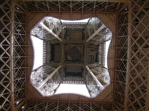
Recognizing Landmarks in Large-Scale Social Image Collections                         5

over more traditional techniques is that the image features can be learned along with
the object models in a unified optimization problem, instead of using generic hand-
designed features (like SIFT [25]), which are likely not optimal for most tasks. Of
course, learning these features requires more data and more computational power;
the resurgence of neural networks in computer vision is thanks in no small part to
powerful GPUs and large annotated datasets (like the ones we have here).

3 Building an Internet-Scale Landmark Dataset

Social photo-sharing websites with their huge collections of publicly available, user-
generated images and metadata have been a breakthrough in computer vision, giving
researchers an economical way of collecting large-scale, realistic consumer imagery.
However, when constructing datasets from Internet photo sources, it is critical to
avoid potential biases either in selecting the images to include in the dataset, the
categories to include in the classification task, or in assigning ground-truth labels to
images. Biases of different types affect even the most popular vision datasets [38].
For instance, methods based on searching for photos tagged with hand-selected key-
words (e.g., [16, 30]) are prone to bias, because one might inadvertently choose
keywords corresponding to objects that are amenable to a particular image classifi-
cation algorithm. Many researchers have also used unspecified or subjective crite-
ria to choose which images to include in the dataset, again introducing the poten-
tial for bias towards a particular algorithm. Other object recognition datasets like
PASCAL [10] and Caltech [13] have object classes that were selected by computer
vision researchers, making it unclear whether these are the most important cate-
gories that should be studied. Also problematic is using the same kinds of features
to produce ground-truth labels as are used by the classification algorithm [3, 33, 42].
Recent datasets like ImageNet [9] avoid many sources of bias by defining ground
truth labels based on more principled approaches like semantic categories of Word-
Net [28], and by avoiding subconscious biases of computer vision researchers by
crowd-sourcing labels with Mechanical Turk, but these approaches still require a
huge amount of human labor.
    We thus advocate automatic techniques for creating datasets based on properties
of human activity, such as where pictures are taken, without manual intervention. To
be most useful for training and testing of classifiers, the ground truth labels should
be selected and produced in a way that is automatic and objective, based on sources
other than the features used by the classifiers. Our approach is based on the observa-
tion that when many people take photos at the same location it is highly likely that
these are photos of the same thing. We therefore define category labels by finding
geospatial clusters of high photographic activity and assign all photos within that
cluster the same label.
    In particular, our dataset was formed by using Flickr’s public API to retrieve
metadata for over 60 million publicly accessible geotagged photos. We eliminated
photos for which the precision of the geotags was worse than about a city block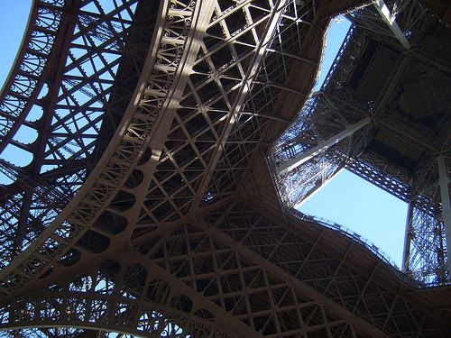
6 David J. Crandall, Yunpeng Li, Stefan Lee, and Daniel P. Huttenlocher
1. eiffeltower random tags: eiffel, city, travel, night, street
2. trafalgarsquare random tags: london, summer, july, trafalgar, londra
3. bigben random tags: westminster, london, ben, night, unitedkingdom
4. londoneye random tags: stone, cross, london, day2, building
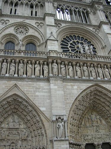
5. notredame random tags: 2000, portrait, iglesia, france, notredamecathedral
6. tatemodern random tags: england, greatbritian, thames, streetart, vacation
7. empirestatebuilding random tags: manhattan, newyork, travel, scanned, evening
8. venice random tags: tourists, slide, venecia, vacation, carnival
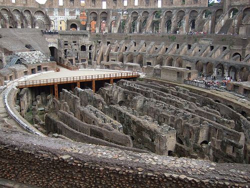
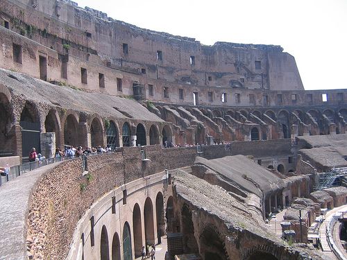
9. colosseum random tags: roma, england, stadium, building, italy
10. louvre random tags: places, muséedulouvre, eau, paris, canon
Fig. 1 The categories in our 10-way classification dataset, consisting of the 10 most photographed
landmarks on Flickr. To illustrate the diversity and noise in our automatically generated dataset, we
show five random images and five random text tags from each category. (We have obscured faces
to protect privacy. The landmark tagged “venice” is Piazza San Marco.)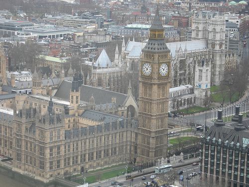
Recognizing Landmarks in Large-Scale Social Image Collections                                                                        7
     Users    Geo-coordinate      Descriptive tags                       Users     Geo-coordinate     Descriptive tags
 1    4854      48.8584, 2.2943   eiffeltower, paris                51    1391     41.8991, 12.4730   piazzanavona, rome
 2    4146     51.5080, -0.1281   trafalgarsquare, london           52    1379     41.9061, 12.4826   spanishsteps, rome
 3    3442     51.5008, -0.1243   bigben, london                    53    1377   37.8026, -122.4060   coittower, sanfrancisco
 4    3424     51.5034, -0.1194   londoneye, london                 54    1369    40.6894, -74.0445   libertyisland, newyorkcity
 5    3397      48.8531, 2.3493   cathedral, paris                  55    1362     41.8953, 12.4828   vittoriano, rome
 6    3369     51.5080, -0.0991   tatemodern, london                56    1359     51.5050, -0.0790   cityhall, london
 7    3179    40.7485, -73.9854   empirestatebuilding, newyorkcity  57    1349      50.8467, 4.3524   grandplace, brussel
 8    3167     45.4340, 12.3390   venice, venezia                   58    1327      48.8621, 2.2885   trocadero, paris
 9    3134     41.8904, 12.4920   colosseum, rome                   59    1320   36.1016, -115.1740   newyorknewyork, lasvegas
10    3081      48.8611, 2.3360   pyramid, paris                    60    1318      48.8656, 2.3212   placedelaconcorde, paris
11    2826    40.7578, -73.9857   timessquare, newyorkcity          61    1320     41.9024, 12.4663   castelsantangelo, rome
12    2778    40.7590, -73.9790   rockefeller, newyorkcity          62    1305     52.5094, 13.3762   potsdamerplatz, berlin
13    2710    41.8828, -87.6233   cloudgate, chicago                63    1297    41.8892, -87.6245   architecture, chicago
14    2506     41.9024, 12.4574   vaticano, rome                    64    1296    40.7613, -73.9772   museumofmodernart, newyorkcity
15    2470      48.8863, 2.3430   sacrecoeur, paris                 65    1292     50.0865, 14.4115   charlesbridge, praha
16    2439     51.5101, -0.1346   piccadillycircus, london          66    1270    40.7416, -73.9894   flatironbuilding, newyorkcity
17    2321     51.5017, -0.1411   buckingham, london                67    1260     48.1372, 11.5755   marienplatz, mnchen
18    2298    40.7562, -73.9871   timessquare, newyorkcity          68    1242    40.7792, -73.9630   metropolitanmuseumofart, newyorkcity
19    2296      48.8738, 2.2950   arcdetriomphe, paris              69    1239      48.8605, 2.3379   louvre, paris
20    2127    40.7526, -73.9774   grandcentralstation, newyorkcity  70    1229    40.7354, -73.9909   unionsquare, newyorkcity
21    2092     41.8989, 12.4768   pantheon, rome                    71    1217    40.7541, -73.9838   bryantpark, newyorkcity
22    2081      41.4036, 2.1742   sagradafamilia, barcelona         72    1206   37.8266, -122.4230   prison, sanfrancisco
23    2020     51.5056, -0.0754   towerbridge, london               73    1196    40.7072, -74.0110   nyse, newyorkcity
24    1990    38.8894, -77.0499   lincolnmemorial, washingtondc     74    1193      45.4643, 9.1912   cathedral, milano
25    1983     51.5193, -0.1270   britishmuseum, london             75    1159     40.4155, -3.7074   plazamayor, madrid
26    1960     52.5164, 13.3779   brandenburggate, berlin           76    1147     51.5059, -0.1178   southbank, london
27    1865     51.5078, -0.0762   toweroflondon, london             77    1141   37.8022, -122.4190   lombardstreet, sanfrancisco
28    1864     45.4381, 12.3357   rialto, venezia                   78    1127   37.7951, -122.3950   ferrybuilding, sanfrancisco
29    1857    40.7641, -73.9732   applestore, newyorkcity           79    1126   -33.8570, 151.2150   sydneyoperahouse, sydney
30    1828   47.6206, -122.3490   needle, seattle                   80    1104     51.4996, -0.1283   westminsterabbey, london
31    1828   47.6089, -122.3410   market, seattle                   81    1100     51.5121, -0.1229   coventgarden, london
32    1798     51.5013, -0.1198   bigben, london                    82    1093   37.7846, -122.4080   sanfrancisco, sanfrancisco
33    1789    38.8895, -77.0406   wwii, washingtondc                83    1090    41.8988, -87.6235   hancock, chicago
34    1771     50.0873, 14.4208   praga, praha                      84    1083     52.5141, 13.3783   holocaustmemorial, berlin
35    1767     51.5007, -0.1263   bigben, london                    85    1081     50.0862, 14.4135   charlesbridge, praha
36    1760      48.8605, 2.3521   centrepompidou, paris             86    1077     50.0906, 14.4003   cathedral, praha
37    1743     41.9010, 12.4833   fontanaditrevi, rome              87    1054      41.3840, 2.1762   cathedral, barcelona
38    1707   37.7879, -122.4080   unionsquare, sanfrancisco         88    1042    28.4189, -81.5812   castle, waltdisneyworld
39    1688     43.7731, 11.2558   duomo, firenze                    89    1034    38.8898, -77.0095   capitol, washingtondc
40    1688     43.7682, 11.2532   pontevecchio, firenze             90    1024      41.3820, 2.1719   boqueria, barcelona
41    1639   36.1124, -115.1730   paris, lasvegas                   91    1023      48.8638, 2.3135   pontalexandreiii, paris
42    1629     43.7694, 11.2557   firenze, firenze                  92    1022     41.8928, 12.4844   forum, rome
43    1611    38.8895, -77.0353   washingtonmonument, washingtondc 93     1021    40.7060, -73.9968   brooklynbridge, newyorkcity
44    1567     41.9023, 12.4536   basilica, rome                    94    1011   36.6182, -121.9020   montereybayaquarium, monterey
45    1505     51.5137, -0.0984   stpaulscathedral, london          95    1009     37.9716, 23.7264   parthenon, acropolis
46    1462    40.7683, -73.9820   columbuscircle, newyorkcity       96    1008      41.3953, 2.1617   casamil, barcelona
47    1450      41.4139, 2.1526   parcguell, barcelona              97     986    43.6423, -79.3871   cntower, toronto
48    1433     52.5186, 13.3758   reichstag, berlin                 98     983     52.5099, 13.3733   sonycenter, berlin
49    1419   37.8107, -122.4110   pier39, sanfrancisco              99     972   34.1018, -118.3400   hollywood, losangeles
50    1400     51.5101, -0.0986   millenniumbridge, london         100     969      48.8601, 2.3263   museedorsay, paris

Table 1 The world’s 100 most-photographed, landmark-sized hotspots as of 2009, according to
our analysis of Flickr geo-tags, ranked by number of unique photographers. We use these hotspots
to automatically define our landmark categories. For each landmark we show the number of pho-
tographers, the latitude-longitude coordinate of the hotspot centroid, and two automatically se-
lected tags corresponding to the most distinctive tag (i.e. most-frequent relative to the worldwide
background distribution) within the landmark region and within the surrounding city-scale region.

(precision score under 13 in the Flickr metadata). For each of the remaining 30
million photos, we considered its latitude-longitude coordinates as a point in the
plane, and then performed a mean shift clustering procedure [4] on the resulting
set of points to identify local peaks in the photo density distribution [6]. The radius
of the disc used in mean shift allowed us to select the scale of the ‘landmarks.’
We used a radius of 0.001 degrees, which corresponds to roughly 100 meters at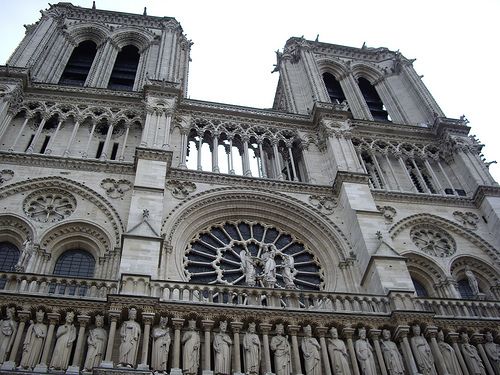
8                           David J. Crandall, Yunpeng Li, Stefan Lee, and Daniel P. Huttenlocher

middle latitudes.2 Since our goal is to identify locations where many different people
took pictures, we count at most five photos from any given Flickr user towards any
given peak, to prevent high-activity users from biasing the choice of categories.
We currently use the top 500 such peaks as categories. After finding peaks, we
rank them in decreasing order of the number of distinct photographers who have
photographed the landmark. Table 1 shows the top 100 of these peaks, including
the number of unique photographers, the geographic centroid of the cluster, and
representative tags for each cluster. The tags were chosen automatically using the
same technique as in [6], which looks for tags that occur very frequently on photos
inside a geographic region but rarely outside of it.
   We downloaded all 1.9 million photos known to our crawler that were geotagged
within one of these 500 landmarks. For the experiments on classifying temporal
photo streams, we also downloaded all images taken within 48 hours of any photo
taken in a landmark, bringing the total dataset to about 6.5 million photos. The im-
ages were downloaded at Flickr’s medium resolution level, about 0.25 megapixels.
Figure 1 shows random images from each of the top 10 landmarks, showing the
diversity of the dataset.

4 Landmark Recognition

We now consider the task of image classification in the large-scale image dataset
produced using the procedure described above. Since our landmark categories were
selected to be non-overlapping, these categories are mutually exclusive and thus
each image has exactly one correct label. We first discuss how to classifying single
images with bag-of-words models in Section 4.1, before turning to the temporal
models in Section 4.2 and the deep learning-based methods in Section 4.3.

4.1 Single Image Classification Using Bag of Words Models

To perform image classification we adopt the bag-of-features model proposed by
Csurka et al. [8], where each photo is represented by a feature vector recording oc-
currences of vector-quantized SIFT interest point descriptors [25]. As in that paper,
we built a visual vocabulary by clustering SIFT descriptors from photos in the train-
ing set using the k-means algorithm. To prevent some images or categories from
biasing the vocabulary, for the clustering process we sampled a fixed number of in-
terest points from each image, for a total of about 500,000 descriptors. We used an
efficient implementation of k-means using the approximate nearest neighbor (ANN)
technique of [1] (to assign points to cluster centers during the expectation (E-step)
2 Since longitude lines grow closer towards the poles, the spatial extent of our landmarks are larger
at the equator than near the poles. We have not observed this to be a major problem because most
population centers are near the middle latitudes, but future work could use better distance functions.
Recognizing Landmarks in Large-Scale Social Image Collections                       9

of k-means). The advantage of this technique over many others is that it guarantees
an upper bound on the approximation error; we set the bound such that the cluster
center found by ANN is within 110% of the distance from the point to the optimal
cluster center.
    Once a visual vocabulary of size k had been generated, a k-dimensional feature
vector was constructed for each image by using SIFT to find local interest points
and assigning each interest point to the visual word with the closest descriptor. We
then formed a frequency vector which counted the number of occurrences of each
visual word in the image. For textual features we used a similar vector space model
in which any tag used by at least three different users was a dimension in the feature
space, so that the feature vector for a photo was a binary vector indicating presence
or absence of each text tag. Both types of feature vectors were L2-normalized. We
also studied combinations of image and textual features, in which case the image
and text feature vectors were simply concatenated after normalization.
    We learned a linear model that scores a given photo for each category and assigns
it to the class with the highest score. More formally, let m be the number of classes
and x be the feature vector of a photo. Then the predicted label is

                            ŷ = arg maxy∈{1,···,m} s(x, y; w),                   (1)

where w = (wT1 , · · · , wTm )T is the model and s(x, y; w) = wy , x is the score for
class y under the model. Note that in our settings, the photo is always assumed to
belong to one of the m categories. Since this is by nature a multi-way (as opposed
to binary) classification problem, we use multiclass SVMs [5] to learn the model
w, using the SVMmulticlass software package [18]. For a set of training examples
{(x1 , y1 ), · · · , (xN , yN )}, our multiclass SVM optimizes an objective function,
                                   N
                           1
                      min kwk2 +C ∑ ξi                                            (2)
                      w,ξξ 2      i=1
                      s.t. ∀i, y 6= yi : wyi , xi − wy , xi ≥ 1 − ξi ,

where C is the trade-off between training performance and margin in SVM formu-
lations (which we simply set to x̄−2 where x̄ is the average L2-norm of the training
feature vectors). Hence for each training example, the learned model is encouraged
to give higher scores to the correct class label than to the incorrect ones. By rear-
ranging terms it can be shown that the objective function is an upper bound on the
training error.
    In contrast, many previous approaches to object recognition using bag-of-parts
models (such as Csurka et al. [8]) trained a set of binary SVMs (one for each cate-
gory) and classified an image by comparing scores from the individual SVMs. Such
approaches are problematic for n-way, forced-choice problems, however, because
the scores produced by a collection of independently trained binary SVMs may not
be comparable, and thus lack any performance guarantee. It is possible to alleviate
this problem by using a different C value for each binary SVM [8], but this in-
troduces additional parameters that need to be tuned, either manually or via cross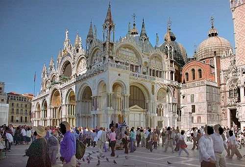
10                       David J. Crandall, Yunpeng Li, Stefan Lee, and Daniel P. Huttenlocher

validation. Here we use multiclass SVMs, because they are inherently suited for
multi-category classification.
   Note that while the categories in this single-photo classification problem corre-
spond to geographic locations, there is no geographical information used during the
actual learning or classification. For example, unlike IM2GPS [16], we are not con-
cerned with pinpointing a photo on a map, but rather with classifying images into
discrete categories which happen to correspond to geospatial positions.

4.2 Incorporating Temporal Information

Photos taken by the same photographer at nearly the same time are likely to be
related. In the case of landmark classification, constraints on human travel mean that
certain sequences of category labels are much more likely than others. To learn the
patterns created by such constraints, we view temporal sequences of photos taken
by the same user as a single entity and consider them jointly as a structured output.

4.2.1 Temporal Model for Joint Classification

We model a temporal sequence of photos as a graphical model with a chain topology,
where the nodes represent photos, and edges connect nodes that are consecutive in
time. The set of possible labels for each node is simply the set of m landmarks,
indexed from 1 to m. The task is to label the entire sequence of photos with category
labels, however we score correctness only for a single selected photo in the middle
of the sequence, with the remaining photos serving as temporal context for that
photo. Denote an input sequence of length n as X = ((x1 ,t1 ), · · · , (xn ,tn )), where xv
is a feature vector for node v (encoding evidence about the photo such as textual tags
or visual information) and tv is the corresponding timestamp. Let Y = (y1 , · · · , yn ) be
a labeling of the sequence. We would like to express the scoring function S(X,Y ; w)
as the inner product of some feature map Ψ (X,Y ) and the model parameters w, so
that the model can be learned efficiently using the structured SVM.

Node Features. To this end, we define the feature map for a single node v under the
labeling as,
                 ΨV (xv , yv ) = (I(yv = 1)xTv , · · · , I(yv = m)xTv )T ,      (3)
where I(·) is an indicator function. Let wV = (wT1 , · · · , wTm ) be the corresponding
model parameters with wy being the weight vector for class y. Then the node score
sV (xv , yv ; wV ) is the inner product of the ΨV (xv , yv ) and wV ,

                          sV (xv , yv ; wV ) = hwV ,ΨV (xv , yv )i .                      (4)
Recognizing Landmarks in Large-Scale Social Image Collections 11
Edge Features. The feature map for an edge (u, v) under labeling Y is defined in
terms of the labels yu and yv , the time elapsed between the two photos δt = |tu − tv |,
and the speed required to travel from landmark yu to landmark yv within that time,
speed(δt, yu , yv ) = distance(yu , yv )/δt. Since the strength of the relation between
two photos decreases with the elapsed time between them, we divide the full range
of δt into M intervals Ω1 , · · · , ΩM . For δt in interval Ωτ , we define a feature vector,
ψτ (δt, yu , yv ) = (I(yu = yv ), I(speed(δt, yu , yv ) > λτ ))T , (5)
where λτ is a speed threshold. This feature vector encodes whether the two consec-
utive photos are assigned the same label and, if not, whether the transition requires
a person to travel at an unreasonably high speed (i.e. greater than λτ ). The exact
choice of time intervals and speed thresholds are not crucial. We also take into con-
sideration the fact that some photos have invalid timestamps (e.g. a date in the 22nd
century) and define the feature vector for edges involving such photos as,
ψ0 (tu ,tv , yu , yv ) = I(yu = yv )(I(z = 1), I(z = 2))T , (6)
where z is 1 if exactly one of tu or tv is invalid and 2 if both are. Here we no longer
consider the speed, since it is not meaningful when timestamps are invalid. The
complete feature map for an edge is thus,
ΨE (tu ,tv , yu , yv ) = (I(δt ∈ Ω1 )ψ1 (δt, yu , yv )T , · · · , I(δt ∈ ΩM )ψM (δt, yu , yv )T ,
ψ0 (tu ,tv , yu , yv )T )T (7)
and the edge score is,
sE (tu ,tv , yu , yv ; wE ) = hwE ,ΨE (tu ,tv , yu , yv )i , (8)
where wE is the vector of edge parameters.
Overall Feature Map. The total score of input sequence X under labeling Y and
model w = (wVT , wTE )T is simply the sum of individual scores over all the nodes and
edges. Therefore, by defining the overall feature map as,
n n−1
Ψ (X,Y ) = ( ∑ ΨV (xv , yv )T , ∑ ΨE (tv ,tv+1 , yv , yv+1 )T )T ,
v=1 v=1
the total score becomes an inner product with w,
S(X,Y ; w) = hw,Ψ (X,Y )i . (9)
The predicted labeling for sequence X by model w is one that maximizes the score,
Ŷ = arg maxY ∈YX S(X,Y ; w), (10)12 David J. Crandall, Yunpeng Li, Stefan Lee, and Daniel P. Huttenlocher
where YX = {1, · · · , m}n is the the label space for sequence X of length n. This can
be obtained efficiently using Viterbi decoding, because the graph is acyclic.
4.2.2 Parameter Learning
Let ((X1 ,Y1 ), · · · , (XN ,YN )) be training examples. The model parameters w are
learned using structured SVMs [40] by minimizing a quadratic objective function
subject to a set of linear soft margin constraints,
N
1
min kwk2 +C ∑ ξi (11)
w,ξξ 2 i=1
s.t. ∀i,Y ∈ YXi : hw, δΨi (Y )i ≥ ∆ (Yi ,Y ) − ξi ,
where δΨi (Y ) denotes Ψ (Xi ,Yi )−Ψ (Xi ,Y ) (thus hw, δΨi (Y )i = S(Xi ,Yi ; w)−S(Xi ,Y ; w))
and the loss function ∆ (Yi ,Y ) in this case is simply the number of mislabeled nodes
(photos) in the sequence. It is easy to see that the structured SVM degenerates into
a multiclass SVM if every example has only a single node.
The difficulty of this formulation is that the label space YXi grows exponentially
with the length of the sequence Xi . Structured SVMs address this problem by it-
eratively minimizing the objective function using a cutting-plane algorithm, which
requires finding the most violated constraint for every training exemplar at each iter-
ation. Since the loss function ∆ (Yi ,Y ) decomposes into a sum over individual nodes,
the most violated constraint,
Ŷi = arg maxY ∈YXi S(Xi ,Y ; w) + ∆ (Yi ,Y ), (12)
can be obtained efficiently via Viterbi decoding.
4.3 Image Classification with Deep Learning
Since our original work on landmark recognition [23], a number of new approaches
to object recognition and image classification have been proposed. Perhaps none
has been as sudden or surprising as the very recent resurgence of interest in deep
Convolutional Neural Networks, due to their performance on the 2012 ImageNet
visual recognition challenge [9] by Krizhevsky et al. [20]. The main advantage of
these techniques seems to be the ability to learn image features and image classifiers
together in one unified framework, instead of creating the image features by hand
(e.g. by using SIFT) or learning them separately.
To test these emerging models on our dataset, we trained networks using Caffe [17].
We bypassed the complex engineering involved in designing a deep network by
starting with the architecture proposed by Krizhevsky et al. [20], composed of five
convolutional layers followed by three fully connected layers. Mechanisms for con-Recognizing Landmarks in Large-Scale Social Image Collections 13
trast normalization and max pooling occur between many of the convolutional lay-
ers. Altogether the network contains around 60 million parameters; although our
dataset is sufficiently large to train this model from random initialization, we choose
instead to reduce training time by following Oquab et al. [29] and others by initial-
izing from a pre-trained model. We modify the final fully connected layer to accom-
modate the appropriate number of categories for each task. The initial weights for
these layers are randomly sampled from a zero-mean normal distribution.
Each model was trained using stochastic gradient descent with a batch size of 128
images. The models were allowed to continue until 25,000 batches had been pro-
cessed with a learning rate starting at 0.001 which decayed by an order of magnitude
every 2,500 batches. In practice, convergence was reached much sooner. Approxi-
mately 20% of the training set was withheld to avoid overfitting, and the training
iteration with the lowest validation error was used for evaluation on the test set.
5 Experiments
We now present experimental results on our dataset of nearly 2 million labeled im-
ages. We created training and test subsets by dividing the photographers into two
evenly-sized groups and then taking all photos by the first group as training images
and all photos by the second group as test images. Partitioning according to user
reduces the chance of ‘leakage’ between training and testing sets, for instance due
to a given photographer taking nearly identical photos that end up in both sets.
We conducted a number of classification experiments with various subsets of the
landmarks. The number of photos in the dataset differs widely from category to
category; in fact, the distribution of photos across landmarks follows a power-law
distribution, with the most popular landmark having roughly four times as many im-
ages as the 50th most popular landmark, which in turn has about four times as many
images as the 500th most popular landmark. To ease comparison across different
numbers of categories, for each classification experiment we subsample so that the
number of images in each class is about the same. This means that the number of
images in an m-way classification task is equal to m times the number of photos in
the least popular landmark, and the probability of a correct random guess is 1/m.
5.1 Bag of Words Models
Table 2 and Figure 2 present results for various classification experiments. For single
image classification, we train three multiclass SVMs for the visual features, textual
features, and the combination. For text features we use the normalized counts of text
tags that are used by more than two photographers. When combining image and text
features, we simply concatenate the two feature vectors for each photo. We see that
classifying individual images using the bag-of-words visual models (as described14 David J. Crandall, Yunpeng Li, Stefan Lee, and Daniel P. Huttenlocher
Table 2 Classification accuracy (% of images correct) for varying categories and types of models.
Random Images - BoW Photo streams Images - deep
Categories baseline visual text vis+text visual text vis+text visual
Top 10 landmarks 10.00 57.55 69.25 80.91 68.82 70.67 82.54 81.43
Landmark 200-209 10.00 51.39 79.47 86.53 60.83 79.49 87.60 72.18
Landmark 400-409 10.00 41.97 78.37 82.78 50.28 78.68 82.83 65.20
Human baseline 10.00 68.00 — 76.40 — — — 68.00
Top 20 landmarks 5.00 48.51 57.36 70.47 62.22 58.84 72.91 72.10
Landmark 200-219 5.00 40.48 71.13 78.34 52.59 72.10 79.59 63.74
Landmark 400-419 5.00 29.43 71.56 75.71 38.73 72.70 75.87 54.60
Top 50 landmarks 2.00 39.71 52.65 64.82 54.34 53.77 65.60 62.28
Landmark 200-249 2.00 27.45 65.62 72.63 37.22 67.26 74.09 55.87
Landmark 400-449 2.00 21.70 64.91 69.77 29.65 66.90 71.62 49.11
Top 100 landmarks 1.00 29.35 50.44 61.41 41.28 51.32 62.93 52.52
Top 200 landmarks 0.50 18.48 47.02 55.12 25.81 47.73 55.67 39.52
Top 500 landmarks 0.20 9.55 40.58 45.13 13.87 41.02 45.34 23.88
90 250
80 ms
trea
Classification accuracy (percent)
200 xt s+text
Accuracy relative to baseline
70 t e
al+ ual
60 W visuW vis
BoW visual+ 150 B o B o
text
50 BoW visual+ streams
text t
40
100 Deep ne
Deep ne
30 t
20
BoW visual
streams BoW visual streams
50
10 BoW visual BoW visual
Baseline
00 100 200 300 400 500 00 100 200 300 400 500
Number of categories Number of categories
(a) (b)
Fig. 2 Classification accuracy for different types of models across varying numbers of categories,
measured by (a) absolute classification accuracy; and (b) ratio relative to random baseline.
in Section 4.1) gives results that are less accurate than textual tags but neverthe-
less significantly better than random baseline — four to six times higher for the 10
category problems and nearly 50 times better for the 500-way classification. The
combination of textual tags and visual tags performs significantly better than either
alone, increasing performance by about 10 percentage points in most cases. This
performance improvement is partially because about 15% of photos do not have any
text tags. However, even when such photos are excluded from the evaluation, adding
visual features still gives a significant improvement over using text tags alone, in-
creasing accuracy from 79.2% to 85.47% in the top-10 category case, for example.
Table 2 shows classification experiments for different numbers of categories and
also for categories of different rank. Of course, top-ranked landmark classes have
(by definition) much more training data than lower-ranked classes, so we see sig-Recognizing Landmarks in Large-Scale Social Image Collections 15
Table 3 Visual classification rates for different vocabulary sizes.
Vocabulary size
# categories 1,000 2,000 5,000 10,000 20,000
10 47.51 50.78 52.81 55.32 57.55
20 39.88 41.65 45.02 46.22 48.51
50 29.19 32.58 36.01 38.24 39.71
100 19.77 24.05 27.53 29.35 30.42
nificant drops in visual classification accuracy when considering less-popular land-
marks (e.g. from 57.55% for landmarks ranked 1–10 to 41.97% for those ranked
400–409). However for the text features, problems involving lower-ranked cate-
gories are actually easier. This is because the top landmarks are mostly located in
the same major cities, so that tags like london are relatively uninformative. Lower
categories show much more geo-spatial variation and thus are easier for text alone.
For most of the experiments shown in Figure 2, the visual vocabulary size was
set to 20,000. This size was computationally prohibitive for our structured SVM
learning code for the 200- and 500-class problems, so for those we used 10,000
and 5,000, respectively. We studied how the vocabulary size impacts classification
performance by repeating a subset of the experiments for several different vocabu-
lary sizes. As Table 3 shows, classification performance improves as the vocabulary
grows, but the relative effect is more pronounced as the number of categories in-
creases. For example, when the vocabulary size is increased from 1,000 to 20,000,
the relative performance of the 10-way classifier improves by about 20% (10.05
percentage points, or about one baseline) while the accuracy of the 100-way classi-
fier increases by more than 50% (10.65 percentage points, or nearly 11 baselines).
Performance on the 10-way problem asymptotes by about 80,000 clusters at around
59.3%. Unfortunately, we could not try such large numbers of clusters for the other
tasks, because the learning becomes intractable.
In the experiments presented so far we sampled from the test and training sets to
produce equal numbers of photos for each category in order to make the results eas-
ier to interpret. However, our approach does not depend on this property; when we
sample from the actual photo distribution our techniques still perform dramatically
better than the majority class baseline. For example, in the top-10 problem using
the actual photo distribution we achieve 53.58% accuracy with visual features and
79.40% when tags are also used, versus a baseline of 14.86%; the 20-way classifier
produces 44.78% and 69.28% respectively, versus a baseline of 8.72%.
5.2 Human Baselines
A substantial number of Flickr photos are mislabeled or inherently ambiguous — a
close-up photo of a dog or a sidewalk could have been taken at almost any landmark.
To try to gauge the frequency of such difficult images, we conducted a small-scale,16 David J. Crandall, Yunpeng Li, Stefan Lee, and Daniel P. Huttenlocher
human-subject study. We asked 20 well-traveled people each to label 50 photos
taken in our top-10 landmark dataset. Textual tags were also shown for a random
subset of the photos. We found that the average human classification accuracy was
68.0% without textual tags and 76.4% when both the image and tags were shown
(with standard deviations of 11.61 and 11.91, respectively). Thus the humans per-
formed better than the automatic classifier when using visual features alone (68.0%
versus 57.55%) but about the same when both text and visual features were available
(76.4% versus 80.91%). However, we note that this was a small-scale study and not
entirely fair: the automatic algorithm was able to review hundreds of thousands of
training images before making its decisions, whereas the humans obviously could
not. Nevertheless, the fact that the human baseline is not near 100% gives some
indication of the difficulty of this task.
5.3 Classifying Photo Streams
Table 2 and Figure 2 also present results when temporal features are used jointly to
classify photos nearby in time from the same photographer, using structured SVMs,
as described in Section 4.2. For training, we include only photos in a user’s photo-
stream that are within one of the categories we are considering. For testing, however,
we do not assume such knowledge (because we do not know where the photos were
taken ahead of time). Hence the photo streams for testing may include photos out-
side the test set that do not belong to any of the categories, but only photos in the test
set contribute towards evaluation. For these experiments, the maximum length of a
photo stream was limited to 11, or five photos before and after a photo of interest.
The results show a significant improvement in visual bag-of-words classification
when photo streams are classified jointly — nearly 12 percentage points for the top-
10 category problem, for example. In contrast, the temporal information provides
little improvement for the textual tags, suggesting that tags from contemporaneous
images contain largely redundant information. In fact, the classification performance
using temporal and visual features is actually slightly higher than using temporal
and textual features for the top-20 and top-50 classification problems. For all of the
experiments, the best performance for the bag-of-words models is achieved using
the full combination of visual, textual and temporal features, which, for example,
gives 82.54% correct classification for the 10-way problem and 45.34% for the 500-
way problem — more than 220 times better than the baseline.
5.4 Classifying with Deep Networks
Finally, we tested our problem on what has very recently emerged as the state-
of-the-art in classification technology: deep learning using Convolutional Neural
Networks. Figure 2 shows the results for the single image classification problem,Recognizing Landmarks in Large-Scale Social Image Collections 17
using vision features alone. The CNNs perform startlingly well on this problem
compared to the more traditional bag-of-words models. On the 10-way problem,
they increase results by almost 25 percentage points, or about 2.5 times the baseline,
from 57.6% to 81.4%. In fact, CNNs with visual features significantly outperform
the text features, and very narrowly beat the combined visual and text features. They
also beat the photo stream classifiers for both text and visual features, despite the
fact the CNNs see less information (a single image versus a stream of photos), and
very slightly underperform when vision and text are both used. The CNNs also beat
the humans by a large margin (81.4% versus 68.0%), even when the humans saw
text tags and the CNNs did not (81.4% versus 76.4%).
For classification problems with more categories, CNNs outperform bag-of-
words visual models by an increasing margin relative to baseline. For instance,
for 50-way the CNN increases performance from 39.71% to 62.28%, or by more
than 11 baselines, whereas for 500-way the increase is 9.55% to 23.88%, or over 71
baselines. However, as the number of categories grows, text features start to catch up
with visual classification with CNNs, roughly matching it for the 100-way problem
and significantly beating for 500-way (40.58% vs 23.88%). For 500-way, the com-
bined text and vision using bags-of-words outperform the vision-only CNNs by a
factor of about 2 (45.13% vs 23.88%). Overall, however, our results add to evidence
that deep learning can offer significant improvements over more traditional tech-
niques, especially on image classification problems where training sets are large.
5.5 Discussion
The experimental results we report here are highly precise because of the large size
of our test dataset. Even the smallest of the experiments, the top-10 classification,
involves about 35,000 test images. To give a sense of the variation across runs due
to differences in sampling, we ran 10 trials of the top-10 classification task with
different samples of photos and found the standard deviation to be about 0.15 per-
centage points. Due to computational constraints we did not run multiple trials for
the experiments with large numbers of categories, but the variation is likely even
less due to the larger numbers of images involved.
We showed that for the top-10 classification task, our automatic classifiers can
produce accuracies that are competitive with or even better than humans, but are
still far short of the 100% performance that we might aspire to. To give a sense for
the error modes of our classifiers, we show a confusion matrix for the CNNs on the
10-way task in Figure 3. The four most difficult classes are all in London (Trafalgar
Square, Big Ben, London Eye, Tate Modern), with a substantial degree of confu-
sion between them (especially between Big Ben and London Eye). Classes within
the same city can be confusing because it is often possible to either photograph
two landmarks in the same photo, or to photograph one landmark from the other.
Landmarks in the same city also show greater noise in the ground truth, since con-18 David J. Crandall, Yunpeng Li, Stefan Lee, and Daniel P. Huttenlocher
Predicted class
Co San dg
eu arco
Bl
M
az tate
pi rn
e
e
Ey
am
m
Em de
S
B i ar
o
Lo n
D
on
re
g
re
M
Be
ss
za
al
re
l
nd
uv
ffe
lo
te
af
ot
g
Lo
Ta
Tr
Ei
Pi
N
Eiffel 82.3 2.2 1.0 2.7 2.4 2.3 3.0 1.1 0.7 1.7
Trafalgar 0.7 77.0 2.9 2.3 1.5 4.0 2.3 4.1 1.8 3.6
Big Ben 1.2 3.7 76.8 8.2 2.2 3.4 1.1 1.4 0.7 1.3
Correct class
London Eye 2.9 2.9 8.1 76.3 1.4 2.6 2.2 1.3 0.5 1.7
Notre Dame 2.0 2.9 1.7 1.6 81.8 1.1 1.0 2.7 2.1 3.0
Tate Modern 1.6 3.2 1.7 3.4 1.3 81.0 2.4 1.7 1.2 2.6
Empire State Bldg 1.6 1.9 1.2 1.5 0.6 2.3 88.2 0.8 0.6 1.2
Piazza San Marco 1.3 4.1 0.9 1.1 2.8 2.0 1.7 81.1 2.1 2.9
Colosseum 0.9 1.7 0.6 0.5 2.0 1.4 0.4 2.1 88.7 1.6
Louvre 1.2 2.8 0.9 1.2 2.8 4.1 1.0 3.1 1.9 81.5
Fig. 3 Confusion matrix for the Convolutional Neural Network visual classifier, in percentages.
Off-diagonal cells greater than 3% are highlighted in yellow, and greater than 6% are shown in red.
Correct: Trafalgar Square London Eye Trafalgar Square Notre Dame Trafalgar Square
Predicted: Colosseum Eiffel Tower Piazza San Marco Eiffel Tower Empire State Building
(a) (b) (c) (d) (e)
Correct: Tate Modern Big Ben Notre Dame Louvre Piazza San Marco
Predicted: Louvre Piazza San Marco Big Ben Notre Dame London Eye
(f) (g) (h) (i) (j)
Fig. 4 Random images incorrectly classified by the Convolutional Neural Network using visual
features, on the 10-way problem.
sumer GPS is only accurate to a few meters under ideal circumstances, and signal
reflections in cities can make the error significantly worse.
Figure 4 shows a random set of photos incorrectly classified by the CNN. Sev-
eral images, like (c) and (i), are close-ups of objects that have nothing to do with
the landmark itself, and thus are probably nearly impossible to identify even with an
optimal classifier. Other errors seem quite understandable at first glance, but could
probably be fixed with better classifiers and finer-grained analysis. For instance, im-
age 4(a) is a close-up of a sign and thus very difficult to geo-localize, but a human
would not have predicted Colosseum because the sign is in English. Image (e) is a
crowded street scene and the classifier’s prediction of Empire State Building is notRecognizing Landmarks in Large-Scale Social Image Collections 19
unreasonable, but the presence of a double-decker bus reveals that it must be in Lon-
don. Image (f) is a photo of artwork and so the classifier’s prediction of the Louvre
museum is understandable, although a tenacious human could have identified the
artwork and looked up where it is on exhibit. This small study of error modes sug-
gests that while some images are probably impossible to geo-localize correctly, our
automatic classifiers are also making errors that, at least in theory, could be fixed by
better techniques with finer-grained analysis.
Regarding running times, the bag-of-words image classification on a single 2.66
GHz processor took about 2.4 seconds, most of which was consumed by SIFT in-
terest point detection. Once the SIFT features were extracted, classification required
only approximately 3.06 ms for 200 categories and 0.15 ms for 20 categories. SVM
training times varied by the number of categories and the number of features, rang-
ing from less than a minute on the 10-way problems to about 72 hours for the 500-
way structured SVM on a single CPU. We conducted our bag-of-words experiments
on a small cluster of 60 nodes running the Hadoop open source map-reduce frame-
work. The CNN image classification took approximately 4 milliseconds per image
running on a machine equipped with an NVidia Tesla K20 GPU. Starting from the
pretrained ImageNet model provided a substantial speedup for training the network,
with convergence ranging between about 2 hours for 10 categories to 3.5 hours for
the 500-way problem.
6 Summary
We have shown how to create large labeled image datasets from geotagged image
collections, and experimented with a set of over 30 million images of which nearly
2 million are labeled. Our experiments demonstrate that multiclass SVM classifiers
using SIFT-based bag-of-word features achieve quite good classification rates for
large-scale problems, with accuracy that in some cases is comparable to that of hu-
mans on the same task. We also show that using a structured SVM to classify the
stream of photos taken by a photographer, rather than classifying individual pho-
tos, yields dramatic improvement in the classification rate. Such temporal context
is just one kind of potential contextual information provided by photo-sharing sites.
When these image-based classification results are combined with text features from
tagging, the accuracy can be hundreds of times the random guessing baseline. Fi-
nally, recent advances in deep learning have pushed the state of the art significantly,
demonstrating dramatic improvements over the bags-of-words classification tech-
niques. Together these results demonstrate the power of large labeled datasets and
the potential for classification of Internet-scale image collections.
Acknowledgements The authors thank Alex Seewald and Dennis Chen for configuring and test-
ing software for the deep learning experiments during a Research Experiences for Undergradu-
ates program funded by the National Science Foundation (through CAREER grant IIS-1253549).
The research was supported in part by the NSF through grants BCS-0537606, IIS-0705774, IIS-20 David J. Crandall, Yunpeng Li, Stefan Lee, and Daniel P. Huttenlocher
0713185, and IIS-1253549, by the Intelligence Advanced Research Projects Activity (IARPA) via
Air Force Research Laboratory, contract FA8650-12-C-7212, and by an equipment donation from
NVidia Corporation. This research used the high-performance computing resources of Indiana
University which are supported in part by NSF (grants ACI-0910812 and CNS-0521433), and by
the Lilly Endowment, Inc., through its support for the Indiana University Pervasive Technology
Institute, and in part by the Indiana METACyt Initiative. It also used the resources of the Cor-
nell University Center for Advanced Computing, which receives funding from Cornell, New York
State, NSF, and other agencies, foundations, and corporations. The U.S. Government is authorized
to reproduce and distribute reprints for Governmental purposes notwithstanding any copyright an-
notation thereon. Disclaimer: The views and conclusions contained herein are those of the authors
and should not be interpreted as necessarily representing the official policies or endorsements,
either expressed or implied, of IARPA, AFRL, NSF, or the U.S. Government.
References
1. Arya, S., Mount, D.M.: Approximate nearest neighbor queries in fixed dimensions. In: ACM-
SIAM Symposium on Discrete Algorithms (1993)
2. Bort, J.: Facebook stores 240 billion photos and adds 350 million more a day. In: Business
Insider (2013)
3. Collins, B., Deng, J., Li, K., Fei-Fei, L.: Towards scalable dataset construction: An active
learning approach. In: European Conference on Computer Vision (2008)
4. Comaniciu, D., Meer, P.: Mean shift: A robust approach toward feature space analysis. IEEE
Transactions on Pattern Analysis and Machine Intelligence (2002)
5. Crammer, K., Singer, Y.: On the algorithmic implementation of multiclass kernel-based vector
machines. Journal of Machine Learning Research (2001)
6. Crandall, D., Backstrom, L., Huttenlocher, D., Kleinberg, J.: Mapping the world’s photos. In:
International World Wide Web Conference (2009)
7. Crandall, D., Owens, A., Snavely, N., Huttenlocher, D.: SfM with MRFs: Discrete-continuous
optimization for large-scale structure from motion. IEEE Transactions on Pattern Analysis
and Machine Intelligence 35(12) (2013)
8. Csurka, G., Dance, C., Fan, L., Willamowski, J., Bray, C.: Visual Categorization with Bags of
Keypoints. In: ECCV Workshop on Statistical Learning in Computer Vision (2004)
9. Deng, J., Dong, W., Socher, R., Li, L., Li, K., Fei-Fei, L.: ImageNet: A large-scale hierarchical
image database. In: IEEE Conference on Computer Vision and Pattern Recognition (2009)
10. Everingham, M., Van Gool, L., Williams, C.K.I., Winn, J., Zisserman, A.: The PASCAL VOC
2008. http://www.pascal-network.org/challenges/VOC/voc2008/workshop/
11. Girshick, R., Donahue, J., Darrell, T., Malik, J.: Rich feature hierarchies for accurate object
detection and semantic segmentation. arXiv preprint arXiv:1311.2524 (2013)
12. Grauman, K., Leibe, B.: Visual Object Recognition. Morgan & Claypool Publishers (2011)
13. Griffin, G., Holub, A., Perona, P.: Caltech-256 object category dataset. Tech. rep., California
Institute of Technology (2007)
14. Hao, Q., Cai, R., Li, Z., Zhang, L., Pang, Y., Wu, F.: 3d visual phrases for landmark recogni-
tion. In: IEEE Conference on Computer Vision and Pattern Recognition (2012)
15. Hauff, C.: A study on the accuracy of Flickr’s geotag data. In: International ACM SIGIR
Conference (2013)
16. Hays, J., Efros, A.A.: IM2GPS: Estimating geographic information from a single image. In:
IEEE Conference on Computer Vision and Pattern Recognition (2008)
17. Jia, Y.: Caffe: An open source convolutional architecture for fast feature embedding.
http://caffe.berkeleyvision.org/ (2013)
18. Joachims, T.: Making large-scale SVM learning practical. In: B. Schölkopf, C. Burges,
A. Smola (eds.) Advances in Kernel Methods - Support Vector Learning. MIT Press (1999)You can also read