Reinforcement Learning-based Design of Side-channel Countermeasures
←
→
Page content transcription
If your browser does not render page correctly, please read the page content below
Reinforcement Learning-based Design of
           Side-channel Countermeasures

              Jorai Rijsdijk1 , Lichao Wu1 and Guilherme Perin1

                 Delft University of Technology, The Netherlands

      Abstract. Deep learning-based side-channel attacks are capable of break-
      ing targets protected with countermeasures. The constant progress in the
      last few years makes the attacks more powerful, requiring fewer traces
      to break a target. Unfortunately, to protect against such attacks, we
      still rely solely on methods developed to protect against generic attacks.
      The works considering the protection perspective are few and usually
      based on the adversarial examples concepts, which are not always easy
      to translate to real-world hardware implementation.
      In this work, we ask whether we can develop combinations of counter-
      measures that protect against side-channel attacks. We consider sev-
      eral widely adopted hiding countermeasures and use the reinforcement
      learning paradigm to design specific countermeasures that show resilience
      against deep learning-based side-channel attacks. Our results show that it
      is possible to significantly enhance the target resilience to a point where
      deep learning-based attacks cannot obtain secret information. At the
      same time, we consider the cost of implementing such countermeasures
      to balance security and implementation costs. The optimal countermea-
      sure combinations can serve as development guidelines for real-world
      hardware/software-based protection schemes.

Keywords: Side-channel analysis, Reinforcement learning, Countermeasures,
Deep learning

1   Introduction
Deep learning is a very powerful option for profiling side-channel analysis (SCA).
In profiling SCA, we assume an adversary with access to a clone device under
attack. Using that clone device, the attacker builds a model that is used to at-
tack the target. This scenario maps perfectly to supervised machine learning,
where first, a model is trained (profiling phase) and then tested on previously
unseen examples (attack phase). While other machine learning approaches also
work well in profiling SCA (e.g., random forest or support vector machines),
deep learning (deep neural networks) is commonly considered the most powerful
direction. This is because deep neural networks 1) do not require feature engi-
neering, which means we can use raw traces, and 2) can break protected imple-
mentations, which seems to be much more difficult with simpler machine learn-
ing techniques or the template attack [17]. As such, the last few years brought
2

several research works that report excellent attack performance and breaking
of targets in a (commonly) few hundred attack traces. What is more, attack
improvements are regularly appearing as many new results from the machine
learning domain can be straightforwardly applied to improve the side-channel
attacks, see, e.g., [25,19,16]. Simultaneously, there are only sporadic improve-
ments from the defense perspective, and almost no research aimed to protect
against deep learning-based SCA.
    We consider this an important research direction. If deep learning attacks
are the most powerful ones, an intuitive direction should be to design counter-
measures against such attacks. Unfortunately, this is also a much more difficult
research perspective. We can find several reasons for it:
  – As other domains do not consider countermeasures in the same shape as in
     SCA, it is not straightforward to use the knowledge from other domains.
  – While adversarial machine learning is an active research direction and intu-
     itively, adversarial examples are a good defense against deep learning-based
     SCA, it is far from trivial to envision how such defenses would be imple-
     mented in cryptographic hardware. Additionally, adversarial examples com-
     monly work in the amplitude domain but not in the time domain.
  – It can be easier to attack than to defend in the context of masking and
     hiding countermeasures. Validating that an attack is successful is straight-
     forward as it requires assessing how many attack traces are needed to break
     the implementation. Unfortunately, confirming that a countermeasure works
     would, in an ideal case, require testing against all possible attacks (which is
     not possible).
    There are only a few works considering countermeasures against machine
learning-based SCA to the best of our knowledge. Inci et al. used adversar-
ial learning as a defensive tool to obfuscate and mask side-channel information
(concerning micro-architectural attacks) [9]. Picek et al. considered adversarial
examples as a defense against power and EM side-channel attacks [18]. While
they reported the defense works, how would such a countermeasure be imple-
mented is still unknown. Gu et al. used an adversarial-based countermeasure
that inserts noise instructions into code [7]. The authors report that their ap-
proach also works against classical side-channel attacks. However, such a coun-
termeasure cannot be implemented at zero cost. From a designer’s perspective,
knowing the trade-off between the countermeasures’ complexity and target’s
performance (i.e., running speed and power consumption), the countermeasure
should be carefully selected and tuned. Finally, Van Ouytsel et al. recently pro-
posed an approach they called cheating labels, which would be misleading labels
that the device is trying to make obvious to the classifier [13]. Differing from the
previous listed works, this work aimed at showing the limitations analysis in the
SCA context, regardless of the specific technique.
    In this work, we do not aim at finding a more powerful countermeasure
with adversarial examples. Instead, with the help of the reinforcement learning
paradigm, our goal is to find an optimal combination of hiding countermeasures
that have the lowest performance cost but still ensure that the deep learning-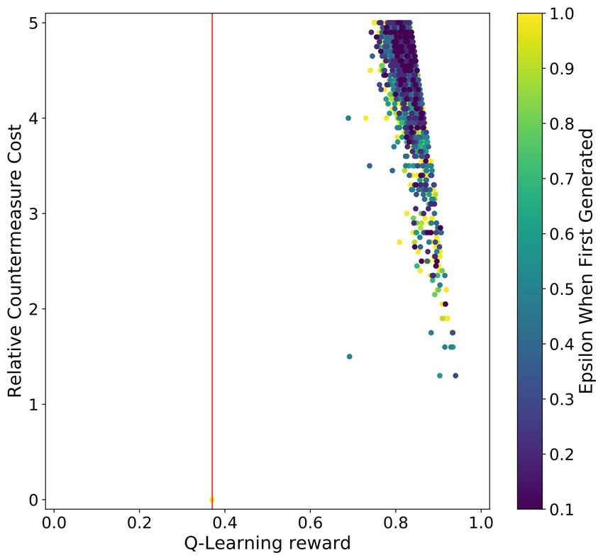
3

based SCA is difficult to succeed. Although the random search can reach similar
goals, we argue that our SCA-optimized reinforcement learning method can con-
sistently evolve the countermeasure selection, thus outputs reliable results. We
emphasize that we simulate the countermeasures to assess their influence on a
dataset. This is why we concentrate on hiding countermeasures, as it is easier
to simulate hiding than masking (and there are also more options, making the
selection more challenging). As we attack datasets that are already protected
with masking, we consider both countermeasure categories covered. What we
provide is an additional layer of resilience besides the masking countermeasure.
The optimized combinations of countermeasures work in both amplitude and
time domains and could be easily implemented in real-world targets. From a de-
veloper’s perspective, the optimized combination can become the development
guideline of protection mechanisms. In this paper, we conduct experiments with
results indicating the time-based countermeasures as the key ingredient of strong
resilience against deep learning-based SCA. Our main contributions are:
 1. We propose a novel reinforcement learning approach to construct low-cost
     hiding countermeasure combinations, making deep learning-based SCA dif-
     ficult to succeed.
 2. We motivate and develop custom reward functions for countermeasure se-
     lection to increase the SCA resilience.
 3. We conduct extensive experimental analysis considering four countermea-
     sures, two datasets, and two leakage models.
 4. We report on a number of countermeasures that indicate strong resilience
     against the selected profiling SCAs.
We plan to release our source code upon the acceptance of the paper (source
code is available through program chairs if required).

2     Preliminaries

Calligraphic letters (X ) denote sets and the corresponding upper-case letters
(X) random variables and random vectors X over X . The corresponding lower-
case letters x and x denote realizations of X and X, respectively. A dataset T is
a collection of traces (measurements). Each trace ti is associated with an input
value (plaintext or ciphertext) di and a key candidate ki . Here, k ∈ K and k ∗
represents the correct key. As common in profiling SCA, we divide the dataset
into three parts: a profiling set of N traces, a validation set of V traces, and an
attack set of Q traces.

2.1   Deep Learning and Profiling Side-channel Analysis

We consider the supervised learning task where the goal is to learn a func-
tion f that maps an input to the output (f : X → Y )) based on examples
of input-output pairs. There is a natural mapping between supervised learning
and profiling SCA. Supervised learning has two phases: training and test. The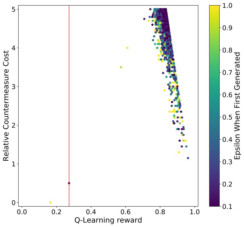
4

training phase corresponds to the SCA profiling phase, and the testing phase
corresponds to the side-channel attack phase. The profiling SCA runs under the
following setup:
  – The goal of the profiling phase is to learn the parameters of the profiling
     model minimizing the empirical risk represented by a loss function on a
     profiling set of size N .
  – The goal of the attack phase is to make predictions about the classes
     y(x1 , k ∗ ), . . . , y(xQ , k ∗ ), where k ∗ represents the secret (unknown) key on
     the device under the attack.
    Probabilistic deep learning algorithms output a matrix that denotes the prob-
ability that a certain measurement should be classified into a specific class. Thus,
the result is a matrix P with dimensions equal to Q × c, where c denotes the
number of output labels (classes). The probability S(k) for any key candidate k
is the maximum log-likelihood distinguisher:
                                          Q
                                          X
                                 S(k) =         log(pi,v ).                            (1)
                                          i=1

The value pi,v represents the probability that a specific class v is predicted. The
class v is obtained from the key and input through a cryptographic function and
a leakage model.
    From the matrix P , it is straightforward to obtain the accuracy of the model
f . Still, in SCA, an adversary is not interested in predicting the classes in the
attack phase but in obtaining the secret key k ∗ . Thus, to estimate the difficulty of
breaking the target, it is common to use metrics like guessing entropy (GE) [21].
    Given Q traces in the attack phase, an attack outputs a key guessing vector
g = [g1 , g2 , . . . , g|K| ] in decreasing order of probability (g1 is the most likely key
candidate and g|K| the least likely key candidate). Guessing entropy represents
the average position of k ∗ in g.

2.2   Side-channel Countermeasures

It is common to protect the implementation with countermeasures. Countermea-
sures aim to break the statistical link between intermediate values and traces
(e.g., power consumption or EM emanation). There are two main categories of
countermeasures for SCA: masking and hiding.
     In masking, a random mask is generated to conceal every intermediate value.
More precisely, random masks are used to remove the correlation between the
measurements and the secret data. In general, there are two types of masking:
Boolean masking and arithmetic masking.
     On the other hand, the goal of hiding is to make measurements looking ran-
dom or constant. Hiding decreases the signal-to-noise ratio (SNR) only. Hiding
can happen in the amplitude (e.g., adding noise) and time (e.g., desynchroniza-
tion, random delay interrupts, jitter) dimensions. In our work, we simulate only
hiding countermeasures as masking is always active.
5

2.3   Datasets and Leakage Models

The two datasets we use are versions of the ASCAD database [2]. Both datasets
contain the measurements from an 8-bit AVR microcontroller running a masked
AES-128 implementation. We attack the first masked key byte (key byte three).
The datasets are available at https://github.com/ANSSI-FR/ASCAD. The first
dataset version has a fixed key (thus, the key is the same in the profiling and
attack set). This dataset consists of 50 000 traces for profiling and 10 000 for the
attack. From 50 000 traces in the profiling set, we use 45 000 traces for profiling
and 5 000 for validation. Each trace has 700 features (preselected window). The
second version has random keys, with 200 000 traces for profiling and 100 000 for
the attack. We use 5 000 traces from the attack set for validation (note that the
attack set has a fixed but a different key from the profiling set). Each trace has
1 400 features (preselected window).

We consider two leakage models:
 – The Hamming weight (HW) leakage model - the attacker assumes the leakage
   proportional to the sensitive variable’s Hamming weight. Considering the
   AES cipher with 8-bit S-boxes, this leakage model has nine classes for a
   single key byte (values from 0 to 8).
 – The Identity (ID) leakage model - the attacker considers the leakage in the
   form of an intermediate value of the cipher. Considering the AES cipher with
   8-bit S-boxes, this leakage model results in 256 classes for a single key byte
   (values from 0 to 255).

2.4   Reinforcement Learning

Reinforcement learning (RL) aims to teach an agent how to perform a task by
letting the agent experiment and experience the environment. There are two
main categories of reinforcement learning algorithms: policy-based algorithms
and value-based algorithms. Policy-based algorithms directly try to find this
optimal policy. Value-based algorithms, however, try to approximate or find the
value function that assigns state-action pairs a reward value. Most reinforcement
learning algorithms are centered around estimating value functions, but this is
not a strict requirement for reinforcement learning. For example, methods such
as genetic algorithms or simulated annealing can all be used for reinforcement
learning without ever estimating value functions [22]. In this research, we only
focus on Q-Learning, belonging to the value estimation category.
    Reinforcement learning has fundamental differences compared with super-
vised and unsupervised machine learning, commonly adopted by the SCA com-
munity. Supervised machine learning learns from a set of examples (input-output
pairs) labeled with the correct answers. A benefit of reinforcement learning over
supervised machine learning is that the reward signal can be constructed with-
out prior knowledge of the correct course of action, which is especially useful
if such a dataset does not exist or is infeasible to obtain. In unsupervised ma-
chine learning, the algorithm attempts to find some (hidden) structure within a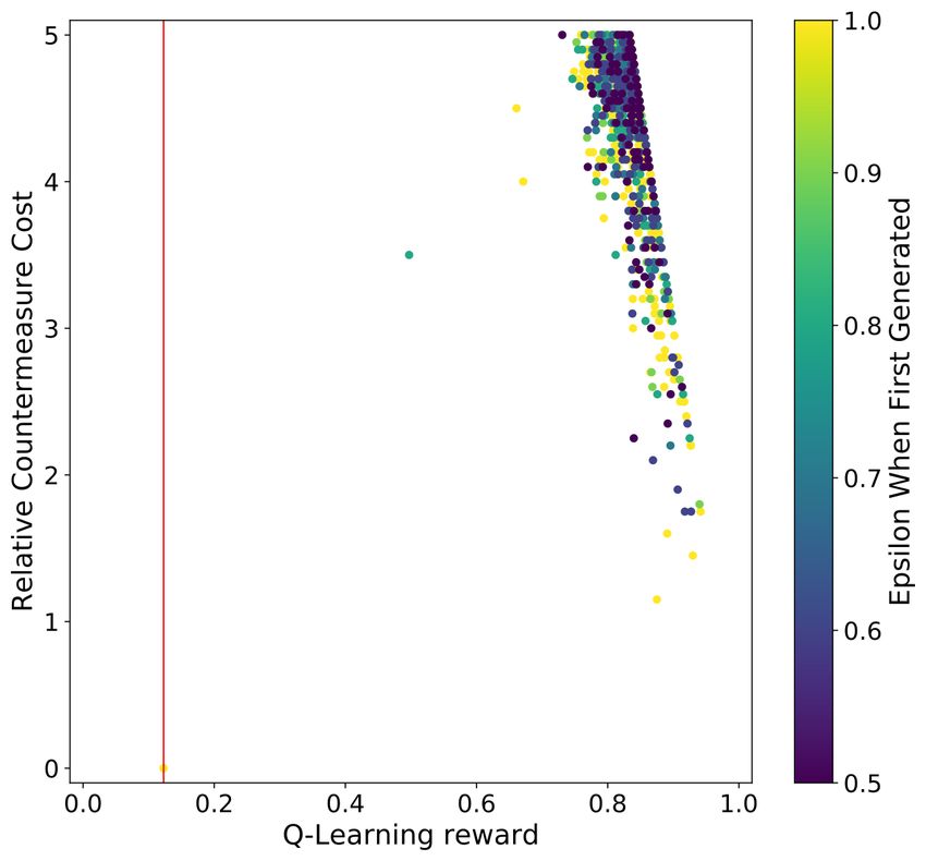
6

dataset, while reinforcement learning aims to teach an agent how to perform a
task through rewards and experiments [22].

Q-Learning Q-Learning was introduced in 1989 by Chris Watkins [23] with
an aim not only to learn from the outcome of a set of state-action transitions
but from each of them individually. Q-learning is a value-based algorithm that
tries to estimate q∗ (s, a), the reward of taking action a in the state s under
the optimal policy, by iteratively updating its stored q-value estimations using
Eq. (2). The simplest form of Q-learning stores these q-value estimations as a
simple lookup table and initializes them with some chosen value or method. This
form of Q-learning is also called Tabular Q-learning.
    Eq. (2) is used to incorporate the obtained reward into the saved reward
for the current state Rt . St and At are the state and action at time t, and
Q(St , At ) is the current expected reward for taking action At in state St . α
and γ are the q-learning rate and discount factor, which are hyperparameters
of the Q-learning algorithm. The q-learning rate determines how quickly new
information is learned, while the discount factor determines how much value to
assign to short-term versus long-term rewards. Rt+1 is the currently observed
reward for having taken action At in state St . maxa Q(St+1 , a) is the maximum
of the expected reward of all the actions a that can be taken in state St+1 .

                                   h                                      i
      Q(St , At ) ← Q(St , At ) + α Rt+1 + γ max Q(St+1 , a) − Q(St , At ) .   (2)
                                              a

3   Related Works
We divide related works into two directions: improving deep learning-based SCA
and improving the defenses against such attacks. In the first direction, from
2016 and the first paper using convolutional neural networks [11], there are
continuous improvements in the attack performance. Commonly, such works
investigate (note this is only a small selection of the papers):
  – the importance of hyperparameters and designing top-performing
    neural networks. Benadjila et al. made an empirical evaluation of different
    CNN hyperparameters for the ASCAD dataset [2]. Perin and Picek explored
    the various optimizer choices for deep learning-based SCA [15]. Zaid et al.
    proposed a methodology to select hyperparameters related to the size of
    layers in CNNs [29]. To the best of our knowledge, this is the first method-
    ology to build CNNs for SCA. Wouters et al. [24] improved upon the work
    from Zaid et al. [29] and showed it is possible to reach similar attack per-
    formance with significantly smaller neural network architectures. Wu et al.
    used Bayesian optimization to find optimal hyperparameters for multilayer
    perceptron and convolutional neural network architectures [25]. Rijsdijk et
    al. used reinforcement learning to design CNNs that exhibit strong attack
    performance and have a small number of trainable parameters [20]. Our re-
    inforcement learning setup is inspired by the one presented here, especially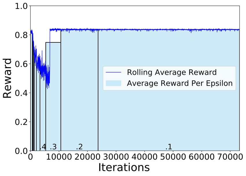
7

    the reward function part 1 To improve the attack performance, some authors
    also proposed custom elements for neural networks for SCA. For instance,
    Zaid et al. [28], and Zhang et al. [30] introduced new loss functions that
    improve the attack performance.
  – well-known techniques from the machine learning domain to im-
    prove the performance of deep learning-based attacks. Cagli et al.
    showed how CNNs could defeat jitter countermeasure, and they used data
    augmentation to improve the attack process [3]. Kim et al. constructed VGG-
    like architecture that performs well over several datasets, and they use regu-
    larization in the form of noise added to the input [10]. Perin et al. showed how
    ensembles could improve the attack performance even when single models
    are only moderately successful [14]. Wu et al. used the denoising autoen-
    coder to remove the countermeasures from measurements to improve the
    attack performance [26]. Perin et al. considered the pruning technique and
    the lottery ticket hypothesis to make small neural networks reach top attack
    performance [16].
  – explainability and interpretability of results. Hettwer et al. investi-
    gated how to select points of interest for deep learning by using three deep
    neural network attribution methods [8]. Masure et al. used gradient visual-
    ization to discover where the sensitive information leaks [12].
    On the other hand, the domain of countermeasures’ design against machine
learning-based SCA is much less explored 2 . Indeed, to the best of our knowledge,
there are only a few works considering this perspective as briefly discussed in
Section 1. At the same time, it is unclear how such countermeasures would be
implemented or the implementation cost.

4     The RL-based Countermeasure Selection Framework
4.1     General Setup
We propose a Tabular Q-Learning algorithm based on MetaQNN that can se-
lect countermeasures, including their parameters, to simulate their effectiveness
on an existing dataset against an arbitrary neural network. To evaluate the ef-
fectiveness of the countermeasures, we use guessing entropy. There are several
aspects to consider if using MetaQNN:
 1. We need to develop an appropriate reward function that considers particu-
    larities of the SCA domain. Thus, considering only machine learning metrics
    would not suffice.
 2. MetaQNN uses a fixed α (learning rate) for Q-Learning while using a learn-
    ing rate schedule where α decreases either linearly or polynomially are the
    normal practice [6].
1
    The authors mention they conducted a large number of experiments to find a reward
    function that works well for different datasets and leakage models, so we decided to
    use the same reward function.
2
    Many works consider the development of SCA countermeasures, but not specifically
    against deep learning approaches.
8

 3. One of the shortcomings of MetaQNN is that it requires significant compu-
    tational power and time to explore the search space properly. As we consider
    several different countermeasures with its hyperparameters, this results in a
    very large search space.
    We model the selection of the right countermeasures and their parameters as a
Markov Decision Process (MDP). Specifically, each state has a transition towards
an accepting state with the currently selected countermeasures. Each counter-
measure can only be applied once per Q-Learning iteration, so the resulting set
of chosen countermeasures can be empty (no countermeasure being added) or
contain up to four different countermeasures in any order.3 One may consider
that with the larger number of countermeasures being added to the traces, the
more difficult the secret information to be retrieved by the side-channel attacks.
However, one should note that the implementation of the countermeasure is not
without any cost. Indeed, some software-based countermeasures add overhead in
the execution efficiency (i.e., dummy executions), while others add overhead in
total power consumption (i.e., dedicated noise engine).
    To select optimal countermeasure combinations with a limited burden on the
device, a cost function that can approximate the implementation costs should
balance the strength of the countermeasure implementation and the security of
the device. Thus, such a function is also a perfect candidate as a reward function
to guide the Q-learning process. While we try to base the costs on real-world
implications of adding each of the countermeasures in a chosen configuration,
translating the total cost back to a real-world metric is nontrivial. Therefore,
we design a cost function associated with each countermeasure, where the value
depends on the chosen countermeasure’s configuration. The total cost of the
countermeasure set, ctotal , is defined as:
                                              |C|
                                              X
                                   ctotal =         ci .                         (3)
                                              i=1

    Here, C represents the set of applied countermeasures, and ci is the cost
of the individual countermeasure defined differently for each countermeasure.
Based on the values chosen by Wu et al. [26] for the ASCAD fixed key dataset,
we set the total cost budget cmax to five, but it can be easily adjusted for other
implementations. cmax set the upper limit of the applied countermeasure so that
the selected countermeasure is in a reasonable range and avoid the algorithm to
’cheat’ by adding all possible countermeasures with the strongest settings. Only
countermeasure configurations within the remaining budget are selectable by
the Q-Learning agent. If the countermeasures successfully defeat the attack (GE
does not reach 0 within the configured number of attack traces), any leftover
budget is used as a component of the reward function. By evaluating the reward
function, we can find the best budget-effective countermeasure combinations,
3
    The countermeasures set is an ordered set based on the order that the RL agent
    selected them. Since the countermeasures are applied in this order, sets with the
    same countermeasures but a different ordering are treated as disjoint.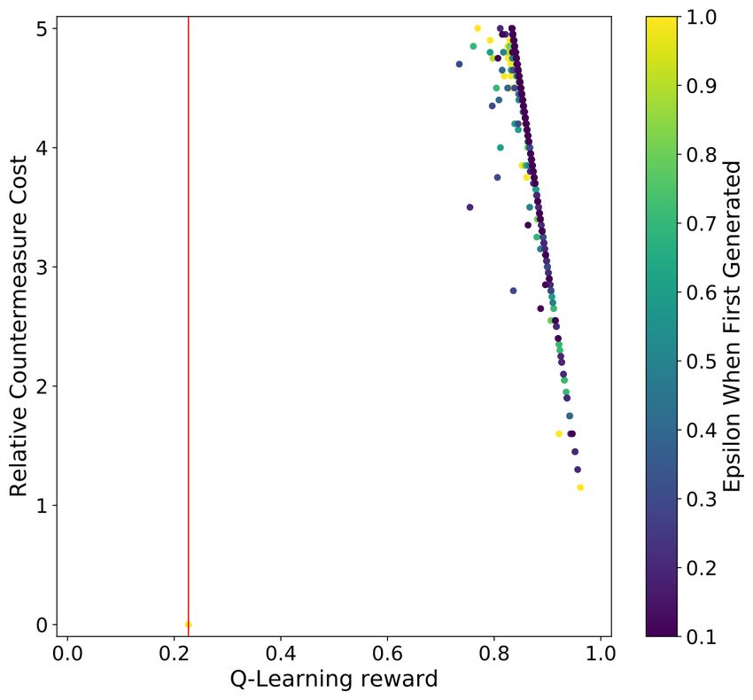
9

together with their settings, to protect the device from the SCA with the lowest
budget.
    We evaluated four countermeasures: desynchronization, uniform noise, clock
jitter, and random delay interrupt (RDI), and applied them to the original
dataset. The performance of each countermeasure against deep learning-based
SCA can be found in [26]. The countermeasures are all applied a-posteriori to
the chosen dataset in our experiments. Note that the implementations of the
countermeasure are based on the countermeasure designs from Wu et al. [26].
Already that work showed that a combination of countermeasures makes the
attack more difficult to succeed.
    Some of these countermeasures generate traces of varying length. To make
them all of the same length, the traces shorter than the original are padded with
zeroes, while any longer traces are truncated back to the original length. The
detailed implementation and design of each countermeasure’s cost function are
discussed in the following sections. We emphasize that the following definitions
of the countermeasure cost are customized for the selected attack datasets. They
can be easily tuned and adjusted to other implementations based on the actual
design specifications.

Desynchronization We draw a number uniformly between 0 and the chosen
maximum desynchronization for each trace in the dataset and shift the trace by
that number of features. In terms of the cost for desynchronization, Wu et al.
showed that a maximum desynchronization of 50 greatly increases the attack’s
difficulty. This leads us to set the desynchronization level (desync level) ranges
from 5 to 50 in a step of 5 (thus, not allowing the desynchronization value so large
that it will be trivial to defeat the deep learning attack). The cost calculation for
desynchronization is defined in Eq. (4). Note that the maximum cdesync is five,
which matches the cmax we defined as the total cost of countermeasures (which
is why cdesync needs to be divided by ten).
                                         desync level
                             cdesync =                .                          (4)
                                             10

Uniform noise Several sources, such as the transistor, data buses, the trans-
mission line to the record devices such as oscilloscopes, or even the work environ-
ment, introduce noise to the amplitude domain. Adding uniform noise amounts
to adding a uniformly distributed random value to each feature. To make sure
the addition of the noise causes a similar effect on different datasets, we set the
maximum noise level based on the dataset variation defined by Eq. (5):
                                               p
                                                  V ar(T )
                          max noise level =                .                    (5)
                                                    2
    Here, T denotes the measured leakage traces. Then, max noise level is mul-
tiplied with a noise f actor parameter, ranging from 0.1 to 1.0 with steps of 0.1,
to control the actual noise level introduced to the traces. Since the noise f actor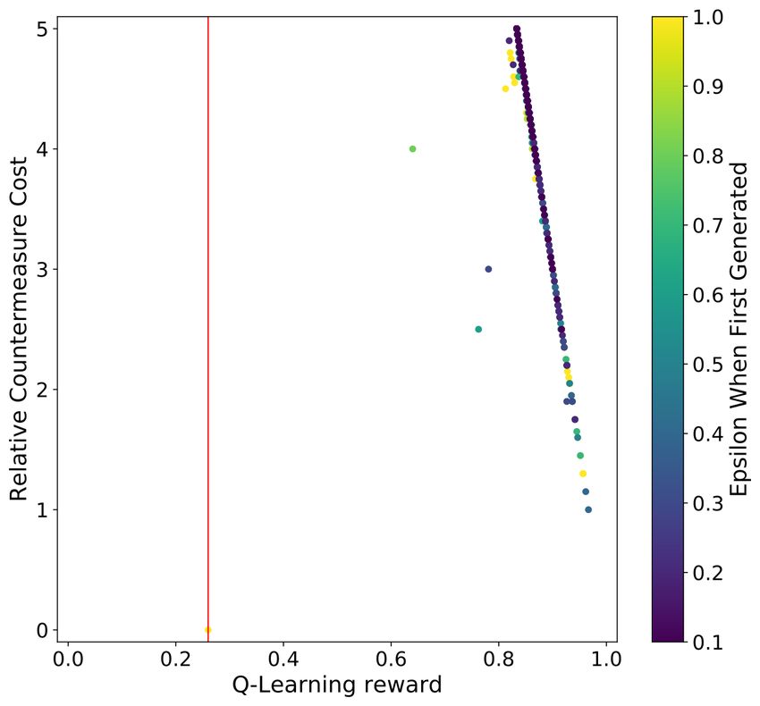
10

is the only adjustable parameter, we define the cost of the uniform noise in
Eq. (6) to make sure that the the maximum cnoise equals to cmax .

                           cnoise = noise f actor × 5.                         (6)

Clock Jitter One way of implementing clock jitters is by introducing the insta-
bility in the clock [3]. While desynchronization introduces randomness globally
in the time domain, the introduction of clock jitters increases each sampling
point’s randomness, thus increasing the alignment difficulties. When applying
the clock jitter countermeasure to the ASCAD dataset, Wu et al. chose eight as
the jitter level, but none of the attacks managed to retrieve the key in 10 000
traces.Thus, we decide to tune the jitter level (jitter level) with a maximum
of eight. The corresponding cost function is defined in Eq. 7. In the following
experiments, we set the jitter level ranging from 2 to 8 in a step of 2. Again,
maximum cjitter value matches the cmax value we defined before.

                           cjitter = jitter level × 1.6.                       (7)

Random Delay Interrupts (RDIs) Similar to clock jitter, RDIs introduce
local desynchronization in the traces. We implement RDIs based on the floating
mean method [5]. More specifically, we add RDI for each feature in each trace
with a configurable probability. If an RDI occurs for a trace feature, we select
the delay length based on the A and B parameters, where A is the maximum
length of the delay and B is a number 6 A. Since RDIs in practice are imple-
mented using instructions such as nop, we do not simply flatten the simulated
power consumption but introduce peaks with a configurable amplitude. Since
the RDI countermeasure has many adjustable parameters, it will, by far, have
the most MDP paths dedicated to it, meaning that during random exploration,
it is far more likely to select it as a countermeasure. To offset this, we reduce
the number of configurable parameters by fixing the amplitude for RDIs based
on the max noise level defined in Eq. 5 for each dataset. Furthermore, we add
1 to the cost of any random delay interrupt countermeasure, as shown in Eq. 8,
defining the cost function for RDIs.

                                  3 × probability × (A + B)
                     crdi = 1 +                             ,                  (8)
                                              2
where A ranges from 1 to 10, B ranges from 0 to 9, and probability ranges from
0.1 to 1 in a step of 1. We emphasize that we made sure the selected B value is
never larger than A.
    When looking at the parameters Wu et al. [26] used for random delay inter-
rupts applied on the ASCAD fixed key dataset, A = 5, B = 3 and probability =
0.5, none of the chosen attack methods show any signs of converging on the cor-
rect key guess, even after 10 000 traces. With our chosen crdi , this configuration
cost equals seven, which we consider appropriate.
11
We emphasize that we selected the ranges for each countermeasure based on
the related works, while the cost of such countermeasures is adjusted based on the
maximum allowed budget. While these values are indeed arbitrary, they can be
easily adjusted for any real-world setting. We do not give to each countermeasure
the same cost, but normalize it so that the highest value for each countermeasure
represents a setting that is difficult to break and consumes the whole cost budget.
4.2 Reward Functions
To allow MetaQNN to be used for the countermeasure selection, we use a rela-
tively complex reward function. This reward function incorporates the guessing
entropy and is composed of four metrics: 1) t0 : the percentage of traces required
0
to get the GE to 0 out of the fixed maximum attack set size; 2) GE10 : the GE
0
value using 10% of the attack traces; 3) GE50 : the GE value using 50% of the
attack traces and 4) c0 : the percentage of countermeasures budget left over out
of the fixed maximum budget parameter. The formal definitions of the first three
metrics are expressed in Eqs. (9), (10), (11), and (12). We note this is the same
reward function as used in [20].
tmax − min(tmax , QtGE )
t0 = . (9)
tmax
0 128 − min(GE10 , 128)
GE10 = . (10)
128
0 128 − min(GE50 , 128)
GE50 = . (11)
128
cmax − ctotal
c0 = . (12)
cmax
The first three metrics of the reward function are derived from the GE metric,
aiming to reward neural network architectures based on their attack performance
using the configured number of attack traces.4 Since we reward countermeasure
sets that manage to reduce the SCA performance, we incorporate the inverse of
these metrics into our reward functions, as these metrics are appropriate in a
similar setting [20]. Combining these three metrics allows us to assess the coun-
termeasure set performance, even if the neural network model does not retrieve
the secret key within the maximum number of attack traces. We incorporate
these metrics inversely into our reward function by subtracting their value from
their maximum value. Combined, the sum of the maximum values from which
we subtract (multiplied by their weight in the reward function) equals 2.5, as
4
Note that the misleading GE behavior as discussed in [27] may happen during the
experiments. Although one could reverse the ranking provided by an attack to obtain
the correct key, we argue it is not possible in reality as an attacker would always
assume the correct key being the one with the lowest GE (most likely guess).12
shown in Eq. (13). The weight of each metric is determined based on a large
number of experiments.
In terms of the fourth metric c0 , recall C is the set of countermeasures cho-
sen by the agent, and ctotal equals five. We only apply this reward when the
key retrieval is unsuccessful in tmax traces, as we do not want to reward small
countermeasure sets for their size if they do not adequately decrease the attack
performance. Combining these four metrics, we define the reward function as in
Eq. (13), which gives us a total reward between 0 and 1. To better reward the
countermeasure set performance, making the SCA neural networks require more
0
traces for a successful break, a smaller weight is set on GE50 .
(
1 2.5 − t0 − GE10
0 0
− 0.5 × GE50 , if tGE=0 < tmax
R= × 0 0 0
(13)
3 2.5 − GE10 − 0.5 × GE50 + 0.5 × c , otherwise
We multiply the entire set of metrics by 31 to normalize our reward function
between 0 and 1. While this reward function does look complicated, it is derived
based on the results from [20] and our experimental tuning lasting several weeks.
Still, we do not claim the presented reward function is optimal, but it gives good
results. Further improvements are always possible, especially from the budget
perspective or the cost of a specific countermeasure.
5 Experimental Results
To assess the performance of the selected set of countermeasures for each dataset
and leakage model, we perform experiments with different CNN models (as those
are reported to reach top results in SCA, see, e.g. [10,29]). Those models are
tuned for each dataset and leakage model combination without considering hid-
ing countermeasures that we simulate. One could consider this not to be fair
as those architectures do not necessarily work well with countermeasures. Still,
there are two reasons to follow this approach as we 1) do not know a priori the
best set of countermeasures and we do not want to optimize both architectures
and countermeasures at the same time, and 2) evaluate against state-of-the-art
architectures that are not tuned against any of those countermeasures to allow
a fair assessment of all architectures.
Specifically, we use reinforcement learning to select the model’s hyperparam-
eter [20]. We execute the search algorithm for every dataset and leakage model
combination and select the top-performing models over 2 500 iterations. To assess
the performance of the Q-Learning agent, we compare the average rewards per ε.
For instance, a ε of 1.0 means the network was generated completely randomly,
while an ε of 0.1 means that the network was generated while choosing random
actions 10% of the time. For the test setup, we use an NVIDIA GTX 1080 Ti
graphics processing unit (GPU) with 11 Gigabytes of GPU memory and 3 584
GPU cores. All of the experiments are implemented with the TensorFlow [1]
computing framework and Keras deep learning framework [4].13
The details about the specific architectures can be found in Table 1. Note
that Rijsdijk et al. implemented two reward functions: one that only consid-
ers the attack performance, and the other that also considers the network size
(small reward function) [20]. We consider both reward functions aligned with
that paper, leading to two models used for testing; the one denoted with RS
is the model optimized with the small reward function. For all models, we use
he unif orm and selu as kernel initializer and activation function.
Test models Convolution Pooling Fully-connected layer
(filter number, size) (size, stride)
ASCADHW Conv(16,100) avg(25,25) 15+4+4
ASCADHW RS Conv(2,25) avg(4,4) 15+10+4
ASCADID Conv(128,25) avg(25,25) 20+15
ASCADID RS Conv(2+2+8, 75+3+2) avg(25+4+2, 25+4+2) 10+4+2
ASCAD RHW Conv(4, 50) avg(25, 25) 30+30+30
ASCAD RHW RS Conv(8, 3) avg(25, 25) 30+30+20
ASCAD RID Conv(128, 3) avg(75, 75) 30+2
ASCAD RID RS Conv(4, 1) avg(100, 75) 30+10+2
Table 1: CNN architectures used in the experiments [20].
5.1 ASCAD Fixed Key Dataset
Figure 1 shows the scatter plot results for the HW and ID leakage models for
both the regular and RS CNN. The vertical red line indicates the highest Q-
learning reward for the countermeasure set, which could not prevent the CNN
from retrieving the key within the configured 2 000 attack traces. Notably, a
sharp line can be found on the right side of the Q-Learning reward plots, which
is solely due to the c0 component of the reward function. Although the selected
CNNs can retrieve the secret key when no countermeasures were applied (c0 =
0) for all experiments with both HW and ID leakage models, as soon as any
countermeasure is applied, the attack becomes unsuccessful with 2 000 attack
traces. Indeed, we observe that only very few countermeasures seem inefficient
in defeating the deep learning attacks from the result plots.
For the experiments presented, the top countermeasures for ASCAD using
different profiling models are listed in Table 2. Notably, the best countermeasure
set in terms of performance and cost for this CNN consists of desynchronization
with a level equal to ten, which could be caused by the lack of sufficient convolu-
tion layers (only one) in countering such a countermeasure. The rest of the top
20 countermeasure sets include or solely consist of random delay interrupts. This
observation is also applied to other profiling models and ID leakage models. The
amplitude for RDI is fixed for each dataset, as explained in Section 4.1. In terms14
of the parameters of RDIs, B stays zero for all three profiling models, indicating
that A solely determines the length of RDIs. Indeed, B varies the mean of the
number of added RDIs and enhances the difficulties in learning from the data.
However, a larger B value would also increase the countermeasure cost, which is
against the reward function’s principle. From Table 2, we can observe both low
values of A and probability being applied to the RDIs countermeasure, indicating
the success of our framework in finding countermeasure with high performance
and low cost.
(a) ASCAD fixed key HW leakage (b) ASCAD fixed key ID leakage
model (192 hours). model (204 hours).
(c) ASCAD fixed key HW leakage (d) ASCAD fixed key ID leakage
model (RS) (196 hours). model (RS) (198 hours).
Fig. 1: An overview of the countermeasure cost, reward, and the ε value a coun-
termeasure combination set was first generated for the ASCAD with fixed key
dataset experiments. The red lines indicate the countermeasure set with the
highest reward for that GE reached 0 within 2 000 traces.
Next, we compare the general performance of the countermeasure sets be-
tween CNNs designed for the HW and ID leakage model. We observe that the
ID model appears to be at least a little better at handling countermeasures.15
Model Reward Countermeasures c0
ASCADHW 0.967 Desync(desync level=10) 1.00
ASCADHW RS 0.962 RDI(A=1,B=0,probability=0.10,amplitude=12.88) 1.15
ASCADID 0.957 RDI(A=2,B=0,probability=0.10,amplitude=12.88) 1.30
ASCADID RS 0.962 RDI(A=1,B=0,probability=0.10,amplitude=12.88) 1.15
Table 2: Best performing countermeasures for the ASCAD fixed key dataset.
Specifically, for the ID leakage model CNNs, the countermeasures’ Q-Learning
reward variance is higher, indicating that the ID model CNNs can better handle
countermeasures, making the countermeasure selection more important. This
observation is confirmed by the c0 value listed in Table 2: to reach a similar level
of the reward value, the countermeasures are implemented with a greater cost.
Considering the time required to run the reinforcement learning, we observe
we require around 200 hours on average, which is double the time required by
Rijsdijk et al. when finding neural networks that perform well [20]. In Figure 2,
we show the rolling average of the Q-learning reward and the average Q-learning
reward per epsilon for the ASCAD fixed key dataset. As can be seen, the reward
value for countermeasure gradually increases when more iteration is performed,
indicating that the agent is learning from the environment and becoming more
capable of finding effective countermeasure settings with a low cost. Then, the
reward value is saturated when ε reaches 0.1, meaning that the agent is well
trained and constantly finds well-performing countermeasures. One may notice
that the number of iterations performed is significantly higher than the config-
ured 1 700 iterations. This is because we only count an iteration when generating
a countermeasure set that was not generated before.
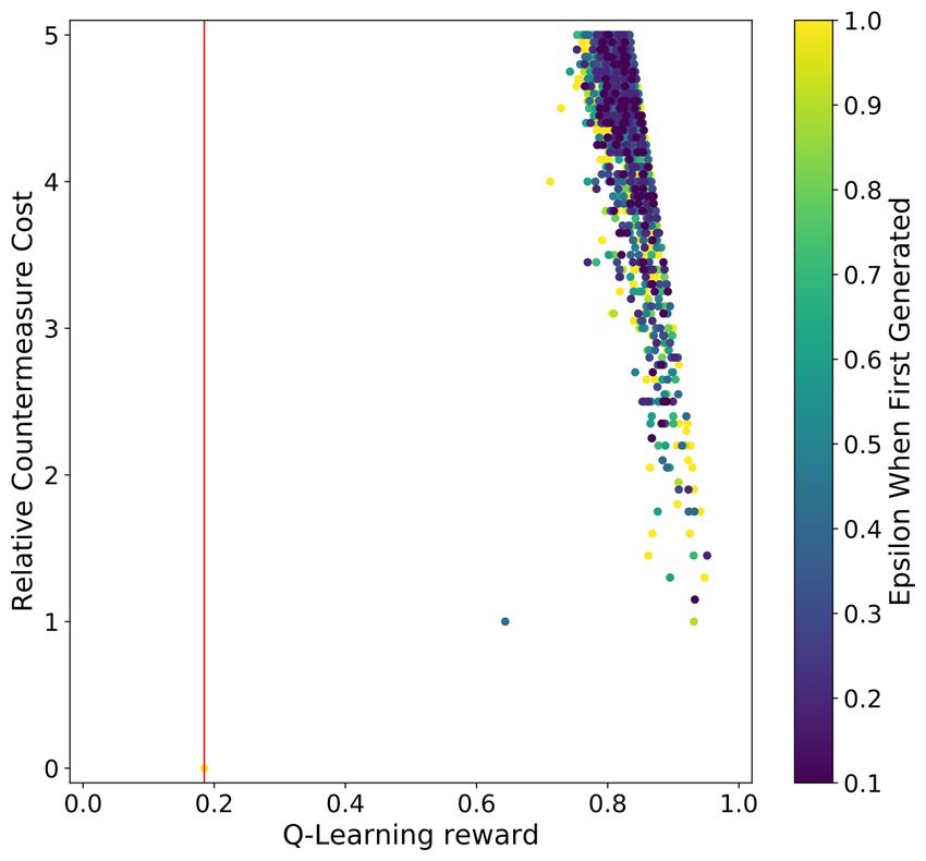
5.2 ASCAD Random Keys Dataset
The scatter plot results for both the HW and ID model for both the regular
and RS CNN are listed in Figure 3. Aligned with the ASCAD fixed key dataset
observation, the vertical red line in the plots is far away from the dots in the plot,
indicating that the countermeasure’s addition effectively increases side-channel
attack difficulty. Furthermore, we again see the sharp line on the right side of the
Q-Learning reward, which is caused by the c0 component of the reward function.
Compared with the ASCAD results for both leakage models (Figure 1), we
see a greater variation of the individual countermeasure implementations: even
with the same countermeasure cost, a different combination of countermeasures
and their corresponding setting may lead to unpredictable reward values. Fortu-
nately, we see this tendency with the RL-based countermeasure selection scheme
and can better select the countermeasures’ implementation with a limited bud-
get. Finally, we observe that the later leakage model is more effective in defeating
the countermeasure when comparing the HW and ID leakage models. In other
words, to protect the essential execution that leaks the ID information, more16
(a) ASCAD fixed key HW leakage (b) ASCAD fixed key ID leakage
model. model.
Fig. 2: An overview of the Q-Learning performance for the ASCAD with fixed
key dataset experiments. The blue line indicates the rolling average of the Q-
Learning reward for 50 iterations, where at each iteration, we generate and
evaluate a countermeasure set. The bars in the graph indicate the average Q-
Learning reward for all countermeasure sets generated during that ε. The results
for RS experiments are similar.
effort may be required to implement countermeasures. The top-performing coun-
termeasures for different profiling models are listed in Table 3. From the results,
RDIs again become the most effective one among all of the considered counter-
measures. The RDI amplitude is fixed at 16.95 for this dataset, as explained in
Section 4.1.
Interestingly, the countermeasures are implemented with higher costs when
compared with the one used for ASCAD with a fixed key. The reason could be
that training with random keys traces enhances the generalization of the profiling
model. What is more, we also observe that we require significantly longer time to
run the reinforcement learning framework: on average, 300 hours, which is more
than 12 days of computations. Interestingly, we see an outlier with the ASCAD
random keys for the ID leakage model, where only 48 hours were needed for the
experiments.
Model Reward Countermeasures c0
ASCAD RHW 0.940 RDI(A=1,B=0,probability=0.20,amplitude=16.95) 1.30
ASCAD RHW RS 0.952 RDI(A=2,B=1,probability=0.10,amplitude=16.95) 1.45
ASCAD RID 0.942 RDI(A=5,B=0,probability=0.10,amplitude=16.95) 1.75
ASCAD RID RS 0.962 RDI(A=1,B=0,probability=0.10,amplitude=16.95) 1.15
Table 3: Best performing countermeasures for the ASCAD random keys dataset.
The rolling average of the Q-learning reward and the average Q-learning
reward per ε for the ASCAD random keys dataset are given in Figure 4, Ap-17
(a) ASCAD random keys HW (b) ASCAD random keys ID
leakage model (280 hours). leakage model (48 hours).
(c) ASCAD random keys HW (d) ASCAD random keys ID
leakage model (RS) (296 hours). leakage model (RS) (309 hours).
Fig. 3: An overview of the countermeasure cost, reward, and the ε value a coun-
termeasure combination set was first generated for the ASCAD with random
keys dataset experiments. The red lines indicates the countermeasure set with
the highest reward for that GE reached 0 within 2 000 traces.
pendix A. Interestingly, at the beginning of Figure 4a, there is a significant drop
in Q-learning reward, followed by a rapid increase in the ε update from 0.4 to 0.3.
A possible explanation could be that the model we used is powerful in defeat-
ing the selected countermeasures at the early learning stage. Still, the algorithm
managed to learn from each interaction, finally selecting powerful countermea-
sures. In contrast, selecting countermeasure to defeat ASCAD RID is an easy
task: the reward value reaches above 0.8 at the very beginning, and it stops
increasing regardless of the number of iterations. Since each test consumes 300
hours on average, we stopped the tests after around 3 000 iterations. There is a
similar performance for settings with the RS objective in the ASCAD with the
fixed key dataset: the RL algorithm is constantly learning. The highest reward
value is obtained when ε reaches the minimum.18
6 Conclusions and Future Work
This paper presents a novel approach to designing side-channel countermeasures
based on reinforcement learning. We consider four well-known types of counter-
measures (one in the amplitude domain and three in the time domain), and we
aim to find the best combinations of countermeasures within a specific budget.
We conduct experiments on two datasets and report a number of countermeasure
combinations providing significantly improved resilience against deep learning-
based SCA. Our experiments show that the best performing countermeasure
combinations use the random delay interrupt countermeasure, making it a natu-
ral choice for real-world implementations. While the specific cost for each coun-
termeasure was defined arbitrarily (as well as the total budget), we believe the
whole approach is easily transferable to settings with real-world targets.
The experiments performed currently take significantly longer than might
be necessary, as we generate a fixed number of unique countermeasure sets. In
contrast, the chance to generate a unique countermeasure set towards the end of
the experiments is significantly smaller (due to the lower ε). For future work, we
plan to explore how to detect this behavior. Additionally, we plan to consider
multilayer perceptron architectures and sets of countermeasures that work well
for different datasets and leakage models.
References
1. Abadi, M., Agarwal, A., Barham, P., Brevdo, E., Chen, Z., Citro, C., Corrado,
G.S., Davis, A., Dean, J., Devin, M., Ghemawat, S., Goodfellow, I., Harp, A.,
Irving, G., Isard, M., Jia, Y., Jozefowicz, R., Kaiser, L., Kudlur, M., Levenberg,
J., Mané, D., Monga, R., Moore, S., Murray, D., Olah, C., Schuster, M., Shlens, J.,
Steiner, B., Sutskever, I., Talwar, K., Tucker, P., Vanhoucke, V., Vasudevan, V.,
Viégas, F., Vinyals, O., Warden, P., Wattenberg, M., Wicke, M., Yu, Y., Zheng,
X.: TensorFlow: Large-scale machine learning on heterogeneous systems (2015),
http://tensorflow.org/, software available from tensorflow.org
2. Benadjila, R., Prouff, E., Strullu, R., Cagli, E., Dumas, C.: Deep learning for
side-channel analysis and introduction to ASCAD database. J. Cryptographic
Engineering 10(2), 163–188 (2020). https://doi.org/10.1007/s13389-019-00220-8,
https://doi.org/10.1007/s13389-019-00220-8
3. Cagli, E., Dumas, C., Prouff, E.: Convolutional neural networks with data aug-
mentation against jitter-based countermeasures. In: Fischer, W., Homma, N.
(eds.) Cryptographic Hardware and Embedded Systems – CHES 2017. pp. 45–68.
Springer International Publishing, Cham (2017)
4. Chollet, F., et al.: Keras. https://github.com/fchollet/keras (2015)
5. Coron, J., Kizhvatov, I.: An Efficient Method for Random Delay Generation in
Embedded Software. In: Cryptographic Hardware and Embedded Systems - CHES
2009, 11th International Workshop, Lausanne, Switzerland, September 6-9, 2009,
Proceedings. pp. 156–170 (2009)
6. Even-Dar, E., Mansour, Y.: Learning rates for q-learning. J. Mach. Learn. Res. 5,
1–25 (Dec 2004)
7. Gu, R., Wang, P., Zheng, M., Hu, H., Yu, N.: Adversarial attack based counter-
measures against deep learning side-channel attacks (2020)19
8. Hettwer, B., Gehrer, S., Güneysu, T.: Deep neural network attribution methods for
leakage analysis and symmetric key recovery. In: Paterson, K.G., Stebila, D. (eds.)
Selected Areas in Cryptography – SAC 2019. pp. 645–666. Springer International
Publishing, Cham (2020)
9. Inci, M.S., Eisenbarth, T., Sunar, B.: Deepcloak: Adversarial crafting as a defensive
measure to cloak processes. CoRR abs/1808.01352 (2018), http://arxiv.org/
abs/1808.01352
10. Kim, J., Picek, S., Heuser, A., Bhasin, S., Hanjalic, A.: Make some noise. unleashing
the power of convolutional neural networks for profiled side-channel analysis. IACR
Transactions on Cryptographic Hardware and Embedded Systems pp. 148–179
(2019)
11. Maghrebi, H., Portigliatti, T., Prouff, E.: Breaking cryptographic implementations
using deep learning techniques. In: International Conference on Security, Privacy,
and Applied Cryptography Engineering. pp. 3–26. Springer (2016)
12. Masure, L., Dumas, C., Prouff, E.: Gradient visualization for general char-
acterization in profiling attacks. In: Polian, I., Stöttinger, M. (eds.) Con-
structive Side-Channel Analysis and Secure Design - 10th International
Workshop, COSADE 2019, Darmstadt, Germany, April 3-5, 2019, Proceed-
ings. Lecture Notes in Computer Science, vol. 11421, pp. 145–167. Springer
(2019). https://doi.org/10.1007/978-3-030-16350-1 9, https://doi.org/10.1007/
978-3-030-16350-1_9
13. Ouytsel, C.B.V., Bronchain, O., Cassiers, G., Standaert, F.: How to fool a black
box machine learning based side-channel security evaluation. Cryptogr. Com-
mun. 13(4), 573–585 (2021). https://doi.org/10.1007/s12095-021-00479-x, https:
//doi.org/10.1007/s12095-021-00479-x
14. Perin, G., Chmielewski, L., Picek, S.: Strength in numbers: Improving gener-
alization with ensembles in machine learning-based profiled side-channel anal-
ysis. IACR Transactions on Cryptographic Hardware and Embedded Systems
2020(4), 337–364 (Aug 2020). https://doi.org/10.13154/tches.v2020.i4.337-364,
https://tches.iacr.org/index.php/TCHES/article/view/8686
15. Perin, G., Picek, S.: On the influence of optimizers in deep learning-based side-
channel analysis. In: Dunkelman, O., Jr., M.J.J., O’Flynn, C. (eds.) Selected
Areas in Cryptography - SAC 2020 - 27th International Conference, Halifax,
NS, Canada (Virtual Event), October 21-23, 2020, Revised Selected Papers.
Lecture Notes in Computer Science, vol. 12804, pp. 615–636. Springer (2020).
https://doi.org/10.1007/978-3-030-81652-0 24
16. Perin, G., Wu, L., Picek, S.: Gambling for success: The lottery ticket hypothesis
in deep learning-based sca. Cryptology ePrint Archive, Report 2021/197 (2021),
https://eprint.iacr.org/2021/197
17. Picek, S., Heuser, A., Jovic, A., Bhasin, S., Regazzoni, F.: The curse of class
imbalance and conflicting metrics with machine learning for side-channel evalu-
ations. IACR Transactions on Cryptographic Hardware and Embedded Systems
2019(1), 209–237 (Nov 2018). https://doi.org/10.13154/tches.v2019.i1.209-237,
https://tches.iacr.org/index.php/TCHES/article/view/7339
18. Picek, S., Jap, D., Bhasin, S.: Poster: When adversary becomes the guardian
– towards side-channel security with adversarial attacks. In: Proceedings of the
2019 ACM SIGSAC Conference on Computer and Communications Security. p.
2673–2675. CCS ’19, Association for Computing Machinery, New York, NY, USA
(2019). https://doi.org/10.1145/3319535.3363284
19. Ramezanpour, K., Ampadu, P., Diehl, W.: Scarl: Side-channel analysis with rein-
forcement learning on the ascon authenticated cipher (2020)20
20. Rijsdijk, J., Wu, L., Perin, G., Picek, S.: Reinforcement learning for hy-
perparameter tuning in deep learning-based side-channel analysis. IACR
Transactions on Cryptographic Hardware and Embedded Systems 2021(3),
677–707 (Jul 2021). https://doi.org/10.46586/tches.v2021.i3.677-707, https://
tches.iacr.org/index.php/TCHES/article/view/8989
21. Standaert, F.X., Malkin, T.G., Yung, M.: A unified framework for the analysis
of side-channel key recovery attacks. In: Joux, A. (ed.) Advances in Cryptology -
EUROCRYPT 2009. pp. 443–461. Springer Berlin Heidelberg, Berlin, Heidelberg
(2009)
22. Sutton, R.S., Barto, A.G.: Reinforcement Learning: An Introduction. MIT Press,
2 edn. (2018), http://incompleteideas.net/book/the-book.html
23. Watkins, C.J.C.H.: Learning from delayed rewards. Phd thesis, University of Cam-
bridge England (1989)
24. Wouters, L., Arribas, V., Gierlichs, B., Preneel, B.: Revisiting a method-
ology for efficient cnn architectures in profiling attacks. IACR Transac-
tions on Cryptographic Hardware and Embedded Systems 2020(3), 147–
168 (Jun 2020). https://doi.org/10.13154/tches.v2020.i3.147-168, https://tches.
iacr.org/index.php/TCHES/article/view/8586
25. Wu, L., Perin, G., Picek, S.: I choose you: Automated hyperparameter tuning
for deep learning-based side-channel analysis. Cryptology ePrint Archive, Report
2020/1293 (2020), https://eprint.iacr.org/2020/1293
26. Wu, L., Picek, S.: Remove some noise: On pre-processing of side-
channel measurements with autoencoders. IACR Transactions on Crypto-
graphic Hardware and Embedded Systems 2020(4), 389–415 (Aug 2020).
https://doi.org/10.13154/tches.v2020.i4.389-415, https://tches.iacr.org/
index.php/TCHES/article/view/8688
27. Wu, L., Weissbart, L., Krček, M., Li, H., Perin, G., Batina, L., Picek, S.: On the
attack evaluation and the generalization ability in profiling side-channel analysis.
Cryptology ePrint Archive, Report 2020/899 (2020), https://eprint.iacr.org/
2020/899
28. Zaid, G., Bossuet, L., Dassance, F., Habrard, A., Venelli, A.: Ranking
loss: Maximizing the success rate in deep learning side-channel analy-
sis. IACR Trans. Cryptogr. Hardw. Embed. Syst. 2021(1), 25–55 (2021).
https://doi.org/10.46586/tches.v2021.i1.25-55, https://doi.org/10.46586/
tches.v2021.i1.25-55
29. Zaid, G., Bossuet, L., Habrard, A., Venelli, A.: Methodology for effi-
cient cnn architectures in profiling attacks. IACR Transactions on Cryp-
tographic Hardware and Embedded Systems 2020(1), 1–36 (Nov 2019).
https://doi.org/10.13154/tches.v2020.i1.1-36, https://tches.iacr.org/index.
php/TCHES/article/view/8391
30. Zhang, J., Zheng, M., Nan, J., Hu, H., Yu, N.: A novel evaluation metric for
deep learning-based side channel analysis and its extended application to imbal-
anced data. IACR Transactions on Cryptographic Hardware and Embedded Sys-
tems 2020(3), 73–96 (Jun 2020). https://doi.org/10.13154/tches.v2020.i3.73-96,
https://tches.iacr.org/index.php/TCHES/article/view/858321
A Q-Learning Performance for the ASCAD with Random
Keys Dataset
(a) ASCAD random keys HW (b) ASCAD random keys ID
leakage model. leakage model.
Fig. 4: An overview of the Q-Learning performance for the ASCAD with the
random keys dataset experiments. The blue line indicates the rolling average of
the Q-Learning reward for 50 iterations, where at each iteration, we generate
and evaluate a countermeasure set. The bars in the graph indicate the average
Q-Learning reward for all countermeasure sets generated during that ε. The
results for RS experiments are similar.You can also read