Remote Sounding of the Atmospheres of Uranus and Neptune - Dane Steven Tice First Year Report
←
→
Page content transcription
If your browser does not render page correctly, please read the page content below
Remote Sounding of the Atmospheres
      of Uranus and Neptune

                 Dane Steven Tice

                  First Year Report

                   Lincoln College
      Atmospheric, Oceanic and Planetary Physics
                 University of Oxford

                     August 2010

                Word Count: ∼13,800
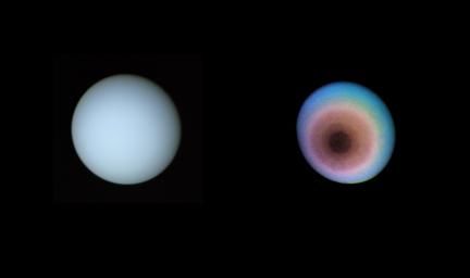
Abstract

Our solar system’s ‘ice giant’ planets, Uranus and Neptune, are unique among the planets
orbiting the Sun. Huge spheres of gas like all four giant planets, the ice giants possess
unique dynamics and properties which are derived from their cold temperatures and high
abundances of water and methane (CH4 ). Uranus’ large obliquity and extremely weak
internal heat source create a planet with dynamics controlled almost completely by solar
forcing. Neptune’s large inner heat flux and high water content create a planet with
intensely turbulent circulation and highly active storm features. This report describes the
techniques of remote sensing and retrieval theory as a means to study these fascinating
and unique bodies. A summary is provided of ice giant knowledge to date, relying on the
sparse collection of telescope and satellite data that has been analyzed. New telescope
data in the near-IR promises a means of further interpreting these planets, where no in
situ results have ever been obtained, and our knowledge is rudimentary. Preliminary
analysis of telescope data from NASA’s InfraRed Telescope Facility (IRTF) is presented,
and projections for future analysis are given.
Contents

1 Introduction                                                                            6

  1.1   Ice Giants: Uranus and Neptune . . . . . . . . . . . . . . . . . . . . . . . .    6

  1.2   Atmopsheric Observations of ‘Ice Giants’ . . . . . . . . . . . . . . . . . . .    7

2 Interpretation of Data                                                                  9

  2.1   Radiative Transfer and Planetary Spectra . . . . . . . . . . . . . . . . . .      9

  2.2   Retrieval Theory . . . . . . . . . . . . . . . . . . . . . . . . . . . . . . . . 13

  2.3   NEMESIS Overview . . . . . . . . . . . . . . . . . . . . . . . . . . . . . . 14

  2.4   Error Estimates and Retrieval Tuning . . . . . . . . . . . . . . . . . . . . . 17

  2.5   Model Efficiency and the Correlated-K Approximation . . . . . . . . . . . 18

3 Atmospheres of the Ice Giants                                                          22

  3.1   Brief Summary of Deep (Tropospheric) Composition . . . . . . . . . . . . . 22

  3.2   Temperature . . . . . . . . . . . . . . . . . . . . . . . . . . . . . . . . . . . 24

  3.3   Stratospheric Composition . . . . . . . . . . . . . . . . . . . . . . . . . . . 28

  3.4   Dynamics . . . . . . . . . . . . . . . . . . . . . . . . . . . . . . . . . . . . 32

                                            3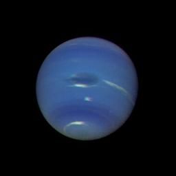
Contents                                                                                    4

        3.4.1   Thermal Forcing . . . . . . . . . . . . . . . . . . . . . . . . . . . . 32

        3.4.2   Zonal Structure . . . . . . . . . . . . . . . . . . . . . . . . . . . . . 33

        3.4.3   Vertical and Meridional Flow . . . . . . . . . . . . . . . . . . . . . 35

  3.5   Clouds and Hazes . . . . . . . . . . . . . . . . . . . . . . . . . . . . . . . . 37

        3.5.1   Uranus . . . . . . . . . . . . . . . . . . . . . . . . . . . . . . . . . . 37

        3.5.2   Neptune . . . . . . . . . . . . . . . . . . . . . . . . . . . . . . . . . 40

  3.6   Discrete Features . . . . . . . . . . . . . . . . . . . . . . . . . . . . . . . . 42

        3.6.1   Uranus . . . . . . . . . . . . . . . . . . . . . . . . . . . . . . . . . . 43

        3.6.2   Neptune . . . . . . . . . . . . . . . . . . . . . . . . . . . . . . . . . 45

  3.7   Variability . . . . . . . . . . . . . . . . . . . . . . . . . . . . . . . . . . . . 46

        3.7.1   Spatial Variability   . . . . . . . . . . . . . . . . . . . . . . . . . . . 47

        3.7.2   Temporal Variability . . . . . . . . . . . . . . . . . . . . . . . . . . 48

4 Results                                                                                  51

  4.1   IRTF Observations . . . . . . . . . . . . . . . . . . . . . . . . . . . . . . . 51

  4.2   Image Processing . . . . . . . . . . . . . . . . . . . . . . . . . . . . . . . . 52

        4.2.1   SpeXtool . . . . . . . . . . . . . . . . . . . . . . . . . . . . . . . . . 52

        4.2.2   Further Data Processing . . . . . . . . . . . . . . . . . . . . . . . . 55

        4.2.3   Solar Standards . . . . . . . . . . . . . . . . . . . . . . . . . . . . . 57

  4.3   Preliminary Retrievals . . . . . . . . . . . . . . . . . . . . . . . . . . . . . 57
Contents 5
5 Future Work 62
5.1 Data Processing . . . . . . . . . . . . . . . . . . . . . . . . . . . . . . . . . 62
5.1.1 Stellar Standard Analysis . . . . . . . . . . . . . . . . . . . . . . . 62
5.1.2 Air Mass . . . . . . . . . . . . . . . . . . . . . . . . . . . . . . . . . 63
5.2 Choosing a Focused Thesis Topic . . . . . . . . . . . . . . . . . . . . . . . 64
5.2.1 IRTF Data . . . . . . . . . . . . . . . . . . . . . . . . . . . . . . . 64
5.2.2 Other Available Data . . . . . . . . . . . . . . . . . . . . . . . . . . 65
5.2.3 Improved Methane Absorption Data . . . . . . . . . . . . . . . . . 66
5.3 Graduate Study Timeline . . . . . . . . . . . . . . . . . . . . . . . . . . . 66Chapter 1
Introduction
1.1 Ice Giants: Uranus and Neptune
Lying farthest from the Sun, our solar system’s ice ‘giant’ planets, Uranus and Neptune,
have been the least understood of the planets ever since man began studying the night
sky. While the existence of the classical planets, Mercury, Venus, Mars, Jupiter and
Saturn, has been known since ancient times, the first breakthroughs in understanding
these planets came from Galileo during the Scientific Revolution. Scientists have studied
those five planets avidly ever since Galileo first turned his telescope, which magnified only
about thirty times, towards the sky.
Because Uranus and Neptune are much smaller than the ‘gas giants’ Jupiter and Saturn,
and are positioned much farther from the Sun, they appear much less bright than the
classical planets. Despit advances in telescopic ability, it was not until 1781 that Uranus
was accidentally discovered by William Herschel. The analysis of observed perturbations
in Uranus’ orbit led astronomers to predict the presence of Neptune, a result confirmed
by Johann Gottfried Galle in 1846.
Once discovered, it was possible to determine some basic physical parameters of the ice
giants. Uranus and Neptune, are approximately 19 and 30 times farther from the Sun
than the Earth, respectively, have the longest planetary orbits in the solar system. Uranus
61.2. Atmopsheric Observations of ‘Ice Giants’ 7 spends 84 years circumnavigating the Sun, while Neptune completes its orbit in 165 years. The ice giants, like the gas giants, have no rocky surface, and are composed primarily of much lighter material than Earth. Uranus and Neptune are not as large or massive as Jupiter or Saturn, but they are much larger and more massive than Earth. Both have radii about 4 times the size of Earth’s, and masses about 15 and 17 times Earth’s, respectively. These values indicate the densities of Uranus and Neptune are 1.27 and 1.76 grams·cm-3 and that they are composed primarily of hydrogen, helium, and various ices, notably water and methane. Beyond this basic information, largely determined from simple calculations derived from Newtonian orbital dynamics, not much else is known due to the great distances involved in the outer solar system which continue to hamper efforts to study Uranus and Neptune. Telescope observations of these two planets are much less resolved than even those of Jupiter and Saturn. Due to the added cost and time required for spacecraft missions to the outer planets, there are far fewer results from satellite data as compared with the other 6 planets. These challenges are further complicated by an incredibly weak signal in the thermal infrared, as the ice giants’ visible atmospheres are, at best, 50-100 K cooler than their gas giant neighbours. Despite these issues, the limited amount of knowledge attained about the ice giants reveals them to be unique and distinct astronomical bodies. 1.2 Atmopsheric Observations of ‘Ice Giants’ To date, only one satellite, NASA’s Voyager 2, has visited the ice giants. Flying past Uranus in January 1986, and Neptune in August of 1989, Voyager 2 gave us our first close look at the ice giants. The Voyager 2 ice giant visits were both single flybys, and the amount of data collected is limited both in quantity and spatial resolution. Beyond these observations, the only satellite data of the ice giants comes from various Earth-orbital satellites. Hubble Space Telescope (HST) has collected visible, UV, and IR observations of the ice giants, while additional IR observations come from the Infrared Space Observatory (ISO), the Spitzer Space Telescope, and Japan’s AKARI infrared observatory. This data is rounded out by ground-based observations from Earth, though it is only within the past
1.2. Atmopsheric Observations of ‘Ice Giants’                                        8

few years that telescope technology has become advanced enough to resolve individual
regions of the ice giants.

The motivation for the research introduced in this paper largely due to the recent ac-
quisition of new telescope data. Some utilises new adaptive optics techniques, which
allow more spatially resolved observations to be collected, and hopefully allow some of
the fundamental questions surrounding ice giant dynamics and composition to be more
successfully addressed.
Chapter 2

Interpretation of Data

This chapter provides an overview of the method with which scpectroscopy data will
be interpreted to provide information about the ice giants. The first section provides a
general, qualitative overview of atmospheric radiative transfer. A more quantitative and
thorough discussion on this topic can be found by reviewing the sources of section 2.1
content (Goody and Yung, 1989; Andrews, 2000; Houghton, 2002). Sections 2.2 through
2.5 briefly outline the specific features of retrieval theory and Oxford’s retrieval code that
pertain to our proposed analysis. Information in these sections comes primarily from
Irwin et al. (2008),Irwin et al. (2009), and Sromovsky et al. (2006).

2.1     Radiative Transfer and Planetary Spectra

The atmospheres of the ice giants have not been directly sampled. We rely therefore upon
remote sensing, a technique that determines properties of a planet’s atmosphere from
afar, using the electromagnetic spectrum of a planet to offer clues about the chemical and
physical structures of the atmosphere. Remote sensing relies on knowledge of how gases
and particles in a planet’s atmosphere interact with photons as energy transfers through
them. This knowledge allows us to connect the observed spectrum with the physical,
thermal, and chemical properties of the atmosphere itself. The aforementioned energy
comes either from the Sun in the form of ‘short-wave’ photons (0.1 – 4 �m), or from the
                                              9
2.1. Radiative Transfer and Planetary Spectra 10 thermal energy of the planet itself. When thermally excited electrons return to a lower energy level, they release ‘long-wave’ photons (4 - 100 �m). The energy levels of a material system at equilibrium temperature, T, will be populated according to the Boltzmann distribution. In a region of sufficiently high temperature in a planetary atmosphere, the frequent molecular collisions between the gases in the air will maintain this distribution. Such an area is said to be in ‘local thermodynamic equilibrium.’ The Planck function, which describes the spectral energy emitted by an ideal, isothermal black body, represents a reasonable approximation of the spectral radiance in such a region. If the laws of physics are momentarily suspended and it is assumed that no interactions occur between radiation and constituents within the atmosphere of a gas giant, then, we would expect to see an atmospheric spectrum comprised of the sum of two Planck functions: one for the long-wave, or thermal emission of the planet’s deep interior, and a second, for the short-wave caused by sunlight incident on the exterior of the planet’s atmosphere and reflected back, as if from a mirror, at the observer. In reality, this is not what we see at all, as photons do pass through the atmosphere and interact with the matter along their path. There are two things that can happen when a photon comes into contact with a planetary atmosphere. If the photon passes through the atmosphere unhindered, ‘transmission’ occurrs. If the photon is ‘absorbed’ or ‘scattered’ by the atmosphere, ‘extinction’ occurs. In the thick, observable atmosphere of a giant planet, extinction is much more likely to occur. As photons of specific, quantised energies strike a gas molecule, they excite the electrons of that molecule to a higher energy level. This results in either ‘scattering’ or ‘absorption.’ Scattering occurs when excitation energy is released as a photon of the same energy, but in a new, random direction. Absorption occurs when the pressure and temperature of the gas environment are sufficiently high to cause a molecular collision to occur before the excitation energy can be emitted. In the latter case, the initial photon effectively converts into microscopic kinetic energy, or thermal energy.
2.1. Radiative Transfer and Planetary Spectra                                           11

The thermal energy derived from absorption serves to locally heat the atmosphere. The
temperature of an atmosphere plays a critical role in determining its spectrum in the long-
wave region. A warmer atmosphere has more molecules that carry kinetic energy derived
from various rotational and vibrational excitation states of the constituent gases. Some-
times, this kinetic energy is transformed into thermal energy in the form of a quantized,
long-wave photon. This energy corresponds to the energy released when the molecule
relaxes to a less excited state.

These quantized phenomena do occur, however interactions in which the photons in-
volved do not correspond exactly to the excitation energy of the gas’ electrons occur more
frequently. These ‘continuum reactions’ play a critical role in shaping an atmosphere’s
spectrum.

According to Maxwell’s equations, light waves across a broad continuum of frequencies will
scatter against the gases and aerosols of the atmosphere. Maxwell’s equations, however,
provide an overly complex method of describing this scattering given the number of times
this will happen across an entire atmospheric observation. Because of this complexity,
we simplify the solutions and divide them broadly into three approximations. Geometric
scattering occurs when the particle is much larger than the photon’s wavelength, and
explains rainbows and other large-scale optical phenomena. Rayleigh scattering occurs
when the particle is much smaller than the photon’s wavelength. Mie scattering applies
in the remaining cases, where the particle and wavelength scales are comparable. For a
thorough discussion of all these types of scattering, see Goody and Yung (1989).

Continuum absorption processes also play an important role in determining an atmo-
sphere’s spectrum. Photons of sufficiently high energy break down molecules through
photochemical reactions, known as photo-dissociation or photolysis. These reactions play
an important role in atmospheric chemistry on the ice giants. High-energy photons also
strip electrons from molecules, resulting in photo-ionization, a process that can be an
important source of ions which can serve as condensation nuclei for clouds and hazes in
the ice giant atmospheres.

Considering the interactions discussed, it becomes apparent that two idealised Planck
functions will be an unrealistic approximation of the atmosphere’s spectrum. Gases in
2.1. Radiative Transfer and Planetary Spectra                                            12

the atmosphere (particularly methane for the ice giants) will strongly absorb photons at
certain wavelengths and thermally emit photons at other wavelengths. The gas’ column
abundance is proportional to its spectral signature. In the short-wave region, gases absorb
photons and result in features that drop below a perfect solar spectrum. In the long-wave
region, the absorption and subsequent thermal emission of gas molecules will move the
true spectrum away from that of an idealised black body. Changes in the long-wave re-
gion of giant planets are strongly tied to the atmosphere’s thermal profile, which has a
local minimum temperature in the middle of the observable atmosphere. In general, gas
species below this temperature inversion are evident as absorption features that reduce
the planet’s emission below the blackbody curve at certain wavelengths. In contrast,
gases above the temperature inversion will create emission features that rise above the
ideal spectrum. Aerosols have an even more complex impact on the emitted spectrum,
absorbing at some wavelengths, and scattering at others. Scattering can be wavelength
dependant and vary in direction. Forward scattering moves photons slowly through the
atmosphere, while back scattering serves to reflect the majority of the incoming photons
in the direction from which they came. Despite these complexities, when the path, tem-
perature, density, atmospheric constituent abundances, and scattering properties of any
aerosols are known, the use of a computer model allows a theoretical spectrum for an
atmosphere to be computed.

When constructing synthetic spectra based on models of an atmosphere, it is important
to keep in mind that none of the absorption or emission features will occur perfectly at
one wavelength. The features will instead be ‘broadened’ by one or more processes that
serve to expand the emission feature around the central peak. Lines are broadened ‘nat-
urally’ since energy levels are not precisely defined. Collision-based ‘pressure broadening’
occurs when emissions are interrupted by molecular collisions, and become increasingly
important at higher pressures and temperatures. Finally, ‘Doppler broadening’ occurs be-
cause molecules are in motion; observer-recorded emission frequencies will be shifted due
to the emitting particles’ motion. Doppler broadening becomes an important factor at
higher altitudes where pressure broadening is weakest. To construct an accurate synthetic
spectrum, these three broadening processes must also be considered.
2.2. Retrieval Theory                                                                    13

2.2     Retrieval Theory

The process of constructing a spectrum based on a modelled atmospheric structure is
known as a ‘forward model.’ The mathematics for this are modelled around the principles
outlined in the previous section. Because we have spectral observations at our disposal
and desire to understand the structure of an unknown atmosphere, what we need to do
is the ‘inverse problem’ or ‘retrieval.’

The retrieval process poses a fundamental problem. Numerical calculations use a discrete
set of data points, while we desire a continuous solution; this creates what is known as an
‘ill-posed’ problem. By discretising our solution, some accuracy is lost, but the problem
becomes solvable, though still ‘underconstrained,’ as there are more degrees of freedom
in the solution than points in the collection of data. The problem is represented by

                                           y = Fx + �                                  (2.1)

where y is the measurement vector of m radiances and x is the state vector of n discrete
atmospheric descriptions. The values in x might contain temperatures, gas abundances, or
aerosol properties at various levels in the atmosphere, though it need not be a complete set
of descriptors. F is a matrix operator, which models the physics of the system to translate
our complete atmospheric state onto an emission spectrum, and the measurement error
                         � �
covariance matrix is S� = ��T

Solving equation (2.1) for an exact solution x̂, the estimate of the atmospheric state
vector, or ‘optimal estimator,’ is x̂ = Gy which expands to

                                 x̂ = G(F x + �) = Ax + G�                             (2.2)

where G is the Kalman gain matrix, or retrieval matrix (definied in equation (2.5)). A is
an averaging kernel that smooths the final profile, and G� is the error.

This inverse problem is underconstrained (more elements in state vector than in measure-
ment vector). Solving equation (2.2) directly would result in an infinite set of atmospheric
states that would satisfy the noisy measurement vector equally well. It is likely that as
2.3. NEMESIS Overview 14
we attempt to resolve the retrieval state vertically, noise in the measurements will be-
come amplified in the retrieved state, creating atmospheric profiles that contain rapid,
small-scale oscillations that are physically unrealistic. This problem of attempting to re-
trieve more vertical information than the measurement error is capable of providing is
called “ill-conditioning.” Clearly, an infinite number of solutions that are ill-conditioned
(physically unrealistic) are of no use.
To formulate an inverse problem that will yield a single, physically plausible solution,
we impose one further condition. The solution must conform to a reference profile of
a priori measurements, and its associated error covariance matrix, Sα . In addition to
providing a single, physically realistic solution, this new constraint helps protect the
solution from oversensitivity to experimental error. It also ensures that the solution
doesn’t have a microscopic structure generated from numerical calculations which would
have been invisible given our original measurement spacing. The new optimal estimator,
written in terms of F = G−1 rather than G, thus becomes
� �−1 � −1 �
x̂ = Sα−1 + F T S�−1 F Sα xα + F T S�−1 y (2.3)
with an associated error represented by the estimated total covariance:
� �−1
Ŝ = Sα−1 + F T S�−1 F (2.4)
2.3 NEMESIS Overview
NEMESIS (Non-linear optimal Estimator for MultivariatE Spectral analysIS) is the re-
trieval code that is employed for the research described in this report. The code uses a
forward model to generate a synthetic trial spectrum based on the reference profile pro-
vided at the outset. The code goes through an iteration process that generates revised
and improved trial spectra until a solution is converged upon. Each successive iteration2.3. NEMESIS Overview 15
of the trial spectra is an attempt to minimize the ‘cost’ function
φ = (ym − yt )T S�−1 (ym − yt ) + (xt − xα )T Sα−1 (xt − xα )
where ym is the measured spectrum, yt is the trial spectrum, S� is the measurement
covariance matrix, xt is the trial atmosphere’s state vector, xα is the a priori atmosphere’s
state vector, and Sα is the a priori error covariance matrix.
The specific determination of both covariance matrices should be noted. S� is formed based
on the sum of measurement errors and an estimated forward modelling error. Adding
the forward modelling error here is non-standard, but allows the incorporation of any
systematic errors associated either with the measurements or with limitations in the com-
putational accuracy directly into the retrievals. As for Sα , since there is not a statistical
knowledge of the reliability of the a priori state vector, as there is for Earth’s atmosphere,
there is not a reliable covariance matrix to input. Instead, NEMESIS forces off-diagonal
elements of Sα to decay according to a specified correlation length, lc , allowing the user
to chose an appropriate lc that vertically smooths the retrieved profiles but does not con-
strain the retrieval to the a priori vector too tightly. NEMESIS sets the off-diagonal
values in Sα according to the following formula:
� � ��
� �
� − �ln ppji �
Sij = Sii Sjj exp
lc
where pi and pj are the ith and j th pressure levels in the a priori model. Once off-
diagonal elements become sufficiently small, they are set to 0 to allow the code to compute
a numerically stable inversion of Sα .
After each iteration, NEMESIS uses the difference between the trial spectrum, yt , and the
measured spectrum, ym , to compute a new trial state vector, xt+1 . Similarly to equation
(2.3), but now using the Jacobian, or functional derivative ∂Ft
∂x
to express the sensitivity
of the radiance to changes of the state vector, we have2.3. NEMESIS Overview 16
� �−1 � −1 �
xt+1 = Sα−1 + KtT S�−1 Kt Sα xα + KtT S�−1 (ym − yt + Kt xt )
� �−1
= xα + Sα KtT Kt Sα KtT + S� (ym − yt − Kt (xα − xt ))
= xα + Gt (ym − yt ) − At (xα − xt )
where Gt is the Kalman gain matrix and At is the averaging kernel matrix. The Kalman
gain matrix is defined as
� �−1
Gt = Sα KtT Kt Sα KtT + S� (2.5)
and An is simply equal to Gn Kn , again serving as a smoothing term. Note that a priori
constraints are applied to each iteration of xt , ensuring that the smoothing imposed by
the a priori profile is never lost during the iterative process.
In practice, it is possible for Kt to vary considerably between each successive state vector
trial solution, which can lead to an unstable series of iterations. In order to prevent this,
the actual estimates are calculated by NEMESIS using a slightly modified scheme, based
on the Marquardt-Levenberg principle, which includes a breaking parameter to insure
that Kt doesn’t vary too wildly:
xt+1 − xt
x�t+1 = xt +
1 + aλ
where the initial aλ is set to 1.0. When an iteration decreases the cost function, φ, x�t+1
replaces x�t and aλ is multiplied by 0.3. When phi increases with a new iteration, that
iteration is disregarded (keeping xt+1 = xt ) and aλ is multiplied by 10. Though to avoid
infinite loops the multiplicative values (0.3 and 10) cannot be factors of each other, the
choice is essentially arbitrary.
As each successive iteration calculates a new state vector trial estimate, the estimate is in
turn used with the forward model to produce a new trial values for the model spectrum,
y, the Jacobian, K, the Kalman gain matrix, G, the smoothing kernel, A, and the cost
function, φ. The retrieval is considered to have converged when ∆φ < 0.1, which in turn2.4. Error Estimates and Retrieval Tuning 17
means that aλ tends to 0 and x�t+1 tends to xt+1 , the optimal estimator. The error of our
final optimal estimator takes the form of equation (2.4), but the forward model matrix,
F , is now replaced by the Jacobian:
� �−1
Ŝ = Sα−1 + K T S�−1 K (2.6)
2.4 Error Estimates and Retrieval Tuning
There are three methods of inputting error into the NEMESIS procedure. Balancing these
sources of error is known as ‘tuning’ the model, and must be handled carefully in order
to produce sensible and meaningful results and an accurate retrieval error.
S� is a covariance matrix that is formed from both measurement errors and forward
modelling errors. The measurement errors are values derived based on the remote sensing
instrument, and is generally either based on the instrument’s noise equivalent radiances,
the variance of the data itself, or a combination thereof. The off-diagonal elements of the
measurement error are assumed to be 0.
A forward modelling error is used, which is principly a measure of the confidence in our
forward model’s accuracy when compared with the real physical principles it is discretising
and modelling. Any additional systematic uncertainty discovered in the data can also be
accounted for by adding to the forward modelling error.
Finally, Sα is the a priori error, which measures the confidence in the a priori profile.
The modelling of planets for which there are no in situ measurements means there is a
very poor sense of how accurate the a priori model is. Therefore it is much more difficult
to confidently set a priori error values than it is to set the values in S� . As a result, tuning
the model basically amounts to running the model many times, gradually changing the a
priori errors until the desired result is reached.
If the a priori errors are set too large, the model will operate on the assumption that the a
priori model is not very good, and the optimal estimator should follow the measurements2.5. Model Efficiency and the Correlated-K Approximation 18
much more closely than the a priori profile. This produces an under-constrained estima-
tor that follows the measurements closely, but can result in a profile that is physically
unrealistic, having huge vertical oscillations. If, however, a priori errors are set too small,
the model will assume that the a priori profile is fairly close to the true profile, and the
measurements are unreliable. This results in an over-constrained solution that follows
the a priori closely, disregarding the measurements. In both cases the retrieval error will
generally be unrealistically small (see equation (2.6)).
The “desired result,” then, is one in which a priori errors have been set to values which
neither over- nor under-constrain the retrieval. Retrieval errors accurately reflect all three
sources of error, and the optimal estimator reflects the implications of the measurements
with a judicious amount of consideration given to the a priori to ensure physical plausi-
bility of the result.
2.5 Model Efficiency and the Correlated-K Approxima-
tion
The most computationally intensive part of any retrieval process is running the forward
model to produce a model spectrum. When an iterative process that must compute a
forward model numerous times is run, it is required that a functional derivative, K, is
computed, which causes magnification of the effect of a computationally involved forward
model. The most accurate method of constructing the forward model is to use a ‘line-by-
line’ method in which every spectral line is handled separately and then convolving over
the appropriate instrument function to degrade the model resolution to one that matches
the instrument’s resolution. By the time calculations for every absorption line at every
required pressure and temperature in your model atmosphere are performed, literally
thousands of lines are handled, making the process unsatisfactorily slow for any retrieval
process. Band models are often employed, but are not suitable for multiple-scattering
atmospheres and will not be discussed. Instead, NEMESIS employs the ‘correlated-κ’
technique for calculations, further reducing computation time.2.5. Model Efficiency and the Correlated-K Approximation 19
Following the technique applied by Lacis and Oinas (1991), the mean transmission of an
atmospheric path is
� � �
1 ν0 +∆ν �
τ̄ (m) = exp −m κj (ν) dν (2.7)
∆ν ν0 j
over a frequency interval ν0 to ν0 +∆ν, where m is the total absorber column (molecule·cm-2 ).
κj (ν) is an absorption spectrum expressed in cm2 ·molecule-1 of the j th line. The sum
combines all lines of all absorbing gases. To calculate this function accurately, dν would
need to be sufficiently small to resolve individual absorption line shapes, and require
thousands of calculations. The order of the absorption coefficients has no impact on the
overall transmission, and so the equation can be rewritten more efficiently by considering
only the fraction of a spectral window over which a particular absorption coefficient lies
between κ and κ + dκ:
� ∞
τ̄ (m) = f (κ) exp (−κm) dκ
0
where f (κ) dκ is the fraction of the frequency domain for our designated absorption
coefficient, and is known as the κ-spectrum. Reordering the absorption coefficients from
smallest to largest in the form of
� k
g(κ) = f (κ) dκ
0
and noticing that this smooth, increasing, and single-valued function g (κ) will have an
inverse, κ (g), also smooth and single-valued, referred to as the κ-distribution. The trans-
mission can now be expressed as
� 1
τ̄ (m) = exp (κ (g) · m) dg
0
or in terms of a numerical integral2.5. Model Efficiency and the Correlated-K Approximation 20
N
�
τ̄ (m) = exp (−κi · m) ∆gi
i=1
where ∆gi is the weight of the ith quadrature in the summation. The advantage to
using this κ-distribution is that it expresses the rapidly varying integral from equation
(2.7) as a smooth one. This allows, without much loss of accuracy, for the use of a much
larger numerical step size, greatly increasing the speed and efficiency of the forward model
calculations.
The κ-tables incorporated into the current version of NEMESIS use a Gaussian quadra-
ture scheme to choose between 10 and 20 quadrature points, finding a balance between
sampling accuracy for our κ-distribution and computational efficiency. The mathemat-
ics involved in producing a κ-distribution for transmission functions based on absorption
coefficients can similarly be used for emission and scattering, helping to increase compu-
tational speed in every aspect of the forward model.
Prior to utilizing the correlated-κ method, κ-tables must be produced for any active
absorbers present, for all relevant temperatures and pressures given the specific planet in
question.
An atmosphere is by nature inhomogeneous, and κ-distributions vary with pressure and
temperature, therefor the atmosphere must be split into a series of thin layers that can
be considered to be homogenous. K-distributions are calculated for each layer, and con-
veniently regions of high and low absorption in each layer tend to be correlated well with
similar regions in other layers. Given this, once the κ-distribution calculations have been
made for each layer, mean properties are computed over the whole atmosphere according
to the following formula:
N
� M
�
� �
τ̄ = exp − κij mj ∆gi
i=1 j=1
where κij is a κ-distribution in the ith quadrature point and the j th layer.2.5. Model Efficiency and the Correlated-K Approximation 21 In following the correlated-κ method described here, computational time is dramatically reduced by requiring between 10 and 20 distribution calculations, rather than thousands, for each pressure and temperature in the model. Irwin et al. (2008) has found that when comparing correlated-κ results with more accurate line-by-line results, the approximations are accurate within 5%, an acceptable value as uncertainties in gas absorption data and spectral measurements are often of a similar magnitude.
Chapter 3

Atmospheres of the Ice Giants

The ice giants’ atmospheres are much colder than their gas giant cousins, and contain a
much higher methane and hydrocarbon concentrations. Despite the concentration of these
hydrocarbons, largely created through methane photolysis, the observable atmospheres of
Uranus and Neptune actually appear to exist in “relative atmospheric purity.” This is due
to cold tropopausal temperatures effectively producing a ‘cold trap’ above which many
hydrocarbons condense out of the air, leaving a pure He/H2 mix (Herbert and Sandel,
1999). Though the specific compositional and altitudinal details are still the subject of
much debate, it seems that these hydrocarbons condense to form multiple clouds decks
in the ice giants’ upper atmospheres, with clouds made up of ammonium hydrosulphide
(NH4 SH), hydrogen sulphide (H2 S), and methane (CH4 ) at various heights. In addition
to these large, relatively stable and long-lasting cloud decks, it appears that convection
from the ice giants’ lower atmospheres often leads to the condensation of methane into
localized white clouds, particularly on Neptune (Irwin, 2009).

3.1     Brief Summary of Deep (Tropospheric) Composi-
        tion

The primary constituents of the solar system’s four giant planets are H2 and He. The most
striking differences in composition between the gas giants and ice giants is the specific
                                           22
3.1. Brief Summary of Deep (Tropospheric) Composition 23
ratio of He/H2 , and the higher abundance of methane (CH4 ) in ice giants. Tables 3.1 and
3.2 summarize the interior composition of the ice giants.
On the gas giants, helium condenses into droplets within the metallic hydrogen interior,
a process which depletes the He/H2 ratio1 in the outer layers from the protosolar nebula
value of 0.275 (Encrenaz, 2004) to approximately 0.14 – 0.16 (Irwin, 2009). Pressures and
temperatures on the ice giants, in contrast, aren’t enough to convert the hydrogen into
the metallic state, and so in theory the He/H2 ratio should be higher. Current He/H2
estimates for Uranus are 0.152 ± 0.033 (Conrath et al., 1987). Conrath et al. (1993)
estimates the ratio to be 0.175 for Neptune, while Burgdorf et al. (2003) finds a value
of 0.149 +0.017
−0.022
. Though these estimates are all higher than the values found on the gas
giants, they are considerably lower than the protosolar value, though the error bars in
Conrath’s estimates are just large enough to include the 0.275 value.
There are two distinct spin states of molecular hydrogen, referred to as ‘ortho-hydrogen’
and ‘para-hydrogen.’ Given the temperatures (� 300 K) associated with the deep interiors
of the ice giants, these two states are locked in an equilibrium ratio that gives us a para-
npara−H2
hydrogen fraction (fp = ntotal H2
) of 0.25. Moving outward from the deep interior into the
troposphere, as the temperature decreases, the equilibrium value of fp increases (Irwin,
2009). Baines et al. (1995b), Conrath et al. (1998), and Burgdorf et al. (2003) all found
mean values for tropospheric fp on the ice giants to fall quite close to equilibrium2 .
At the low temperatures and high pressures associated with the ice giants, nearly all of
the ice giants’ carbon will exist in methane (CH4 ). Numerous CH4 retrievals and models
have been performed for Uranus, finding varying volume mixing ratios for the deep atmo-
sphere. Published values are as low as 0.016 and as high as 0.046 (Baines and Bergstralh,
1986; Lindal et al., 1987; Orton et al., 1987a; Baines et al., 1995b; Sromovsky and Fry,
2007; Irwin et al., 2010). Neptune’s deep atmosphere appears to have a comparable CH4
concentration, with estimates between 0.020 and 0.023 (Tyler et al., 1989; Lindal, 1992;
1
Here and elsewhere in this report, the volume mixing ratio (VMR) will be used when discussing
abundance of constituent gases, and VMR constituent
VMRall when discussing abundance ratios. VMR, also known
as a mole fraction, is defined as VMR = nntoti
= pptoti
for a number of constituent particles, ni , relative to
the bulk atmospheric number of particles, ntot (Andrews, 2000).
2
For a more complete discussion of fp , see section 3.4.3.3.2. Temperature 24 Baines and Hammel, 1994; Baines et al., 1995b). One molecule of particular interest is deuterium (2 H or simply D), an important tracer of evolutionary sequences and timescales in our solar system. In the protosolar nebula, predictions can be made for the D/H ratios both in the spinning centre of hot H2 , as well as near the icy edges of the disc. Since the formation of the solar system, the former, slightly lower D/H ratio has been slowly reduced in the Sun, where nuclear fusion of deuterium produces 3 He. In most parts of the solar system D/H ratios remain similar to protosolar levels, though in certain locations, often coinciding with material formed from protosolar ices, the slightly higher D/H ratios continue to be enriched through cold-temperature isotope exchange reactions (ion-molecule and molecule-molecule). Thus, provided that current theories are correct, deuterium should be found in the lowest abundance in stars, and the highest abundance in planetary bodies formed farthest from the star and with the highest concentration of protoplanetary and present-day ices. Our solar system’s ice giants, therefore, are expected to contain enriched levels of deuterium, which are looked for in the molecules HD and CH3 D (Encrenaz, 2004). Many observations confirm the prediction that Uranus and Neptune should contain com- paratively enriched levels of deuterium. Observations also confirm the prediction that Neptune’s level of deuterium enrichment is greater than Uranus’ (de Bergh et al., 1986, 1990; Orton et al., 1987a, 1992; Feuchtgruber et al., 1999; Fletcher et al., 2010). 3.2 Temperature As with any planetary atmosphere of sufficient density, the atmosphere of the ice giants can be divided into two basic regions based on the method of heat transfer. Deep in the atmosphere, where the infrared optical thickness to space is great, heat transfer is most efficiently conducted by convection. As hot air parcels rise, they expand and cool adia- batically, resulting in a mean temperature that cools with increased altitude. This region is named the troposphere. The stratosphere begins above this, once sufficient altitude is reached that the air mass above a parcel of air is thin enough to allow efficient radiative
3.2. Temperature                                                                   25

         Table 3.1: Deep Composition of Uranus (updated from Irwin, 2009)
  Gas    Mole Fraction               Measurement Technique      Reference
  He     0.15 ± 0.033 at p < 1 bar Voyager far-IR               Conrath et al. (1987)
  fp     0 ≤ fp ≤ 0.18               Visible hydrogen           Baines et al. (1995b)
                                     quadrupole
  NH3    Solar/(100-200) at          Ground-based microwave     de Pater and Massie
         p < 10 − 20 bar                                        (1985)
  H2 S   (10-30) × Solar             Ground-based microwave     de Pater et al. (1991)
  S/N    > 5× Solar                  Ground-based microwave     de Pater et al. (1991)
  H2 O   ≤ 260× Solar                Thermochemical             Lodders and Fegley,
                                     modelling (to allow 1 ppm Jr. (1994)
                                     CO)
  CH4    0.020 ≤ fCH4 ≤ 0.046        Broadband geometric        Baines and Bergstralh
                                     albedo & H2 quadrupole     (1986)
         0.023 at p > 1.5 bar        Radio occultation          Lindal et al. (1987)
               +0.007
         0.016 −0.005 at p > 1.5 bar Visible hydrogen           Baines et al. (1995b)
                                     quadrupole
         0.0075 ≤ fCH4 ≤ 0.04        Keck near-IR w/ adaptive Sromovsky and Fry
                                     optics & HST visible       (2007)
         0.04 at p > 1-2 bar         UKIRT/UIST                 Irwin et al. (2010)
 CH3 D/
        3.6 +3.6 × 10⁻⁴               Ground-based 6,100-6,700   de Bergh et al. (1986)
  CH4       −2.4
                                      cm-1
  PH3    < 4× Solar (2.2 × 10⁻⁶ ) &   Ground-based 1-1.5 mm      Encrenaz et al. (1996)
         no evidence of strong
         supersaturation
         < 1 × 10⁻⁶ at                HST 5 �m                   Encrenaz (2004)
         0.1 < p < 3.1 bar
  CO     < 3.0 × 10⁻⁸                 Ground-based 2.6 mm        Marten et al. (1993)
         < 5 × 10⁻⁷                   Ground-based 1-1.5 mm      Encrenaz et al. (1996)
         < 2 × 10⁻⁸ at                HST 5 �m                   Encrenaz et al. (2004)
         0.1 < p < 3.1 bar
3.2. Temperature 26
Table 3.2: Deep Composition of Neptune (updated from Irwin, 2009)
Gas Mole Fraction Measurement Technique Reference
He 0.19 at p < 1 bar Voyager far-IR Conrath et al. (1991a)
0.15 if VMRN2 = 0.3% Voyager far-IR Conrath et al. (1993)
0.149 +0.017
−0.022 if VMRCH4 = 2% ISO SWS/LWS Burgdorf et al. (2003)
and VMRN2 < 0.7%
fp 0 ≤ fp ≤ 0.59 Visible hydrogen quadrupole Baines et al. (1995b)
fp � equilibrium ± 1.5% ISO Burgdorf et al. (2003)
NH3 Solar/(100-200) at Ground-based microwave de Pater and Massie
p < 10 − 20 bar (1985)
6 × 10⁻⁷ (saturated) at ∼130 Radio occultation Lindal (1992)
K, 6 bar
possibly supersaturated Ground-based microwave de Pater et al. (1991)
(w.r.t. NH4 SH) at
p < 20 − 25 bar, hence
greater than Uranus
H2 S (10-30) × Solar Ground-based microwave de Pater et al. (1991)
S/N > 5× Solar Ground-based microwave de Pater et al. (1991)
H2 O ≤ 440× Solar Thermochemical modelling Lodders and Fegley, Jr.
(to allow 1 ppm CO) (1994)
< 100-200 × Solar Interior modelling Podolak and Marley
(1991)
CH4 > 0.01 at p > 1.5 bar Radio occultation Tyler et al. (1989)
0.02 at p > 1.5 bar Radio occultation Lindal (1992)
0.022 at p > 1.5 bar Visible reflectance Baines and Hammel
(1994)
0.022 +0.005
−0.006 Visible hydrogen quadrupole Baines et al. (1995b)
CH3 D/ 5 × 10⁻⁵ Ground-based mid-IR Orton et al. (1987a)
CH4 6 +6
−4 × 10
−4 Ground-based 6,100-6,700 de Bergh et al. (1990)
cm-1
(3.6 ± 0.5) × 10−4 Ground-based mid-IR Orton et al. (1992)
PH3 No evidence of strong Ground-based 1-1.5 mm Encrenaz et al. (1996)
supersaturation, deep
abundance unmeasureable
CO detected in troposphere Ground-based 1-1.3 mm Rosenqvist et al. (1992)
(1.2 ± 0.4) × 10−6 Ground-based 1 mm Marten et al. (1993)
(0.6-1.5) ×10−6 at Ground-based 2.6 mm Guilloteau et al. (1993)
0.5 < p < 2 bar
(0.7-1.3) ×10−6 Ground-based 0.87 mm Naylor et al. (1994)
< 1 × 10⁻⁶ (6 × 10⁻⁷ Ground-based 1-1.5 mm Encrenaz et al. (1996)
preferred)
(0.6 ± 0.4) × 10−6 (upper Ground-based 1 mm Hesman et al. (2007)
troposphere)
HCN none detected Ground-based 1 mm Marten et al. (1993)
N2 < 0.006, 0.003 preferred Voyager far-IR Conrath et al. (1993)
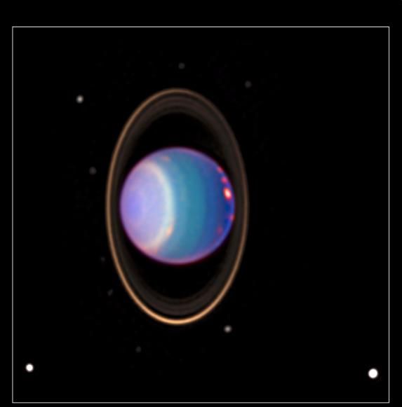
< 0.007 ISO SWS/LWS Burgdorf et al. (2003)3.2. Temperature 27 Figure 3.1: Equatorial temperature/pressure profiles of the giant planet atmospheres. Jupiter: solid line, Saturn: dotted line, Uranus: dashed line, Neptune: dot-dashed line. Reproduced from Irwin (2009), used by permission of author. cooling. The stratosphere is composed of stable, stratified layers. The boundary between these two layers is called the tropopause. On the giant planets, once the tropopause is passed and the stratosphere entered, temperature rises with height due to the high levels of CH4 absorbing solar radiation from the UV region through the IR. This research will focus on the observable regions of the upper troposphere and the strato- sphere. The relative minimum atmospheric temperature reached at the tropopause is about 50 K on Uranus, and occurs at approximately 100 mbar (Conrath et al., 1991b, 1998). The values for tropopause temperature and height are similar on Neptune (Bishop et al., 1995; Conrath et al., 1998). The ice giant tropopauses are thus some 50 – 100 K cooler than the corresponding regions of the gas giants, as shown in figure 3.1. The exact nature of the energy balance on the ice giants is poorly understood. Marley and McKay (1999) provide a thorough discussion of the leading theories, and maintain that the stratospheric temperatures of these bodies are regulated primarily by absorption of and emission by ethane (C2 H6 ) and acetylene (C2 H2 ). There is still much disagreement about the specific nature of the thermal mechanisms in the Uranian stratosphere (10−3 < p < 10−1 bar), in particular. Most attempts to model this region are unsuccessful at producing
3.3. Stratospheric Composition                                                          28

sufficiently high temperatures. Marley and McKay (1999) maintain that methane emission
plays the largest role heating this region, while most earlier studies seem to conclude, as
in Lindal et al. (1987), that the warmer layers discovered are a result of stratospheric
aerosol absorption of solar radiation.

3.3     Stratospheric Composition

Though many abundance profiles exist for trace constituents in Jupiter and Saturn’s
observable atmosphere, much less is known about trace gases on the icy giants. More
difficulty arises on Uranus and Neptune since the thermal radiation is much lower than
the gas giants, yielding very poor signal to noise ratios for infrared spectroscopy. In
addition, the larger distances involved, and the small number of satellite observations
have also limited the quality and quantity of results.

Despite these difficulties, some success has been achieved using IR data from the Voyager
2 flybys, as well as ISO, HST, Spitzer, and AKARI. In the last few years, as telescope
data has improved, publications have also begun to provide analysis of ground-based
IR observations. In addition to IR spectroscopy, many results have come from various
other remote sensing techniques including ground-based microwave, ground-based hy-
drogen quadrupole, and radio-occultation. Though the specific physics of these non-IR
techniques are beyond the scope of this report, the findings will be included in order to
paint a better picture of the composition of the ice giant atmospheres. This section out-
lines the most important information on stratospheric abundances, with complete results
to date summarised in tables 3.3 and 3.4.

With so many prominent absorption features and a relatively high abundance, strato-
spheric methane on the ice giants has been studied quite successfully. Stratospheric levels
are generally thought to be quite low, since the ice giant atmospheres are sufficiently cold
to trap most hydrocarbons below the tropopause (see section 3.5). Very small strato-
spheric CH4 abundances are found on Uranus, with no evidence for values above 10-5
(Orton et al., 1987a; Yelle et al., 1989; Encrenaz et al., 1998). Stratospheric CH4 abun-
dances are slightly higher on Neptune, with values on the order of 10−4 (Orton et al.,
3.3. Stratospheric Composition                                                        29

     Table 3.3: Stratospheric Composition of Uranus (updated   from Irwin, 2009)
  Gas     Mole Fraction               Measurement                Reference
                                      Technique
  H2 O    (6-14) ×10 at p < 0.03
                     −9
                                      ISO/SWS                   Feuchtgruber et al.
          mbar                                                  (1997)
  CH4     1×10⁻⁵                      Ground-based 12 �m        Orton et al. (1987a)
          (1-3) ×10 at p > 3 mbar Voyager far-UV
                    −7
                                                                Yelle et al. (1989)
          3×10⁻⁷ at 3 < p < 5 mbar
          (0.3-1) ×10−4 at            ISO/SWS                   Encrenaz et al. (1998)
          tropopause
          < 3 ×10⁻⁴ at 0.1 mbar
  CO      < 4.3 ×10⁻⁸                 Ground-based mm           Rosenqvist et al.
                                                                (1992)
          < 3.0 ×10⁻⁸                  Ground-based 1 mm        Marten et al. (1993)
          < 2.7 ×10⁻⁸                  Ground-based 1-3 mm      Cavalié et al. (2008)
  HCN     < 1.0 ×10⁻¹⁰ at              Ground-based 1 mm        Marten et al. (1993)
          0.003 < p < 30 mbar
  C2 H6   < 2×10⁻⁸                     Ground-based 12 �m       Orton et al. (1987a)
          < 3 ×10⁻⁶ at 0.1 mbar        Modelled                 Encrenaz et al. (1998)
          < 5 ×10⁻³ at p < 0.5         ISO/SWS                  Bézard et al. (2001)
          mbar
          ∼4 × 10⁻⁶                    Ground-based 12 �m       Hammel et al. (2006)
          (1.0 ± 0.1) × 10−8 at 0.1    Spitzer 10-20 �m         Burgdorf et al. (2006)
          mbar
  C2 H2   < 9×10⁻⁹                     Ground-based 12 �m       Orton et al. (1987a)
          10−8                         Voyager far-UV           Yelle et al. (1989)
          4×10⁻⁴ at 0.1 mbar           ISO/SWS                  Encrenaz et al. (1998)
          < 3.6 ×10⁻³ at p < 0.5       ISO/SWS                  Bézard et al. (2001)
          mbar
  C4 H2   (1.6 ± 0.2) × 10−10 at 0.1   Spitzer 10-20 �m         Burgdorf et al. (2006)
          mbar
 CH3 C2 H (2.5 ± 0.3) × 10−10 at 0.1   Spitzer 10-20 �m         Burgdorf et al. (2006)
          mbar
  CH3     not detected                 Spitzer 10-20 �m         Burgdorf et al. (2006)
          < 2.8 ×10⁻³ at p < 0.5       ISO/SWS                  Bézard et al. (2001)
          mbar
  CO2     (4 ± 0.5) × 10−11 at 0.1     Spitzer 10-20 �m         Burgdorf et al. (2006)
          mbar
          ≤ 3 × 10⁻¹⁰                  ISO/SWS                  Feuchtgruber et al.
                                                                (1997)
3.3. Stratospheric Composition 30
Table 3.4: Stratospheric Composition of Neptune (updated from Irwin, 2009)
Gas Mole Fraction Measurement Technique Reference
H2 O (1.5-3.5) ×10 −9
at p < 0.6 ISO Feuchtgruber et al. (1997)
mbar
CH4 < 0.02 Ground-based mid-IR Orton et al. (1987a)
7.5 +18.6
−5.6 × 10
−4
Ground-based mid-IR Orton et al. (1992)
3.5 × 10⁻⁴ Visible reflectance Baines and Hammel
(1994)
9 × 10⁻⁴ at 50 mbar AKARI/IRC Fletcher et al. (2010)
9 × 10⁻⁵ at 1 �bar
CO (6.5 ± 3.5) × 10−7 Ground-based 1-1.3 mm Rosenqvist et al. (1992)
(1.2 ± 0.36) × 10−6 Ground-based 1 mm Marten et al. (1993)
2.7 ×10⁻⁷ at 30-800 mbar HST UV reflectance Courtin et al. (1996)
< 1×10⁻⁶ (6 × 10⁻⁷ preferred) Ground-based 1-1.5 mm Encrenaz et al. (1996)
(1.0 ± 0.2) × 10−6 Ground-based 1 mm Marten et al. (2005)
0.5 ×10⁻⁶ at p > 20 mbar Ground-based 1 mm Marten et al. (2005)
1.0 ×10⁻⁶ at p < 20 mbar
(0.6 ± 0.4) × 10−6 (lower Ground-based 1mm Hesman et al. (2007)
stratosphere) increasing to
(2.2 ± 0.5) × 10−6 (upper
stratosphere)
HCN (3 ± 1.5) × 10−10 Ground-based 1-1.3 mm Rosenqvist et al. (1992)
(1.0 ± 0.3) × 10−9 at 0.003-30 Ground-based 1 mm Marten et al. (1993)
mbar
(3.2 ± 0.8) × 10−10 at 2 mbar; Ground-based 1.1 mm Lellouch et al. (1994)
approx. constant w/ height,
condenses at 3 mbar
1.5 × 10⁻⁹ at p < 0.3 mbar, Ground-based 1 mm Marten et al. (2005)
decreasing at lower altitudes
C2 H6 < 6 × 10⁻⁶ Ground-based 12 �m Orton et al. (1987a)
(2.5 ± 0.5) × 10−6 Voyager mid-IR Bézard and Romani
(1991)
(0.2-1.2) ×10−6 Ground-based mid-IR Orton et al. (1992)
< 5.4 × 10⁻⁴ at p < 1 mbar ISO/SWS Bézard et al. (2001)
(8.5 ± 2.1) × 10−7 at 0.3 mbar AKARI/IRC Fletcher et al. (2010)
C2 H2 < 9 × 10⁻⁷ Ground-based 12 �m Orton et al. (1987a)
6 +14
−4 × 10
−8
Voyager mid-IR Bézard and Romani
(1991)
(0.6-7.1) ×10−8 Ground-based mid-IR Orton et al. (1992)
(9-90)×10−8 Voyager IRIS Conrath et al. (1998)
< 5.4 × 10⁻⁴ at p < 1 mbar ISO/SWS Bézard et al. (2001)
C4 H2 (3 ± 1) × 10−12 at 0.1 mbar Spitzer 10-20 �m Meadows et al. (2008)
C2 H4 < 3 × 10⁻⁹
Ground-based 12 �m Orton et al. (1987a)
+1.8
5.0 −2.1 × 10⁻⁷ at 2.8 �bar AKARI/IRC Fletcher et al. (2010)
CH3 C2 H (1.2 ± 0.1) × 10−10 at 0.1 mbar Spitzer 10-20 �m Meadows et al. (2008)
CH3 ∼3.3 × 10 at p3.3. Stratospheric Composition 31 1992; Baines and Hammel, 1994; Fletcher et al., 2010). Fletcher et al. found their values consistent with the theory of a breakdown in the tropopausal cold trap at the south polar region that allows CH4 to ‘leak’ into the stratosphere. When small amounts of methane escape the troposphere, they often dissociate when photons bombard them in the thin, high-altitude air. This photolysis, and the resulting molecules and radicals (H2 , H, CH, CH2 , and CH3 ) serve to enrich the atmosphere with various hydrocarbons which form from products of the photolytic process. Acetylene (C2 H2 ) forms readily on both ice giants, and ethane (C2 H6 ) forms frequently on Neptune (Encrenaz, 2004). One stratospheric constituent that has sparked research in recent years is hydrogen cyanide (HCN). This is largely due to the unanswered question of where the molecule’s nitrogen might originate. Rosenqvist et al. (1992) detected HCN mole fractions in the Neptunian stratosphere of (3 ± 1.5) × 10−10 , suggesting that the molecule is produced by reactions between CH3 and N, the latter supplied by thermal escape from Triton’s atmosphere. Marten et al. (1993) detected higher levels of HCN on Neptune ((1 ± 0.3) × 10−9 between 0.003 and 30 mbar). They suggested that the particle’s presence could not be fully explained by the small amount of nitrogen escaping from Triton, but rather from upward transport of CO and N2 from Neptune’s deep interior. The same paper cited an upper limit for HCN in the Uranian stratosphere between 0.003 and 30 mbar of 1.0×10⁻¹⁰ . This upper limit was based on lack of internal heat to drive upward convection of required levles of CO and N2 (see section 3.4.3). Lellouch et al. (1994) detected a HCN abundance of (3.2 ± 0.8)×10−10 at 2 mbar on Neptune, stating the abundance should be approximately constant with height until the condensation level at 3 mbar. Marten et al. (2005),however, derived an abundance of 1.5 × 10⁻⁹ above 3 mbar, decreasing at lower altitudes. As described, no firm consensus has been reached about the Neptunian abundance profile of HCN, or the origin of the nitrogen required for HCN synthesis. Oxygen is another molecule that has been the subject of fervent study and speculation in the ice giants’ stratospheres. Stratospheric CO, CO2 , and H2 O have been detected on both Uranus and Neptune, and the existence of these molecules raises the question of where the oxygen, necessary for their production, comes from. Most H2 O in the ice giants
3.4. Dynamics                                                                               32

should be trapped below the cold tropopause, so most of the stratospheric H2 O must come
from external sources. CO2 can be formed by either using externally derived oxygen or
from stratospheric reactions between H2 O and CH3 . External sources for oxygen could
be small meteoroids, silicate dust particles, or simply an interplanetary flux of water ice
from the rings and satellites of the ice giants. It is estimated that approximately 105 -106
molecules·cm-2 ·s-1 of H2 O is imported from these sources to the gas giants’ atmospheres.
Most recent studies, however, favour a combination of both internal and external oxygen
sources. There seems to be no consensus reached in the literature to date, as examples can
be found of papers that conclude oxygen must be derived from every possible combination
of internal and external sources (Rosenqvist et al., 1992; Marten et al., 1993; Courtin et al.,
1996; Feuchtgruber et al., 1997; Encrenaz, 2004; Encrenaz et al., 2004; Hesman et al., 2007;
Fletcher et al., 2010).

3.4     Dynamics

The atmospheric dynamics of the ice giants are probably those least understood in our
solar system. The information that is known raises some fascinating questions.

3.4.1     Thermal Forcing

The dynamics of any planetary atmosphere are driven by a combination of solar and
internal heating. Analysis of the Voyager 2 data from the 1986 Uranus flyby revealed a
planet with a miniscule internal heat flux, representing no more than 6% of the planet’s
total heat flux (Marley and McKay, 1999). This fact, combined with Uranus’ 98° axial
tilt, makes it a unique case in atmospheric forcing among the planets of our solar system.
During the Voyager 2 flyby, Uranus was near its northern winter solstice, therefore the
planet’s extreme obliquity meant the southern hemisphere was receiving nearly all of the
planet’s solar heat flux. Given the nearly constant solar forcing across the planet during
the 10 or 15 years leading up to the flyby, the dynamics and atmospheric circulation
of Uranus seemed, at the time, to be rather uninteresting and static. The only major
You can also read