Rent/price ratio for English housing sub markets using matched sales and rental data - White Rose ...
←
→
Page content transcription
If your browser does not render page correctly, please read the page content below

Accepted: 3 April 2019

DOI: 10.1111/area.12555

REGULAR PAPER

Rent/price ratio for English housing sub‐markets using matched
sales and rental data

Stephen Clark1                      | Nik Lomax2

1
  Leeds Institute for Data Analytics and
                                                        The ratio between the rental and sales values of residential properties are a much
School of Geography, University of
Leeds, Leeds, UK                                        studied statistic in the field of real estate economics. When these values do not
2
  School of Geography and Leeds Institute               keep pace with each other, and in particular when the ratio is low, some commen-
for Data Analytics, University of Leeds,                tators take this as an indication that there may be a housing bubble building. The
Leeds, UK
                                                        ratios are also of interest to potential property investors. These ratios are com-
Correspondence                                          monly computed on aggregate statistics derived from the housing market and as
Stephen Clark
                                                        such rarely provide any indication of sub‐market bubbles, that can occur with par-
Email: tra6sdc@leeds.ac.uk
                                                        ticular property types or regions of the country. In this study use is made of a
Funding information                                     data set from a property listings company that provides sales and, potentially, ren-
ESRC Consumer Data Research Centre,
                                                        tal prices for the same properties within England. From the matching that takes
Grant/Award Number: ES/L011891/1
                                                        place it is possible to calculate the rent/price ratio for individual properties. A
                                                        regression model is then estimated to explain how the characteristics of the prop-
                                                        erties; the nature of their neighbourhood; and their location influence this ratio.
                                                        The model consistently validates the hypothesis that the more desirable a property
                                                        or affluent an area, the lower the rent/price ratio. It also begins to illustrate the
                                                        range of “normal” rent/price ratios that may exist in housing sub‐markets. The
                                                        regression model is then used to provide a map of the geographical distribution of
                                                        the ratio for England for one property sub‐market.

                                                        KEYWORDS
                                                        house rental, house sales, regression, rent/price ratio, sub-markets

1     | INTRODUCTION
Housing is one of the largest items of household expenditure for families; in the United Kingdom (UK) it is the third lar-
gest outgoing, after transport and recreation (Office for National Statistics, 2018). The 2011 Census reports that in England,
31% of households owned their property outright, 33% had a mortgage, 18% were socially rented, 17% were privately
rented, and 2% were either shared ownership or rent free. Trends since 2011 however point to a reduction in the proportion
of residential properties that are owned, mortgaged, or socially rented, and an increase in those that are privately rented
(Lund, 2013). The latest to 2015 show that the proportion of households that are privately rented has risen to 20% (Valua-
tion Office Agency, 2015; Wilcox et al., 2017).
    These trends are driven by: changes to policy around the support given to renters (Stephens & Whitehead, 2014); the
availability of de‐socialised housing stock (Copley, 2014); and the attractiveness of rental properties for landlords (Ronald

----------------------------------------------------------------------------------------------------------------------------------------------------------------------
This is an open access article under the terms of the Creative Commons Attribution License, which permits use, distribution and reproduction in any medium, provided the
original work is properly cited.
The information, practices and views in this article are those of the author(s) and do not necessarily reflect the opinion of the Royal Geographical Society (with IBG).
© 2019 The Authors. Area published by John Wiley & Sons Ltd on behalf of Royal Geographical Society (with the Institute of British Geographers).

136   |   wileyonlinelibrary.com/journal/area                                                                                                        Area. 2020;52:136–147.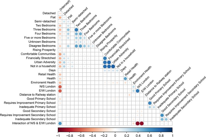
CLARK   AND   LOMAX                                                                                                           |   137

& Kadi, 2018), particularly as investments (Mellish & Rhoden, 2009; Sprigings, 2008). One particular demographic often
cited as challenged by these changes in the housing market is “generation‐rent,” young people who are unable to afford to
buy a home, are denied access to the limited social rented sector (Schmickler & Park, 2014), and are therefore reliant on
private rented properties (Alakeson, 2011; Clapham et al., 2014; Lund, 2013). In such a diverse and dynamic market it is
important to have an understanding of the mechanisms at work that affect price and affordability and how these differ by
sub‐markets, either in terms of the type of property or by geography.
    One important measure of the state of the housing market is the rent/price ratio yield, which is calculated as the annual
rental value of a property divided by its sale price. However, there are a number of nuances to this definition (Wyatt,
2013). The first aspect is whether the rental yield is based on gross or net costs. In regards to the rent, the net rent could
reflect the rental costs, e.g., agent management fees or property maintenance, and in regards to sales, the net sales price
could reflect the on‐costs of the purchase, e.g., legal or mortgage loan fees. A second aspect concerns whether the rent is
the current rent charged (initial yield) or the market rent (reversionary yield), where over time, unless the rent is re‐nego-
tiated, the two will diverge. Notwithstanding these nuances, typically the rent/price ratio has a value around 0.06.
    The utility of this ratio rests with both its ability to identify possible housing bubbles (Mayer, 2011; Smith & Smith,
2006) and also to indicate potential investment yields from buy‐to‐let purchases (Leyshon & French, 2009). Ideally the ratio
should be calculated on the same stock of housing, but practical difficulties usually make this problematic – houses rarely
appear on the market at the same time for rent and sale, and when they are either rented or sold the alternative value mea-
sure is unrealised. Recognising this, the ratio is commonly calculated based on an aggregate understanding of the trends in
rents and house prices. In this paper the rent/price ratio will be calculated using a method that matches contemporaneous
sales and rental data for the same property within England by making use of administrative and commercial property data
sources. This technique will allow an almost complete picture and understanding of the pattern of this ratio by aspects of
the property, its neighbourhood, and its geography. No previous studies have attempted this task on this scale – the closest
are a study confined to the atypical West London housing market (Bracke, 2015) and the calculation of correction factors
to apply to modelled rents and prices in Sydney, Australia (Hill & Syed, 2011).
    Section 2 of this paper provides some background on the rent/price ratio and how it has been used in previous studies.
Section 3 introduces the data and the methodology used to calculate the ratio. Section 4 presents the results of a regression
model that attempts to show how various attributes influence the ratio, and maps national estimates of the ratio for English
postcodes. Finally, section 5 provides a discussion of these findings and the wider implications of the work.

2   | IMPORTANCE OF THE RENT/PRICE RATIO
The importance of the rent/price ratio to politicians, policy analysts, and economists is that it reflects the stability of a hous-
ing market or its sub‐markets. In a stable housing market the ratio will remain relatively consistent. However, if the ratio
begins to fall then there is evidence that the value of the underlying asset, the property, is beginning to increase (Campbell
et al., 2009). When this departure occurs, there is usually a correction, which can be through a gradual convergence as rents
also increase, or a sudden drop in the property price – a burst bubble (Ambrose et al., 2013; Jurgilas & Lansing, 2012).
Various econometric models have been estimated to try to gain an understanding of how useful the rent/price ratio is in
predicting a bubble. This has been done for the UK (Kim, 2015; Ngai & Tenreyro, 2014); the Euro area (Hiebert & Sydow,
2011); a range of OECD counties (André et al., 2014; Engsted & Pedersen, 2015); China (Zhai et al., 2017); the USA
(Gallin, 2008; Kivedal, 2013); and a selection of Metropolitan areas within the USA (Beracha et al., 2012; Campbell et al.,
2009; Kishor & Morley, 2015). Many of these studies report that the ratio is a valid indicator for the development of a
property bubble. In particular, studies of the Metropolitan Areas of the USA identified markets that were subject to a bub-
ble that burst and those that also experienced some form of bubble but in which the correction was less severe. This varia-
tion in outcome is also evident in European countries: Spain and Ireland experienced a bubble followed by a burst, but
Germany did not (Hiebert & Sydow, 2011). The question then arises as to what is driving these departures from the funda-
mental relationship between rents and property prices? Some of these drivers include: interest rates, levels of housing
affordability, regulatory environment, taxation and tax relief, speculation, constraints on development, and demographics
(Clark & Coggin, 2011; Mayer, 2011).
    Another important use of the rent/price ratio is to establish a likely rental yield from owning and renting out a property.
Kennett et al. (2013) and Whitehead and Williams (2011) chart UK trends in the private rental market from a period of
slow decline until the 1990s, followed by a period of stability and then rapid growth, starting in the early years of the 21st
century. The impact of the global financial crisis in 2007/2008 is seen to encourage the private rental market due to a
138
| CLARK AND LOMAX
“search for yield” in a global environment of low interest rates, which provides poor yields from monetary deposits and
also makes borrowing to invest in property more attractive. However, it is argued that it is more the potential for capital
gain than rental income that is of interest to investors (Kemp, 2015).
3 | DATA AND METHODOLOGY
The rental and sales data for this study is primarily collected by Zoopla (2018), a large online property listing company
which has been processed by the data services company WhenFresh, with additionally the sales data being supplement with
administrative data from the Land Registry (Her Majesties’ Land Registry, 2018). The data cover the calendar years 2014
and 2015.
For all sales, the property type (flat, terrace, semi‐detached, and detached), its address, the date of the sale transaction,
and the sale price are available. When this sale was also listed on the Zoopla web site, additional data concerning the prop-
erty is available, including the number of bedrooms. For rental properties only information from Zoopla is available, which
included: property type, date of listing, rental price listed, and number of bedrooms.
Prior to its use some cleaning of these data takes place. Transactions before January 2014 and after December 2015 are
removed, exact and temporally close (within seven days) duplicates are deleted and outliers are removed. The removal of
outliers in these types of commercial data is commonplace (Ambrose et al., 2015; Bracke, 2015; McCord et al., 2014) and
here, rather than the top and bottom slicing of a fixed percentage of the distribution of asking rents or actual sale prices, a
variation of the approach to identifying outliers in a box‐plot is used. First the listings are segmented into sub‐markets by
property type, number of bedrooms, and the Acorn Category of the postcode for the property (CACI, 2017) (these cate-
gories will be introduced below). A lower limit for the rent or price is then set as 1.5 times the inter‐quartile range below
the lower quartile and the upper limit as 3.0 times the inter‐quartile range above the upper quartile. The asymmetry in the
multipliers is a recognition that these data are not symmetric, exhibiting a positive skew. Thus the identification of outliers
is only made in the context of similar properties and no fixed percentage of outliers are forced to be removed. In practice
this approach removes just 1.8% of rental listings and 1.3% of sales listings. In total, all these cleaning operations remove
just over 10% of rental listings and only 2% of sales.
The methodology here adopts that of Bracke (2015), where the same property is identified in the sales data and the ren-
tal data and those properties where the rental occurs between one and eight months after the sale are retained. The same
properties are identified using the full address and the postcode. For the sales data, no information on the size of property,
e.g., number of bedrooms, is available where the data are sourced from the Land Registry and is also sometimes missing
from the Zoopla listing. Other studies have attempted similar exercises – including exact matching for sales and rentals
(Bracke, 2015); exact repeat rentals (Ambrose et al., 2015); identifying similar sales and rental properties (Smith & Smith,
2006); and developing hedonic rental and sales price models to estimate, for the same property, a contemporary sales and
rental value (Hill & Syed, 2011).
After the merging of the two datasets a comparison of the property aspects can be made, one piece of information from
the sales data and one from the rental listing. Here there are some discrepancies. Table 1 gives the cross‐tabulation of prop-
erty type. The comparison is complicated by the absence of the bungalow category in the Land Registry sales data: bunga-
lows can be detached or semi‐detached (but not flats or terraced!). Also, sometimes an end terrace house may be listed as
semi‐detached. The illogical cross‐classifications are shown as italics and shaded in dark grey in Table 1 and amount to just
less than 5% of properties. Taking this information forward, the property type is taken from the more complete Land
T A B L E 1 Cross‐tabulation of property type from sales and rental data
Rental
Sales Not known Bungalow Detached Flat Semi‐detached Terrace
Detached 222 275 658 35 53 20
Flat 327 6 26 8,608 13 71
Semi‐detached 825 275 90 131 2,541 282
Terraced 2,495 56 253 446 734 7,061
Note: Bold values are consistent from the two sources; light grey values are known from one source only; italic values in dark grey signify values that are inconsis-
tent; and normal cells are values that could be consistent. These counts sum to 25,503, however 600 of these properties do not have a valid postcode and therefore
are not used in the summary statistics reported in Table 3 or the regression results reported in Table 4.CLARK AND LOMAX | 139
T A B L E 2 Cross‐tabulation of number of bedrooms from sales and rental data
Rental
Sales 1 Bedroom 2 Bedrooms 3 Bedrooms 4 Bedrooms 5 or more Bedrooms Not known
1 Bedroom 1,884 111 20 1 0 58
2 Bedrooms 123 5,832 387 46 12 77
3 Bedrooms 241 153 4,883 408 105 84
4 Bedrooms 91 17 71 691 106 29
5 or more Bedrooms 48 16 11 25 235 14
Not known 1,967 3,802 2,709 610 247 389
Note: Bold values are consistent from the two sources; light‐grey values are known from one source only; and italic values in dark grey signify values that are
inconsistent. These counts sum to 25,503, however 600 of these properties do not have a valid postcode and therefore are not used in the summary statistics reported
in Table 3 or the regression results reported in Table 4.
Registry data. The situation is more complex for the number of bedrooms, as shown in Table 2. There is straightforward
agreement along the main diagonal for 53% of properties plus a further 1.5% where neither source provides any information
(bold and white cells). For 38% of properties, only one source has information (normal and light grey cells), leaving just
8% where there is active disagreement between the two sources (italic and dark grey). This disagreement could be due to
renovation work carried out between the dates of the sale and the rental listing to either remove or add a bedroom to the
property, but this reason is unlikely to explain all of these discrepancies. Taking this forward, where there is agreement, this
information is used; where only one piece of information is known, this is used; and where they disagree, this is marked as
a property with an active disagreement.
Information on the number of days between the sale and the rental listing is recorded. Additionally, based on the prop-
erty's postcode, the following information is attached to the property: its Acorn geodemographic profile; its score on three
health indices (Daras et al., 2018); its distance north/south and east/west of Kensington Palace in West London; distance
from the nearest railway/underground station (Department for Transport, 2017); and the Ofsted rating of the nearest primary
and secondary schools (Baxter & Clarke, 2013).
From the 101,324 properties that match between sales and rental listing, those where the subsequent rental occurs
between one and eight months after the sale are identified. When all this information is collected together, the summary
statistics for the sales data, the rental data and the matched data are provided in Table 3. The rent/price ratio yield is calcu-
lated as the annual asking rent of the property divided by the sales price. Such a yield is best described as a reversionary
gross yield, since the costs are those that reflect current market conditions and also do not reflect any of the costs associ-
ated with the transaction. Of those rental properties listed on the Zoopla rental site, 2.5% were sold within the previous one
to eight months. The matched data have higher rents but lower sales prices, and thereby a higher rent/price ratio. There is
more terraced housing in the matched data set and the properties are smaller, with a predominance of two bedrooms. Fewer
of the matched properties are located in areas with the affluent achievers geodemographic classification and more are to be
found in the Financially Stretched and Urban Adversity areas. Matched properties are located closer to London. The distri-
butions of primary and secondary school Ofsted ratings are similar among all three data sets.
4 | REGRESSION RESULTS
Using the matched data set, a regression equation is used to try and understand the predictors of the rent/price ratio and pro-
vide a model to predict the rent/price ratio for each English postcode (see Table 4). Since the ratio is positively skewed and
the mean and variance are not similar, a quasi‐Poisson generalised linear model is fitted using the glm function in R (R Core
Team, 2016) with a quasi‐Poisson family (Fox, 2015). Detached or semi‐detached houses have a lower ratio than terraced
houses, while flats have a higher ratio. The more bedrooms that a property has, the higher the ratio. The longer the gap
between the property being sold and listed on the rental market, the higher the ratio. As the affluence of the area decreases,
then the ratio increases. Living in an area with a healthy retail location and good access to health services decreases the rent/
price ratio, while a healthy physical environment increases the ratio. The further from central London, in any direction, the
higher the ratio. A greater distance to the nearest railway or underground station has a negative impact on the ratio but is not
significant. In terms of primary schools, the ratio increases relative to the base of having an school rated as Outstanding by
Ofsted close by, but only significantly so for Good and Requires Improvement schools. For secondary schools, the ratio140
| CLARK AND LOMAX
T A B L E 3 Comparative statistics between the three data sets (proportion unless otherwise stated)
Attribute Variablea Matched Sales Rental
Observations (n) NA 1,828,646 1,204,913
After filtering (n) NA 24,903 1,796,814 1,083,918
Median annual rent (£) NA £9,308 £8,996
Median sales price (£) NA £160,000 £199,000
Rent/price (ratio) Real 0.0582 0.0452 0.0452
Terraced Base 0.43 0.29 0.23
Flat 0/1 0.36 0.20 0.43
Semi‐detached 0/1 0.16 0.26 0.11
Detached 0/1 0.05 0.25 0.07
Bungalow 0/1 0.03
Unknown 0/1 0.14
One bedroom Base 0.17 0.03 0.19
Two bedrooms 0/1 0.41 0.15 0.39
Three bedrooms 0/1 0.32 0.23 0.26
Four bedrooms 0/1 0.06 0.09 0.09
Five or more bedrooms 0/1 0.02 0.02 0.04
Unknown 0/1 0.02 0.48 0.03
Disagree 0/1 0.08
Affluent Achievers Base 0.09 0.23 0.12
Rising Prosperity 0/1 0.22 0.14 0.27
Comfortable Communities 0/1 0.23 0.30 0.20
Financially Stretched 0/1 0.21 0.15 0.18
Urban Adversity 0/1 0.24 0.10 0.18
Not in private households 0/1 0.00 0.01 0.01
Unknown 0/1 0.00 0.08 0.04
Retail health (score) Real 30.45 16.71 29.94
Health services (score) Real 7.17 15.46 7.47
Environmental health (score) Real 24.46 18.79 24.68
Distance N/S of London (km) Real 67.92 84.78 74.05
Distance E/W of London (km) Real 66.20 80.30 69.30
Distance to nearest railway/underground (km) Real 1.08 1.67 1.14
Primary school
Outstanding Base 0.17 0.17 0.19
Good 0/1 0.63 0.63 0.63
Requires improvement 0/1 0.17 0.18 0.16
Inadequate 0/1 0.02 0.02 0.02
Secondary school
Outstanding Base 0.23 0.20 0.24
Good 0/1 0.50 0.51 0.51
Requires improvement 0/1 0.21 0.23 0.20
Inadequate 0/1 0.06 0.06 0.05
a
Note: Real is a continuous measure; Base the base category for a categorical variable; 0/1 is a conversion from a categorical variable into a series of binary vari-
ables; NA is a variable not explicitly used in the model.CLARK AND LOMAX | 141 T A B L E 4 Regression of rent/price index Attribute Estimate Standard error t‐Value Significance Impact (%) Constant −3.3996 0.0212 −160.50
142
      |                                                                                                         CLARK   AND   LOMAX

T A B L E 5 Summary fit statistics
 Statistic                                                                 Log scale                              Original scale
 Root mean square error                                                    0.3251                                  0.0236
 Mean absolute error                                                       0.2207                                  0.0146
 Mean absolute percentage error                                            8.11                                   26.10
 Median absolute percentage error                                          5.71                                   15.85

F I G U R E 1 Parameter estimates correlation matrix. [Colour figure can be viewed at wileyonlinelibrary.com]

intercept, the highest correlation is 0.721, which is between the north/south and the east/west of London. Using the vif
function in R package car (Fox & Weisberg, 2011), the highest GVIF1/(s*dof) value is 4.87 for the distance from London
interaction term, which does not indicate a severe problem with multi‐collinearity (see O'Brien (2007) for a discussion on
suitable rules of thumb).
    Using the glm model it is then possible to estimate the rent/price ratio for areas in England for a given property type.
Looking at the terms in the regression, all are known at the geography of postcode, except the number of days between the
sale and rental. To provide this information the median number of days between the sale and rental listing by property type
and number of bedrooms is used (Table 5 provides a count of this distribution and Table 6 the median time gap, which for
the majority of properties is just less than three months). The map of these ratios for a two‐bedroom flat (the most com-
monly matched property type) is provided in Figure 2, with the ratio split into quintiles. The ratio is highest in a band
across northern England, from Liverpool in the west, eastwards through Manchester and West Yorkshire and then running
south through the East Midlands. It also appears to be lower in rural postcodes relative to the nearest major town or city,
with rural properties commanding high sales prices, since they are often purchased as premium, retirement, or second prop-
erties, but being unable to command high rents, since local employment opportunities can be limited in rural postcodes.
Also the distance from London impact is seen to be mitigated somewhat, with some rural postcodes in the north having a
ratio not dissimilar to that in the Home Counties around London.
CLARK AND LOMAX | 143
T A B L E 6 Number of 1–8‐month matched properties, by property type and number of bedrooms
1 Bedroom 2 Bedrooms 3 Bedrooms 4 Bedrooms 5 or more bedrooms Unknown Disagree
Terraced 628 3,894 4,016 687 245 60 1,144
Detached 23 186 502 289 105 3 109
Flat 3,106 4,562 604 74 11 299 320
Semi‐detached 112 882 2,297 246 102 23 374
F I G U R E 2 Estimated rent/price ratio for two‐bedroomed flats for a sample of English postcodes. [Colour figure can be viewed at
wileyonlinelibrary.com]
5 | DISCUSSION
In this paper we determine the rent/price ratio for a heterogeneous mix of properties types for every postcode in England.
The information is derived from a mix of commercial (rental/sales) and administrative (sales) data sources. The work has
been extended to a model that explains these ratios using a combination of information about the property, the affluence of
the area, and the neighbourhood characteristics.144
| CLARK AND LOMAX
A consideration of the results reported in Table 4 reveals some insight into the rent/price ratio. Relative to terraced
houses, flats have a higher ratio, while detached and semi‐detached properties have a lower ratio, a reflection of their sales
price differentials relative to terraced properties. This finding shows that, all other things being equal, flats have the highest
ratio, followed by terraced properties. The greater the number of bedrooms, the higher the ratio, with the premium for two
bedrooms over one being just over 2%, but for five or more bedrooms it is much greater at more than 20%. This indicates
that while larger properties sell for higher prices, their rarity on the rental market allows a premium to be incorporated in
the expected rent and such a higher rent will increase the ratio. Where the number of bedrooms is either unknown or there
is some disagreement, the estimate is somewhere between that for two and three bedrooms. A longer time between the sale
and rental listing may reflect the fact that some renovation work is required to the property, which means that it was proba-
bly sold for a lower sales price, but this work would also lead to a higher expectation for the rent, and hence, as seen here,
a higher ratio. Although the reported percentage impact per day is low, over a gap of 100 days (not untypical, see Table 7),
this multiplies out to a 3% increase in the ratio. A general finding in other studies is that wealth or affluence tends to pro-
duce a lower rent/price ratio (Bracke, 2015) and this is reflected in the results reported for the Acorn geodemographic cate-
gories, as affluence decreases, the ratio increases. This is where the highest impact values are seen, with a near 50%
increase in the ratio for challenged areas of Urban Adversity. Living in a neighbourhood with a healthy retail environment
(away from fast food restaurants, tobacconists and gambling) and access to health services reduces the ratio but conversely
a neighbourhood with good physical environmental health (in terms of lower pollution levels and access to green space)
increases the ratio. These scores are measured on a scale of 0–100, so the scope for large changes and hence large percent-
age impacts on the ratio are limited. The variable that explicitly captures the spatial aspects of the ratio is the distance from
West London, differentiated by both a north/south axis and an east/west axis plus an interaction term. The further from
London (in log terms), the higher the ratio, which is a reflection of high property prices in West London that may struggle
to be matched with similarly high rents. A 10% increase in distance from London north or south is much more pronounced
(over three times more) than a similar increase east or west of London. For primary and secondary schools, the neighbour-
hoods in the catchment of schools that are not Outstanding have higher ratios, another reflection of the ratio being higher
in less affluent neighbourhoods, with properties in such neighbourhood been relatively cheap to buy but still able to com-
mand a reasonable rent. The impact of the secondary school's rating is much higher than that of the primary school.
Many of these findings, using a diverse range of attributes, confirm the hypothesis that deprivation tends to increase the
rent/price ratio. These interpretations also show that aspects that increase the sales price of a property (e.g., close to ameni-
ties and good schools) do not necessarily increase the rental value of a property, thereby enabling a significant variation in
the ratio to be attributed to these aspects.
This study is also revealing in terms of the utility of the rent/price to indicate a potential housing bubble. We have iden-
tified that there exists considerable variation in this ratio and attributed it to a diverse range of influences. A low ratio indi-
cates that properties are expensive relative to their potential rental yield. A low value of around 0.04 is not uncommon in
central London, but if observed elsewhere say, where the typical value is around 0.05 or 0.06, then that would indicate that
the property market, in that location, may be experiencing a bubble. This allows for regional bubbles in the housing market
to be identified.
From an investor perspective, this model suggests that the type of property with the highest rent/price ratio is a reno-
vated flat with a large number of bedrooms, in a less affluent area, at some distance from London. An investor with £10
million to invest and looking to maximise their gross rental yield would, rather than investing in a couple of properties in
West London, be better off investing in hundreds of properties in the less affluent areas of the Midlands and North. The
map in Figure 2 corroborates this, with the highest ratios and hence potential yields in areas of the Midlands and northern
England. Also capital appreciation is not guaranteed to offset this lower yield for London properties, with Land Registry
data showing London to be the only region of England to show a decline (from 119 to 117 points) in its house price index
in the 10‐month period to February 2018 (Land Registry, 2018).
T A B L E 7 Number of days between sales and rental listing, by property type and number of bedrooms
1 Bedroom 2 Bedrooms 3 Bedrooms 4 Bedrooms 5 or more bedrooms Unknown Disagree
Terraced 94 85 82 94 109 104 105
Detached 111 90 85 95 94 65 98
Flat 90 85 86 85 140 103 99
Semi‐detached 99 85 88 81 91 164 114CLARK AND LOMAX | 145
The equivalent Bracke (2015) study is more geographically limited than the work reported here. They only used data
for West London, which was primarily composed of high‐value flats, making the results difficult to generalise to the whole
of the UK. What Bracke (2015) was able to do was incorporate information on time between repeat rentals, rent apprecia-
tion, and rent volatility into the model, taking advantage of having a longer time series from 2006 to 2012. These later
terms improved the model fit considerably. In the data used for this study, the opportunities for repeat rents is limited: only
429 properties are listed for rent on two or more occasions after their sale. However, these repeat terms, which are very
property‐specific, would make any model difficult to generalise to the postcode geography.
The work reported here could be extended by incorporating either more historic information from before 2014 or, more
readily, data after 2015. Since the processing of these data is largely automated (in regards to the use of other data sources
and the modest cleaning of the data), this extension would be trivial in a data sense. However, it is the data acquisition that
is a challenge, with legal and procedure negotiations with data providers being necessary – particularly for the rental data,
which is not readily available from other sources. If a longer time span of data is available, it would then be possible to
split the data into time segments and use that analysis to gain an understanding of the short‐term trends in the rent/price
ratio, which would be of value to policy analysts and econometricians. Another extension is to repeat the analysis for other
housing markets, both in the UK and Europe, or anywhere that has access to the volume and variety of data used here
(e.g., Zillow in the USA (Zillow, 2018); RealEstate.com in Australia (Realestate.com.au, 2018); and Funda in the Nether-
lands (Funda, 2018)).
ACKNOWLEDGEMENTS
Contains HM Land Registry data © Crown copyright and database right 2018. These data are licensed under the Open
Government Licence v3.0. The authors acknowledge Zoopla as the data collector and WhenFresh the data provider. The
work was funded by the ESRC Consumer Data Research Centre, Grant No. ES/L011891/1. The authors would also like to
thank the reviewer of this article for their challenging and constructive comments.
DATA ACCESSIBILITY
Due to confidentiality agreements with research collaborators, supporting data can only be made available to researchers
subject to a non‐disclosure agreement. Details of the data and how to request access are available from the corresponding
author.
ORCID
Stephen Clark https://orcid.org/0000-0003-4090-6002
Nik Lomax https://orcid.org/0000-0001-9504-7570
REFERENCES
Alakeson, V. (2011). Making a rented house a home: Housing solutions for ‘generation rent’. London, UK: Resolution Foundation. Retrieved
from http://www.emcouncils.gov.uk/write/documents/resolution%20foundation%20housing_report_final.pdf
Ambrose, B. W., Coulson, N. E., & Yoshida, J. (2015). The repeat rent index. Review of Economics and Statistics, 97, 939–950. https://doi.org/
10.1162/REST_a_00500
Ambrose, B. W., Eichholtz, P., & Lindenthal, T. (2013). House prices and fundamentals: 355 years of evidence. Journal of Money, Credit and
Banking, 45, 477–491. https://doi.org/10.1111/jmcb.12011
André, C., Gil-Alana, L. A., & Gupta, R. (2014). Testing for persistence in housing price‐to‐income and price‐to‐rent ratios in 16 OECD coun-
tries. Applied Economics, 46, 2127–2138. https://doi.org/10.1080/00036846.2014.896988
Baxter, J., & Clarke, J. (2013). Farewell to the tick box inspector? Ofsted and the changing regime of school inspection in England. Oxford
Review of Education, 39, 702–718. https://doi.org/10.1080/03054985.2013.846852
Beracha, E., Seiler, M., & Johnson, K. (2012). The rent versus buy decision: Investigating the needed property appreciation rates to be indifferent
between renting and buying property. Journal of Real Estate Practice and Education, 15, 71–87.
Bracke, P. (2015). House prices and rents: Microevidence from a matched data set in central London. Real Estate Economics, 43, 403–431.
https://doi.org/10.1111/1540-6229.12062
CACI. (2017). What is ACORN? Retrieved from http://acorn.caci.co.uk/
Campbell, S. D., Davis, M. A., Gallin, J., & Martin, R. F. (2009). What moves housing markets: A variance decomposition of the rent‐price ratio.
Journal of Urban Economics, 66, 90–102. https://doi.org/10.1016/j.jue.2009.06.002146
| CLARK AND LOMAX
Clapham, D., Mackie, P., Orford, S., Thomas, I., & Buckley, K. (2014). The housing pathways of young people in the UK. Environment and
Planning A, 46, 2016–2031. https://doi.org/10.1068/a46273
Clark, S. P., & Coggin, T. D. (2011). Was there a US house price bubble? An econometric analysis using national and regional panel data. The
Quarterly Review of Economics and Finance, 51, 189–200. https://doi.org/10.1016/j.qref.2010.12.001
Copley, T. (2014). From right to buy to buy to let. Greater London Authority/London Assembly Labour.
Daras, K., Davies, A., Green, M., & Singleton, A. (2018). Developing indicators for measuring health-related features of neighbourhoods. In P.
Longley, J. Cheshire & A. Singleton (Eds.), Consumer data research. London, UK: UCL PRESS.
Department for Transport. (2017). National Public Transport Access Nodes (NaPTAN). Retrieved from https://data.gov.uk/dataset/naptan
Duan, N. (1983). Smearing Estimate – a nonparametric retransformation method. Journal of the American Statistical Association, 78, 605–610.
https://doi.org/10.2307/2288126
Engsted, T., & Pedersen, T. Q. (2015). Predicting returns and rent growth in the housing market using the rent‐price ratio: Evidence from the
OECD countries. Journal of International Money and Finance, 53, 257–275. https://doi.org/10.1016/j.jimonfin.2015.02.001
Fox, J. (2015). Applied regression analysis and generalized linear models. Los Angeles, CA: Sage Publications.
Fox, J., & Weisberg, S. (2011). An R companion to applied regression. Thousand Oaks, CA: Sage.
Funda (2018). Watching the sun rays fall into the living room. Retrieved from https://www.funda.nl/en/huur/
Gallin, J. (2008). The long‐run relationship between house prices and rents. Real Estate Economics, 36, 635–658. https://doi.org/10.1111/j.1540-
6229.2008.00225.x
Her Majesties’ Land Registry. (2018). Price paid data. Retrieved from https://www.gov.uk/government/collections/price-paid-data
Hiebert, P., & Sydow, M. (2011). What drives returns to euro area housing? Evidence from a dynamic dividend–discount model. Journal of
Urban Economics, 70, 88–98. https://doi.org/10.1016/j.jue.2011.03.001
Hill, R. J., & Syed, I. (2011). Hedonic price-rent ratios for housing: Implications for the detection of Departures from Equilibrium. UNSW Aus-
tralian School of Business Research Paper (2012).
Jurgilas, M., & Lansing, K. J. (2012). Housing bubbles and homeownership returns. FRBSF Economic Letter, 2012–19.
Kemp, P. A. (2015). Private renting after the global financial crisis. Housing Studies, 30, 601–620. https://doi.org/10.1080/02673037.2015.
1027671
Kennett, P., Forrest, R., & Marsh, A. (2013). The global economic crisis and the reshaping of housing opportunities. Housing, Theory and Soci-
ety, 30, 10–28. https://doi.org/10.1080/14036096.2012.683292
Kim, J. R. (2015). What drives the price‐rent ratio in the UK housing market? An Unobserved component approach. Journal of Marketing and
Management, 6, 74.
Kishor, N. K., & Morley, J. (2015). What factors drive the price–rent ratio for the housing market? A modified present‐value analysis. Journal of
Economic Dynamics and Control, 58, 235–249. https://doi.org/10.1016/j.jedc.2015.06.006
Kivedal, B. K. (2013). Testing for rational bubbles in the US housing market. Journal of Macroeconomics, 38, 369–381. https://doi.org/10.1016/
j.jmacro.2013.08.021
Land Registry. (2018). UK House Price Index. Retrieved from http://landregistry.data.gov.uk/app/ukhpi/
Leyshon, A., & French, S. (2009). ‘We all live in a Robbie Fowler house’: The geographies of the buy to let market in the UK. The British Jour-
nal of Politics and International Relations, 11, 438–460. https://doi.org/10.1111/j.1467-856X.2009.00381.x
Lund, B. (2013). A ‘property‐owning democracy'or ‘generation rent’? The Political Quarterly, 84, 53–60. https://doi.org/10.1111/j.1467-923X.
2013.02426.x
Mayer, C. (2011). Housing bubbles: A survey. Annual Review of Economics, 3, 559–577. https://doi.org/10.1146/annurev.economics.012809.
103822
McCord, M., Davis, P., Haran, M., McIlhatton, D., & McCord, J. (2014). Understanding rental prices in the UK: A comparative application of
spatial modelling approaches. International Journal of Housing Markets and Analysis, 7, 98–128. https://doi.org/10.1108/IJHMA-09-2012-
0043
Mellish, P., & Rhoden, M. (2009). “Buy to let”: A popular investment? Property Management, 27, 178–190. https://doi.org/10.1108/
02637470910964660
Ngai, L. R., & Tenreyro, S. (2014). Hot and cold seasons in the housing market. American Economic Review, 104, 3991–4026. https://doi.org/
10.1257/aer.104.12.3991
O'Brien, R. M. (2007). A caution regarding rules of thumb for variance inflation factors. Quality and Quantity, 41, 673–690. https://doi.org/10.
1007/s11135-006-9018-6
Office for National Statistics. (2018). Family spending in the UK: Financial year ending 2017. Retrieved from https://www.ons.gov.uk/peoplepop
ulationandcommunity/personalandhouseholdfinances/expenditure/bulletins/familyspendingintheuk/financialyearending2017
R Core Team. (2016). R: A language and environment for statistical computing. Vienna, Austria: R Foundation for Statistical Computing.
Retrieved from https://www.R-project.org/
Realestate.com.au (2018). Rental properties, homes and aparments for rent. Retrieved from https://www.realestate.com.au/rent
Ronald, R., & Kadi, J. (2018). The revival of private landlords in Britain's post‐homeownership society. New Political Economy, 23, 786–803.
https://doi.org/10.1080/13563467.2017.1401055
Schmickler, A., & Park, K. S. (2014). UK social housing and housing market in England: A statistical review and trends. LHI Journal, 5, 193.
Smith, M. H., & Smith, G. (2006). Bubble, bubble, where's the housing bubble? Brookings Papers on Economic Activity, 2006, 1–67. https://doi.
org/10.1353/eca.2006.0019CLARK AND LOMAX | 147
Sprigings, N. (2008). Buy‐to‐let and the wider housing market. People, Place and Policy Online, 2, 76–87. https://doi.org/10.3351/ppp.0002.
0002.0003
Stephens, M., & Whitehead, C. (2014). Rental housing policy in England: Post crisis adjustment or long term trend? Journal of Housing and the
Built Environment, 29, 201–220. https://doi.org/10.1007/s10901-013-9386-x
Valuation Office Agency. (2015). Private rental market summary statistics England, 2014–15. Retrieved from https://www.gov.uk/government/
statistics/private-rental-market-statistics-may-2015
Whitehead, C., & Williams, P. (2011). Causes and consequences? Exploring the shape and direction of the housing system in the UK post the
financial crisis. Housing Studies, 25, 1157–1169. https://doi.org/10.1080/02673037.2011.618974
Wilcox, S., Perry, J., Stephens, M., & Williams, P. (2017). United Kingdon housing review 2017 briefing paper. Retrieved from www.cih.org/
resources/PDF/1UKHR%20briefing%202017.pdf
Wyatt, P. (2013). Property valuation. Chichester, UK: John Wiley & Sons.
Zhai, D., Shang, Y., Wen, H., & Ye, J. (2017). Housing price, housing rent, and rent‐price ratio: Evidence from 30 cities in China. Journal of
Urban Planning and Development, 144, 04017026.
Zillow. (2018). Find your way home. Retrieved from https://www.zillow.com/
Zoopla (2018). Search property to buy, rent, house prices, estate agents. Retrieved from https://www.zoopla.co.uk/
How to cite this article: Clark S, Lomax N. Rent/price ratio for English housing sub‐markets using matched sales
and rental data. Area. 2020;52:136–147. https://doi.org/10.1111/area.12555You can also read