Review: Deep Learning in Electron Microscopy - arXiv
←
→
Page content transcription
If your browser does not render page correctly, please read the page content below

Review: Deep Learning in Electron Microscopy
                                          Jeffrey M. Ede1,*
                                          1 University   of Warwick, Department of Physics, Coventry, CV4 7AL, UK
                                          * j.m.ede@warwick.ac.uk

                                          ABSTRACT

                                          Deep learning is transforming most areas of science and technology, including electron microscopy. This review paper offers a
                                          practical perspective aimed at developers with limited familiarity. For context, we review popular applications of deep learning in
arXiv:2009.08328v7 [eess.IV] 8 Mar 2021

                                          electron microscopy. Afterwards, we discuss hardware and software needed to get started with deep learning and interface
                                          with electron microscopes. We then review neural network components, popular architectures, and their optimization. Finally,
                                          we discuss future directions of deep learning in electron microscopy.

                                          Keywords: deep learning, electron microscopy, review.

                                          1 Introduction
                                          Following decades of exponential increases in computational capability1 and widespread data availability2, 3 , scientists can
                                          routinely develop artificial neural networks4–11 (ANNs) to enable new science and technology12–17 . The resulting deep learning
                                          revolution18, 19 has enabled superhuman performance in image classification20–23 , games24–29 , medical analysis30, 31 , relational
                                          reasoning32 , speech recognition33, 34 and many other applications35, 36 . This introduction focuses on deep learning in electron
                                          microscopy and is aimed at developers with limited familiarity. For context, we therefore review popular applications of deep
                                          learning in electron microscopy. We then review resources available to support researchers and outline electron microscopy.
                                          Finally, we review popular ANN architectures and their optimization, or “training”, and discuss future trends in artificial
                                          intelligence (AI) for electron microscopy.
                                              Deep learning is motivated by universal approximator theorems37–45 , which state that sufficiently deep and wide37, 40, 46
                                          ANNs can approximate functions to arbitrary accuracy. It follows that ANNs can always match or surpass the performance
                                          of methods crafted by humans. In practice, deep neural networks (DNNs) reliably47 learn to express48–51 generalizable52–59
                                          models without a prior understanding of physics. As a result, deep learning is freeing physicists from a need to devise equations
                                          to model complicated phenomena13, 14, 16, 60, 61 . Many modern ANNs have millions of parameters, so inference often takes tens
                                          of milliseconds on graphical processing units (GPUs) or other hardware accelerators62 . It is therefore unusual to develop ANNs
                                          to approximate computationally efficient methods with exact solutions, such as the fast Fourier transform63–65 (FFT). However,
                                          ANNs are able to leverage an understanding of physics to accelerate time-consuming or iterative calculations66–69 , improve
                                          accuracy of methods30, 31, 70 , and find solutions that are otherwise intractable24, 71 .

                                          1.1 Improving Signal-to-Noise
                                          A popular application of deep learning is to improve signal-to-noise74, 75 . For example, of medical electrical76, 77 , medical
                                          image78–80 , optical microscopy81–84 , and speech85–88 signals. There are many traditional denoising algorithms that are not based
                                          on deep learning89–91 , including linear92, 93 and non-linear94–102 spatial domain filters, Wiener103–105 filters, non-linear106–111
                                          wavelet domain filters, curvelet transforms112, 113 , contourlet transforms114, 115 , hybrid algorithms116–122 that operate in both
                                          spatial and transformed domains, and dictionary-based learning123–127 . However, traditional denoising algorithms are limited
                                          by features (often laboriously) crafted by humans and cannot exploit domain-specific context. In perspective, they leverage
                                          an ever-increasingly accurate representation of physics to denoise signals. However, traditional algorithms are limited by the
                                          difficulty of programmatically describing a complicated reality. As a case in point, an ANN was able to outperform decades of
                                          advances in traditional denoising algorithms after training on two GPUs for a week70 .
                                               Definitions of electron microscope noise can include statistical noise128–135 , aberrations136 , scan distortions137–140 , specimen
                                          drift141 , and electron beam damage142 . Statistical noise is often minimized by either increasing electron dose or applying
                                          traditional denoising algorithms143, 144 . There are a variety of denoising algorithms developed for electron microscopy, including
                                          algorithms based on block matching145 , contourlet transforms114, 115 , energy minimization146 , fast patch reorderings147 ,
                                          Gaussian kernel density estimation148 , Kronecker envelope principal component analysis149 (PCA), non-local means and
                                          Zernike moments150 , singular value thresholding151 , wavelets152 , and other approaches141, 153–156 . Noise that is not statistical is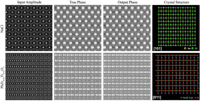
Figure 1. Example applications of a noise-removal DNN to instances of Poisson noise applied to 512×512 crops from TEM
images. Enlarged 64×64 regions from the top left of each crop are shown to ease comparison. This figure is adapted from our
earlier work72 under a Creative Commons Attribution 4.073 license.

often minimized by hardware. For example, by using aberration correctors136, 157–159 , choosing scanning transmission electron
microscopy (STEM) scan shapes and speeds that minimize distortions138 , and using stable sample holders to reduce drift160 .
Beam damage can also be reduced by using minimal electron voltage and electron dose161–163 , or dose-fractionation across
multiple frames in multi-pass transmission electron microscopy164–166 (TEM) or STEM167 .
    Deep learning is being applied to improve signal-to-noise for a variety of applications168–176 . Most approaches in electron
microscopy involve training ANNs to either map low-quality experimental177 , artificially deteriorated70, 178 or synthetic179–182
inputs to paired high-quality experimental measurements. For example, applications of a DNN trained with artificially
deteriorated TEM images are shown in figure 1. However, ANNs have also been trained with unpaired datasets of low-
quality and high-quality electron micrographs183 , or pairs of low-quality electron micrographs184, 185 . Another approach is
Noise2Void168 , ANNs are trained from single noisy images. However, Noise2Void removes information by masking noisy
input pixels corresponding to target output pixels. So far, most ANNs that improve electron microscope signal-to-noise have
been trained to decrease statistical noise70, 177, 179–181, 181–184, 186 as other approaches have been developed to correct electron
microscope scan distortions187, 188 and specimen drift141, 188, 189 . However, we anticipate that ANNs will be developed to correct
a variety of electron microscopy noise as ANNs have been developed for aberration correction of optical microscopy190–195 and
photoacoustic196 signals.

1.2 Compressed Sensing
Compressed sensing203–207 is the efficient reconstruction of a signal from a subset of measurements. Applications include faster
medical imaging208–210 , image compression211, 212 , increasing image resolution213, 214 , lower medical radiation exposure215–217 ,
and low-light vision218, 219 . In STEM, compressed sensing has enabled electron beam exposure and scan time to be decreased
by 10-100× with minimal information loss201, 202 . Thus, compressed sensing can be essential to investigations where the high
current density of electron probes damages specimens161, 220–226 . Even if the effects of beam damage can be corrected by
postprocessing, the damage to specimens is often permanent. Examples of beam-sensitive materials include organic crystals227 ,
metal-organic frameworks228 , nanotubes229 , and nanoparticle dispersions230 . In electron microscopy, compressed sensing is

                                                                                                                               2/98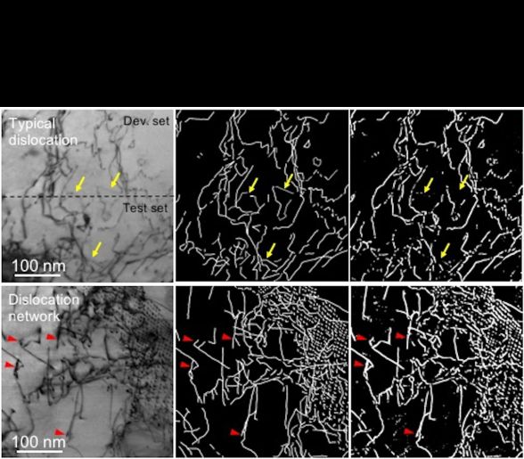
Figure 2. Example applications of DNNs to restore 512×512 STEM images from sparse signals. Training as part of a
generative adversarial network197–200 yields more realistic outputs than training a single DNN with mean squared errors.
Enlarged 64×64 regions from the top left of each crop are shown to ease comparison. a) Input is a Gaussian blurred 1/20
coverage spiral201 . b) Input is a 1/25 coverage grid202 . This figure is adapted from our earlier works under Creative Commons
Attribution 4.073 licenses.

especially effective due to high signal redundancy231 . For example, most electron microscopy images are sampled at 5-10×
their Nyquist rates232 to ease visual inspection, decrease sub-Nyquist aliasing233 , and avoid undersampling.
    Perhaps the most popular approach to compressed sensing is upsampling or infilling a uniformly spaced grid of signals234–236 .
Interpolation methods include Lancsoz234 , nearest neighbour237 , polynomial interpolation238 , Wiener239 and other resampling
methods240–242 . However, a variety of other strategies to minimize STEM beam damage have also been proposed, including
dose fractionation243 and a variety of sparse data collection methods244 . Perhaps the most intensively investigated approach
to the latter is sampling a random subset of pixels, followed by reconstruction using an inpainting algorithm244–249 . Random
sampling of pixels is nearly optimal for reconstruction by compressed sensing algorithms250 . However, random sampling
exceeds the design parameters of standard electron beam deflection systems, and can only be performed by collecting data
slowly138, 251 , or with the addition of a fast deflection or blanking system247, 252 .
    Sparse data collection methods that are more compatible with conventional STEM electron beam deflection systems
have also been investigated. For example, maintaining a linear fast scan deflection whilst using a widely-spaced slow scan
axis with some small random ‘jitter’245, 251 . However, even small jumps in electron beam position can lead to a significant
difference between nominal and actual beam positions in a fast scan. Such jumps can be avoided by driving functions with
continuous derivatives, such as those for spiral and Lissajous scan paths138, 201, 247, 253, 254 . Sang138, 254 considered a variety of
scans including Archimedes and Fermat spirals, and scans with constant angular or linear displacements, by driving electron
beam deflectors with a field-programmable gate array255 (FPGA) based system138 . Spirals with constant angular velocity
place the least demand on electron beam deflectors. However, dwell times, and therefore electron dose, decreases with radius.
Conversely, spirals created with constant spatial speeds are prone to systematic image distortions due to lags in deflector
responses. In practice, fixed doses are preferable as they simplify visual inspection and limit the dose dependence of STEM
noise129 .
    Deep learning can leverage an understanding of physics to infill images256–258 . Example applications include increasing
scanning electron microscopy178, 259, 260 (SEM), STEM202, 261 and TEM262 resolution, and infilling continuous sparse scans201 .
Example applications of DNNs to complete sparse spiral and grid scans are shown in figure 2. However, caution should be
used when infilling large regions as ANNs may generate artefacts if a signal is unpredictable201 . A popular alternative to deep
learning for infilling large regions is exemplar-based infilling263–266 . However, exemplar-based infilling often leaves artefacts267

                                                                                                                                 3/98
and is usually limited to leveraging information from single images. Smaller regions are often infilled by fast marching268 ,
Navier-Stokes infilling269 , or interpolation238 .

1.3 Labelling
Deep learning has been the basis of state-of-the-art classification270–273 since convolutional neural networks (CNNs) enabled a
breakthrough in classification accuracy on ImageNet71 . Most classifiers are single feedforward neural networks (FNNs) that
learn to predict discrete labels. In electron microscopy, applications include classifying image region quality274, 275 , material
structures276, 277 , and image resolution278 . However, siamese279–281 and dynamically parameterized282 networks can more
quickly learn to recognise images. Finally, labelling ANNs can learn to predict continuous features, such as mechanical
properties283 . Labelling ANNs are often combined with other methods. For example, ANNs can be used to automatically
identify particle locations186, 284–286 to ease subsequent processing.

Figure 3. Example applications of a semantic segmentation DNN to STEM images of steel to classify dislocation locations.
Yellow arrows mark uncommon dislocation lines with weak contrast, and red arrows indicate that fixed widths used for
dislocation lines are sometimes too narrow to cover defects. This figure is adapted with permission287 under a Creative
Commons Attribution 4.073 license.

1.4 Semantic Segmentation
Semantic segmentation is the classification of pixels into discrete categories. In electron microscopy, applications include the
automatic identification of local features288, 289 , such as defects290, 291 , dopants292 , material phases293 , material structures294, 295 ,
dynamic surface phenomena296 , and chemical phases in nanoparticles297 . Early approaches to semantic segmentation used
simple rules. However, such methods were not robust to a high variety of data298 . Subsequently, more adaptive algorithms
based on soft-computing299 and fuzzy algorithms300 were developed to use geometric shapes as priors. However, these methods
were limited by programmed features and struggled to handle the high variety of data.

                                                                                                                                        4/98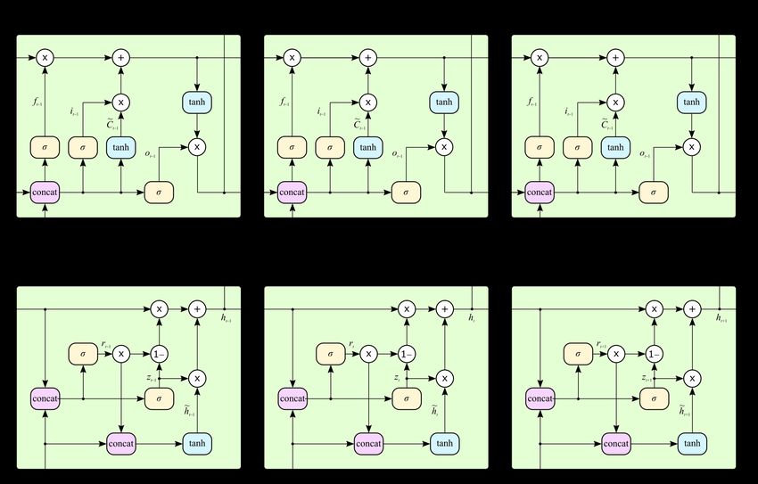
To improve performance, DNNs have been trained to semantically segment images301–308 . Semantic segmentation DNNs
have been developed for focused ion beam scanning electron microscopy309–311 (FIB-SEM), SEM311–314 , STEM287, 315 , and
TEM286, 310, 311, 316–319 . For example, applications of a DNN to semantic segmentation of STEM images of steel are shown in
figure 3. Deep learning based semantic segmentation also has a high variety of applications outside of electron microscopy,
including autonomous driving320–324 , dietary monitoring325, 326 , magnetic resonance images327–331 , medical images332–334 such
as prenatal ultrasound335–338 , and satellite image translation339–343 . Most DNNs for semantic segmentation are trained with
images segmented by humans. However, human labelling may be too expensive, time-consuming, or inappropriate for sensitive
data. Unsupervised semantic segmentation can avoid these difficulties by learning to segment images from an additional dataset
of segmented images344 or image-level labels345–348 . However, unsupervised semantic segmentation networks are often less
accurate than supervised networks.

Figure 4. Example applications of a DNN to reconstruct phases of exit wavefunction from intensities of single TEM images.
Phases in [−π, π) rad are depicted on a linear greyscale from black to white, and Miller indices label projection directions.
This figure is adapted from our earlier work349 under a Creative Commons Attribution 4.073 license.

1.5 Exit Wavefunction Reconstruction
Electrons exhibit wave-particle duality350, 351 , so electron propagation is often described by wave optics352 . Applications
of electron wavefunctions exiting materials353 include determining projected potentials and corresponding crystal structure
information354, 355 , information storage, point spread function deconvolution, improving contrast, aberration correction356 ,
thickness measurement357 , and electric and magnetic structure determination358, 359 . Usually, exit wavefunctions are either
iteratively reconstructed from focal series360–364 or recorded by electron holography352, 363, 365 . However, iterative reconstruction
is often too slow for live applications, and holography is sensitive to distortions and may require expensive microscope
modification.
    Non-iterative methods based on DNNs have been developed to reconstruct optical exit wavefunctions from focal series69 or
single images366–368 . Subsequently, DNNs have been developed to reconstruct exit wavefunctions from single TEM images349 ,
as shown in figure 4. Indeed, deep learning is increasingly being applied to accelerated quantum mechanics369–374 . Other
examples of DNNs adding new dimensions to data include semantic segmentation described in section 1.4, and reconstructing
3D atomic distortions from 2D images375 . Non-iterative methods that do not use ANNs to recover phase information from
single images have also been developed376, 377 . However, they are limited to defocused images in the Fresnel regime376 , or to
non-planar incident wavefunctions in the Fraunhofer regime377 .

                                                                                                                                5/98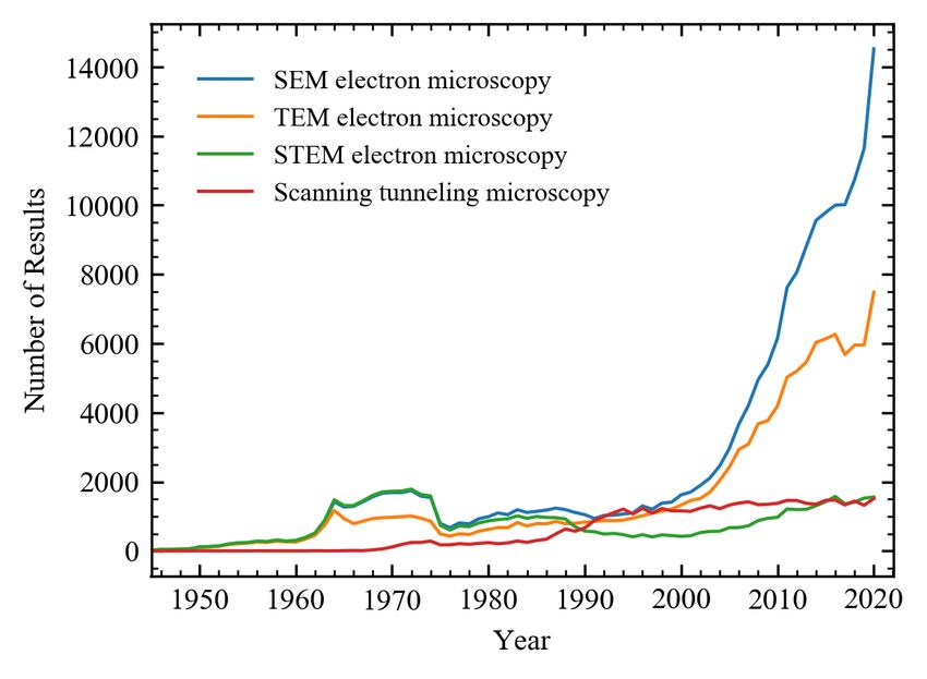
2 Resources
Access to scientific resources is essential to scientific enterprise378 . Fortunately, most resources needed to get started with
machine learning are freely available. This section provides directions to various machine learning resources, including how to
access deep learning frameworks, a free GPU or tensor processing unit (TPU) to accelerate tensor computations, platforms
that host datasets and source code, and pretrained models. To support the ideals of open science embodied by Plan S378–380 ,
we focus on resources that enhance collaboration and enable open access381 . We also discuss how electron microscopes can
interface with ANNs and the importance of machine learning resources in the context of electron microscopy. However, we
expect that our insights into electron microscopy can be generalized to other scientific fields.

2.1 Hardware Acceleration
A DNN is an ANN with multiple layers that perform a sequence of tensor operations. Tensors can either be computed on central
processing units (CPUs) or hardware accelerators62 , such as FPGAs382–385 , GPUs386–388 , and TPUs389–391 . Most benchmarks
indicate that GPUs and TPUs outperform CPUs for typical DNNs that could be used for image processing392–396 in electron
microscopy. However, GPU and CPU performance can be comparable when CPU computation is optimized397 . TPUs often
outperform GPUs394 , and FPGAs can outperform GPUs398, 399 if FPGAs have sufficient arithmetic units400, 401 . Typical power
consumption per TFLOPS402 decreases in order CPU, GPU, FPGA, then TPU, so hardware acceleration can help to minimize
long-term costs and environmental damage403 .
    For beginners, Google Colab404–407 and Kaggle408 provide hardware accelerators in ready-to-go deep learning environments.
Free compute time on these platforms is limited as they are not intended for industrial applications. Nevertheless, the free
compute time is sufficient for some research409 . For more intensive applications, it may be necessary to get permanent access
to hardware accelerators. If so, many online guides detail how to install410, 411 and set up an Nvidia412 or AMD413 GPU in
a desktop computer for deep learning. However, most hardware comparisons for deep learning414 focus on Nvidia GPUs as
most deep learning frameworks use Nvidia’s proprietary Compute Unified Device Architecture (CUDA) Deep Neural Network
(cuDNN) primitives for deep learning415 , which are optimized for Nvidia GPUs. Alternatively, hardware accelerators may be
accessible from a university or other institutional high performance computing (HPC) centre, or via a public cloud service
provider416–419 .
               Framework             License                                          Programming Interfaces
Apache SINGA420                   Apache 2.0421    C++, Java, Python
BigDL422                          Apache 2.0423    Python, Scala
Caffe424, 425                     BSD426           C++, MATLAB, Python
Chainer427                        MIT428           Python
Deeplearning4j429                 Apache 2.0430    Clojure, Java, Kotlin, Python, Scala
Dlib431, 432                      BSL433           C++
Flux434                           MIT435           Julia
MATLAB Deep Learning Toolbox436   Proprietary437   MATLAB
Microsoft Cognitive Toolkit438    MIT439           BrainScript, C++, Python
Apache MXNet440                   Apache 2.0441    C++, Clojure, Go, JavaScript, Julia, Matlab, Perl, Python, R, Scala
OpenNN442                         GNU LGPL443      C++
PaddlePaddle444                   Apache 2.0445    C++
PyTorch446                        BSD447           C++, Python
TensorFlow448, 449                Apache 2.0450    C++, C#, Go, Haskell, Julia, MATLAB, Python, Java, JavaScript, R, Ruby, Rust, Scala, Swift
Theano451, 452                    BSD453           Python
Torch454                          BSD455           C, Lua
Wolfram Mathematica456            Proprietary457   Wolfram Language

Table 1. Deep learning frameworks with programming interfaces. Most frameworks have open source code and many support
multiple programming languages.

2.2 Deep Learning Frameworks
A deep learning framework9, 458–464 (DLF) is an interface, library or tool for DNN development. Features often include automatic
differentiation465 , heterogeneous computing, pretrained models, and efficient computing466 with CUDA467–469 , cuDNN415, 470 ,
OpenMP471, 472 , or similar libraries. Popular DLFs tabulated in table 1 often have open source code and support multiple
programming interfaces. Overall, TensorFlow448, 449 is the most popular DLF473 . However, PyTorch446 is the most popular DLF
at top machine learning conferences473, 474 . Some DLFs also have extensions that ease development or extend functionality. For
example, TensorFlow extensions475 that ease development include Keras476 , Sonnet477 , Tensor2Tensor478 and TFLearn479, 480 ,
and extensions that add functionality include Addons481 , Agents482 , Dopamine483 , Federated484–486 , Probability487 , and
TRFL488 . In addition, DLFs are supplemented by libraries for predictive data analysis, such as scikit-learn489 .

                                                                                                                                         6/98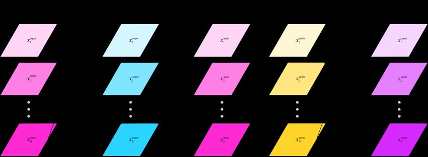
A limitation of the DLFs in table 1 is that users must use programming interfaces. This is problematic as many electron
microscopists have limited, if any, programming experience. To increase accessibility, a range of graphical user interfaces (GUIs)
have been created for ANN development. For example, ANNdotNET490 , Create ML491 , Deep Cognition492 , Deep Network
Designer493 , DIGITS494 , ENNUI495 , Expresso496 , Neural Designer497 , Waikato Environment for Knowledge Analysis498–500
(WEKA) and ZeroCostDL4Mic501 . The GUIs offer less functionality and scope for customization than programming interfaces.
However, GUI-based DLFs are rapidly improving. Moreover, existing GUI functionality is more than sufficient to implement
popular FNNs, such as image classifiers272 and encoder-decoders305–308, 502–504 .

2.3 Pretrained Models
Training ANNs is often time-consuming and computationally expensive403 . Fortunately, pretrained models are available from a
range of open access collections505 , such as Model Zoo506 , Open Neural Network Exchange507–510 (ONNX) Model Zoo511 ,
TensorFlow Hub512, 513 , and TensorFlow Model Garden514 . Some researchers also provide pretrained models via project
repositories70, 201, 202, 231, 349 . Pretrained models can be used immediately or to transfer learning515–521 to new applications. For
example, by fine-tuning and augmenting the final layer of a pretrained model522 . Benefits of transfer learning can include
decreasing training time by orders of magnitude, reducing training data requirements, and improving generalization520, 523 .
    Using pretrained models is complicated by ANNs being developed with a variety of DLFs in a range of programming
languages. However, most DLFs support interoperability. For example, by supporting the saving of models to a common format
or to formats that are interoperable with the Neural Network Exchange Format524 (NNEF) or ONNX formats. Many DLFs
also support saving models to HDF5525, 526 , which is popular in the pycroscopy527, 528 and HyperSpy529, 530 libraries used by
electron microscopists. The main limitation of interoperability is that different DLFs may not support the same functionality.
For example, Dlib431, 432 does not support recurrent neural networks531–536 (RNNs).

2.4 Datasets
Randomly initialized ANNs537 must be trained, validated, and tested with large, carefully partitioned datasets to ensure that
they are robust to general use538 . Most ANN training starts from random initialization, rather than transfer learning515–521 , as:

   1. Researchers may be investigating modifications to ANN architecture or ability to learn.

   2. Pretrained models may be unavailable or too difficult to find.

   3. Models may quickly achieve sufficient performance from random initialization. For example, training an encoder-decoder
      based on Xception539 to improve electron micrograph signal-to-noise70 can require less training than for PASCAL VOC
      2012540 semantic segmentation305 .

   4. There may be a high computing budget, so transfer learning is unnecessary541, 542 .

There are millions of open access datasets543, 544 and a range of platforms that host545–549 or aggregate550–553 machine learning
datasets. Openly archiving datasets drives scientific enterprise by reducing need to repeat experiments554–558 , enabling new
applications through data mining559, 560 , and standardizing performance benchmarks561 . For example, popular datasets used to
standardize image classification performance benchmarks include CIFAR-10562, 563 , MNIST564 and ImageNet565 . A high range
of both domain-specific and general platforms that host scientific data for free are listed by the Open Access Directory566 and
Nature Scientific Data567 . For beginners, we recommend Zenodo568 as it is free, open access, has an easy-to-use interface, and
will host an unlimited number of datasets smaller than 50 GB for at least 20 years569 .
    There are a range of platforms dedicated to hosting electron microscopy datasets, including the Caltech Electron Tomography
Database570 (ETDB-Caltech), Electron Microscopy Data Bank571–576 (EMDataBank), and the Electron Microscopy Public
Image Archive577 (EMPIAR). However, most electron microscopy datasets are small, esoteric or are not partitioned for
machine learning231 . Nevertheless, a variety of large machine learning datasets for electron microscopy are being published in
independent repositories231, 578, 579 , including Warwick Electron Microscopy Datasets231 (WEMD) that we curated. In addition,
a variety of databases host information that supports electron microscopy. For example, crystal structure databases provide data
in standard formats580, 581 , such as Crystallography Information Files582–585 (CIFs). Large crystal structure databases586–588
containing over 105 crystal structures include the Crystallography Open Database589–594 (COD), Inorganic Crystal Structure
Database595–599 (ICSD), and National Institute of Standards and Technology (NIST) Crystal Data600, 601 .
    To achieve high performance, it may be necessary to curate a large dataset for ANN training2 . However, large datasets
like DeepMind Kinetics602 , ImageNet565 , and YouTube 8M603 may take a team months to prepare. As a result, it may not be
practical to divert sufficient staff and resources to curate a high-quality dataset, even if curation is partially automated603–610 .
To curate data, human capital can be temporarily and cheaply increased by using microjob services611 . For example, through
microjob platforms tabulated in table 2. Increasingly, platforms are emerging that specialize in data preparation for machine

                                                                                                                                7/98
Platform Website For Machine Learning
Amazon Mechanical Turk https://www.mturk.com General tasks
Appen https://appen.com Machine learning data preparation
Clickworker https://www.clickworker.com Machine learning data preparation
Fiverr https://www.fiverr.com General tasks
Hive https://thehive.ai Machine learning data preparation
iMerit https://imerit.net Machine learning data preparation
JobBoy https://www.jobboy.com General tasks
Minijobz https://minijobz.com General tasks
Microworkers https://www.microworkers.com General tasks
OneSpace https://freelance.onespace.com General tasks
Playment https://playment.io Machine learning data preparation
RapidWorkers https://rapidworkers.com General tasks
Scale https://scale.com Machine learning data preparation
Smart Crowd https://thesmartcrowd.lionbridge.com General tasks
Trainingset.ai https://www.trainingset.ai Machine learning data preparation
ySense https://www.ysense.com General tasks
Table 2. Microjob service platforms. The size of typical tasks varies for different platforms and some platforms specialize in
preparing machine learning datasets.
learning. Nevertheless, microjob services may be inappropriate for sensitive data or tasks that require substantial domain-specific
knowledge.
2.5 Source Code
Software is part of our cultural, industrial, and scientific heritage612 . Source code should therefore be archived where
possible. For example, on an open source code platform such as Apache Allura613 , AWS CodeCommit614 , Beanstalk615 ,
BitBucket616 , GitHub617 , GitLab618 , Gogs619 , Google Cloud Source Repositories620 , Launchpad621 , Phabricator622 , Savan-
nah623 or SourceForge624 . These platforms enhance collaboration with functionality that helps users to watch625 and contribute
improvements626–632 to source code. The choice of platform is often not immediately important for small electron microscopy
projects as most platforms offer similar functionality. Nevertheless, functionality comparisons of open source platforms
are available633–635 . For beginners, we recommend GitHub as it is actively developed, scalable to large projects and has an
easy-to-use interface.
2.6 Finding Information
Most web traffic636, 637 goes to large-scale web search engines638–642 such as Bing, DuckDuckGo, Google, and Yahoo.
This includes searches for scholarly content643–645 . We recommend Google for electron microscopy queries as it appears
to yield the best results for general646–648 , scholarly644, 645 and other649 queries. However, general search engines can be
outperformed by dedicated search engines for specialized applications. For example, for finding academic literature650–652 ,
data653 , jobs654, 655 , publication venues656 , patents657–660 , people661–663 , and many other resources. The use of search engines
is increasingly political664–666 as they influence which information people see. However, most users appear to be satisfied with
their performance667 .
Introductory textbooks are outdated668, 669 insofar that most information is readily available online. We find that some
websites are frequent references for up-to-date and practical information:
1. Stack Overflow670–675 is a source of working code snippets and a useful reference when debugging code.
2. Papers With Code State-of-the-Art561 leaderboards rank the highest performing ANNs with open source code for various
benchmarks.
3. Medium676 and its subsidiaries publish blogs with up-to-date and practical advice about machine learning.
4. The Machine Learning subreddit677 hosts discussions about machine learning. In addition, there is a Learn Machine
Learning subreddit678 aimed at beginners.
5. Dave Mitchell’s DigitalMicrograph Scripting Website679, 680 hosts a collection of scripts and documentation for program-
ming electron microscopes.
6. The Internet Archive681, 682 maintains copies of software and media, including webpages via its Wayback Machine683–685 .
8/987. Distill686 is a journal dedicated to providing clear explanations about machine learning. Monetary prizes are awarded for
excellent communication and refinement of ideas.
This list enumerates popular resources that we find useful, so it may introduce personal bias. However, alternative guides
to useful resources are available687–689 . We find that the most common issues finding information are part of an ongoing
reproducibility crisis690, 691 where machine learning researchers do not publish their source code or data. Nevertheless, third
party source code is sometimes available. Alternatively, ANNs can reconstruct source code from some research papers692 .
2.7 Scientific Publishing
The number of articles published per year in reputable peer-reviewed693–697 scientific journals698, 699 has roughly doubled
every nine years since the beginning of modern science700 . There are now over 25000 peer-reviewed journals699 with varying
impact factors701–703 , scopes and editorial policies. Strategies to find the best journal to publish in include using online journal
finders704 , seeking the advice of learned colleagues, and considering where similar research has been published. Increasingly,
working papers are also being published in open access preprint archives705–707 . For example, the arXiv708, 709 is a popular
preprint archive for computer science, mathematics, and physics. Advantages of preprints include ensuring that research is
openly available, increasing discovery and citations710–714 , inviting timely scientific discussion, and raising awareness to reduce
unnecessary duplication of research. Many publishers have adapted to the popularity of preprints705 by offering open access
publication options715–718 and allowing, and in some cases encouraging719 , the prior publication of preprints. Indeed, some
journals are now using the arXiv to host their publications720 .
A variety of software can help authors prepare scientific manuscripts721 . However, we think the most essential software
is a document preparation system. Most manuscripts are prepared with Microsoft Word722 or similar software723 . However,
Latex724–726 is a popular alternative among computer scientists, mathematicians and physicists727 . Most electron microscopists
at the University of Warwick appear to prefer Word. A 2014 comparison of Latex and Word found that Word is better at all
tasks other than typesetting equations728 . However, in 2017 it become possible to use Latex to typeset equations within Word727 .
As a result, Word appears to be more efficient than Latex for most manuscript preparation. Nevertheless, Latex may still be
preferable to authors who want fine control over typesetting729, 730 . As a compromise, we use Overleaf731 to edit Latex source
code, then copy our code to Word as part of proofreading to identify issues with grammar and wording.
Figure 5. Reciprocity of TEM and STEM electron optics.
9/983 Electron Microscopy
An electron microscope is an instrument that uses electrons as a source of illumination to enable the study of small objects.
Electron microscopy competes with a large range of alternative techniques for material analysis732–734 , including atomic force
microscopy735–737 (AFM); Fourier transformed infrared (FTIR) spectroscopy738, 739 ; nuclear magnetic resonance740–743 (NMR);
Raman spectroscopy744–750 ; and x-ray diffraction751, 752 (XRD), dispersion753 , fluorescence754, 755 (XRF), and photoelectron
spectroscopy756, 757 (XPS). Quantitative advantages of electron microscopes can include higher resolution and depth of field,
and lower radiation damage than light microscopes758 . In addition, electron microscopes can record images, enabling visual
interpretation of complex structures that may otherwise be intractable. This section will briefly introduce varieties of electron
microscopes, simulation software, and how electron microscopes can interface with ANNs.
3.1 Microscopes
Figure 6. Numbers of results per year returned by Dimensions.ai abstract searches for SEM, TEM, STEM, STM and REM
qualitate their popularities. The number of results for 2020 is extrapolated using the mean rate before 14th July 2020.
There are a variety of electron microscopes that use different illumination mechanisms. For example, reflection electron
microscopy759, 760 (REM), scanning electron microscopy761, 762 (SEM), scanning transmission electron microscopy763, 764
(STEM), scanning tunnelling microscopy765, 766 (STM), and transmission electron microscopy767–769 (TEM). To roughly
gauge popularities of electron microscope varieties, we performed abstract searches with Dimenions.ai651, 770–772 for their
abbreviations followed by “electron microscopy” e.g. “REM electron microscopy”. Numbers of results per year in figure 6
qualitate that popularity increases in order REM, STM, STEM, TEM, then SEM. It may be tempting to attribute the popularity
of SEM over TEM to the lower cost of SEM773 , which increases accessibility. However, a range of considerations influence the
procurement of electron microscopes774 and hourly pricing at universities775–779 is similar for SEM and TEM.
In SEM, material surfaces are scanned by sequential probing with a beam of electrons, which are typically accelerated
to 0.2-40 keV. The SEM detects quanta emitted from where the beam interacts with the sample. Most SEM imaging uses
low-energy secondary electrons. However, reflection electron microscopy759, 760 (REM) uses elastically backscattered electrons
and is often complimented by a combination of reflection high-energy electron diffraction780–782 (RHEED), reflection high-
energy electron loss spectroscopy783, 784 (RHEELS) and spin-polarized low-energy electron microscopy785–787 (SPLEEM).
Some SEMs also detect Auger electrons788, 789 . To enhance materials characterization, most SEMs also detect light. The most
common light detectors are for cathodoluminescence and energy dispersive r-ray790, 791 (EDX) spectroscopy. Nonetheless,
some SEMs also detect Bremsstrahlung radiation792 .
Alternatively, TEM and STEM detect electrons transmitted through specimens. In conventional TEM, a single region is
exposed to a broad electron beam. In contrast, STEM uses a fine electron beam to probe a series of discrete probing locations.
Typically, electrons are accelerated across a potential difference to kinetic energies, Ek , of 80-300 keV. Electrons also have rest
energy Ee = me c2 , where me is electron rest mass and c is the speed of light. The total energy, Et = Ee + Ek , of free electrons is
10/98related to their rest mass energy by a Lorentz factor, γ,
Et = γme c2 , (1)
γ = (1 − v2 /c2 )1/2 , (2)
where v is the speed of electron propagation in the rest frame of an electron microscope. Electron kinetic energies in TEM and
STEM are comparable to their rest energy, Ee = 511 keV793 , so relativistic phenomena794, 795 must be considered to accurately
describe their dynamics.
Electrons exhibit wave-particle duality350, 351 . Thus, in an ideal electron microscope, the maximum possible detection angle,
θ , between two point sources separated by a distance, d, perpendicular to the electron propagation direction is diffraction-limited.
The resolution limit for imaging can be quantified by Rayleigh’s criterion796–798
λ
θ ' 1.22 , (3)
d
where resolution increases with decreasing wavelength, λ . Electron wavelength decreases with increasing accelerating voltage,
as described by the relativistic de Broglie relation799–801 ,
−1/2
λ = hc Ek2 + 2Ee Ek , (4)
where h is Planck’s constant793 . Electron wavelengths for typical acceleration voltages tabulated by JEOL are in picometres802 .
In comparison, Cu K-α x-rays, which are often used for XRD, have wavelengths near 0.15 nm803 . In theory, electrons can
therefore achieve over 100× higher resolution than x-rays. Electrons and x-rays are both ionizing; however, electrons often
do less radiation damage to thin specimens than x-rays758 . Tangentially, TEM and STEM often achieve over 10 times higher
resolution than SEM804 as transmitted electrons in TEM and STEM are easier to resolve than electrons returned from material
surfaces in SEM.
In practice, TEM and STEM are also limited by incoherence805–807 introduced by inelastic scattering, electron energy
spread, and other mechanisms. TEM and STEM are related by an extension of Helmholtz reciprocity808, 809 where the source
plane in a TEM corresponds to the detector plane in a STEM810 , as shown in figure 5. Consequently, TEM coherence is limited
by electron optics between the specimen and image, whereas STEM coherence is limited by the illumination system. For
conventional TEM and STEM imaging, electrons are normally incident on a specimen811 . Advantages of STEM imaging can
include higher contrast and resolution than TEM imaging, and lower radiation damage812 . As a result, STEM is increasing
being favoured over TEM for high-resolution studies. However, we caution that definitions of TEM and STEM resolution can
be disparate813 .
In addition to conventional imaging, TEM and STEM include a variety of operating modes for different applications.
For example, TEM operating configurations include electron diffraction814 ; convergent beam electron diffraction815–817
(CBED); tomography818–826 ; and bright field768, 827–829 , dark field768, 829 and annular dark field830 imaging. Similarly, STEM
operating configurations include differential phase contrast831–834 ; tomography818, 820, 822, 823 ; and bright field835, 836 or dark
field837 imaging. Further, electron cameras838, 839 are often supplemented by secondary signal detectors. For example,
elemental composition is often mapped by EDX spectroscopy, electron energy loss spectroscopy840, 841 (EELS) or wavelength
dispersive spectroscopy842, 843 (WDS). Similarly, electron backscatter diffraction844–846 (EBSD) can detect strain847–849 and
crystallization850–852 .
3.2 Contrast Simulation
The propagation of electron wavefunctions though electron microscopes can be described by wave optics136 . Further, the most
popular approach to modelling measurement contrast is multislice simulation853, 854 , where an electron wavefunction is itera-
tively perturbed as it travels through a model of a specimen. Multislice software for electron microscopy includes ACEM854–856 ,
clTEM857, 858 , cudaEM859 , Dr. Probe860, 861 , EMSoft862, 863 , JEMS864 , JMULTIS865 , MULTEM866–868 , NCEMSS869, 870 , NU-
MIS871 , Prismatic872–874 , QSTEM875 , SimulaTEM876 , STEM-CELL877 , Tempas878 , and xHREM879–884 . We find that most
multislice software is a recreation and slight modification of common functionality, possibly due to a publish-or-perish culture
in academia885–887 . Bloch-wave simulation854, 888–892 is an alternative to multislice simulation that can reduce computation
time and memory requirements for crystalline materials893 .
3.3 Automation
Most modern electron microscopes support Gatan Microscopy Suite (GMS) Software894 . GMS enables electron microscopes to
be programmed by DigitalMicrograph Scripting, a propriety Gatan programming language akin to a simplified version of C++.
11/98A variety of DigitalMicrograph scripts, tutorials and related resources are available from Dave Mitchell’s DigitalMicrograph
Scripting Website679, 680 , FELMI/ZFE’s Script Database895 and Gatan’s Script library896 . Some electron microscopists also
provide DigitalMicrograph scripting resources on their webpages897–899 . However, DigitalMicrograph scripts are slow insofar
that they are interpreted at runtime, and there is limited native functionality for parallel and distributed computing. As a result,
extensions to DigitalMicrograph scripting are often developed in other programming languages that offer more functionality.
Historically, most extensions were developed in C++900 . This was problematic as there is limited documentation, the
standard approach used outdated C++ software development kits such as Visual Studio 2008, and programming expertise
required to create functions that interface with DigitalMicrograph scripts limited accessibility. To increase accessibility, recent
versions of GMS now support python901 . This is convenient as it enables ANNs developed with python to readily interface with
electron microscopes. For ANNs developed with C++, users have the option to either create C++ bindings for DigitalMicrograph
script or for python. Integrating ANNs developed in other programming languages is more complicated as DigitalMicrograph
provides almost no support. However, that complexity can be avoided by exchanging files from DigitalMicrograph script to
external libraries via a random access memory (RAM) disk902 or secondary storage903 .
Increasing accessibility, there are collections of GMS plugins with GUIs for automation and analysis897–899, 904 . In addition,
various individual plugins are available905–909 . Some plugins are open source, so they can be adapted to interface with ANNs.
However, many high-quality plugins are proprietary and closed source, limiting their use to automation of data collection and
processing. Plugins can also be supplemented by a variety of libraries and interfaces for electron microscopy signal processing.
For example, popular general-purpose software includes ImageJ910 , pycroscopy527, 528 and HyperSpy529, 530 . In addition, there
are directories for tens of general-purpose and specific electron microscopy programs911–913 .
4 Components
Most modern ANNs are configured from a variety of DLF components. To take advantage of hardware accelerators62 , most
ANNs are implemented as sequences of parallelizable layers of tensor operations914 . Layers are often parallelized across
data and may be parallelized across other dimensions915 . This section introduces popular nonlinear activation functions,
normalization layers, convolutional layers, and skip connections. To add insight, we provide comparative discussion and
address some common causes of confusion.
4.1 Nonlinear Activation
In general, DNNs need multiple layers to be universal approximators37–45 . Nonlinear activation functions916, 917 are therefore
essential to DNNs as successive linear layers can be contracted to a single layer. Activation functions separate artificial neurons,
similar to biological neurons918 . To learn efficiently, most DNNs are tens or hundreds of layers deep47, 919–921 . High depth
increases representational capacity47 , which can help training by gradient descent as DNNs evolve as linear models922 and
nonlinearities can create suboptimal local minima where data cannot be fit by linear models923 . There are infinitely many
possible activation functions. However, most activation functions have low polynomial order, similar to physical Hamiltonians47 .
Most ANNs developed for electron microscopy are for image processing, where the most popular nonlinearities are rectifier
linear units924, 925 (ReLUs). The ReLU activation, f (x), of an input, x, and its gradient, ∂x f (x), are
(
f (x) = max(0, x) (5a) ∂ f (x) 0, if x ≤ 0
= (5b)
∂x 1, if x > 0
Popular variants of ReLUs include Leaky ReLU926 ,
(
f (x) = max(αx, x) (6a) ∂ f (x) α, if x ≤ 0
= (6b)
∂x 1, if x > 0
where α is a hyperparameter, parametric ReLU22 (PreLU) where α is a learned parameter, dynamic ReLU where α is a learned
function of inputs927 , and randomized leaky ReLU928 (RReLU) where α is chosen randomly. Typically, learned PreLU α are
higher the nearer a layer is to ANN inputs22 . Motivated by limited comparisons that do not show a clear performance difference
between ReLU and leaky ReLU929 , some blogs930 argue against using leaky ReLU due to its higher computational requirements
and complexity. However, an in-depth comparison found that leaky ReLU variants consistently slightly outperform ReLU928 . In
addition, the non-zero gradient of leaky ReLU for x ≤ 0 prevents saturating, or “dying”, ReLU931–933 , where the zero gradient
of ReLUs stops learning.
12/98There are a variety of other piecewise linear ReLU variants that can improve performance. For example, ReLUh activations
are limited to a threshold934 , h, so that
0, if x ≤ 0
f (x) = min(max(0, x), h) (7a) ∂ f (x)
= 1, if 0 < x ≤ h (7b)
∂x
0, if x > h
Thresholds near h = 6 are often effective, so popular choice is ReLU6. Another popular activation is concatenated ReLU935
(CReLU), which is the concatenation of ReLU(x) and ReLU(−x). Other ReLU variants include adaptive convolutional936 ,
bipolar937 , elastic938 , and Lipschitz939 ReLUs. However, most ReLU variants are uncommon as they are more complicated
than ReLU and offer small, inconsistent, or unclear performance gains. Moreover, it follows from the universal approximator
theorems37–45 that disparity between ReLU and its variants approaches zero as network depth increases.
In shallow networks, curved activation functions with non-zero Hessians often accelerate convergence and improve
performance. A popular activation is the exponential linear unit940 (ELU),
( (
α(exp(x) − 1), if x ≤ 0 ∂ f (x) α exp(x), if x ≤ 0
f (x) = (8a) = (8b)
x, if x ≥ 0 ∂x 1, if x ≥ 0
where α is a learned parameter. Further, a scaled ELU941 (SELU),
( (
λ α(exp(x) − 1), if x ≤ 0 ∂ f (x) λ α exp(x), if x ≤ 0
f (x) = (9a) = (9b)
λ x, if x ≥ 0 ∂x λ, if x ≥ 0
with fixed α = 1.67326 and scale factor λ = 1.0507 can be used to create self-normalizing neural networks (SNNs). A SNN
cannot be derived from ReLUs or most other activation functions. Activation functions with curvature are especially common
in ANNs with only a couple of layers. For example, activation functions in radial basis function (RBF) networks942–945 , which
are efficient universal approximators, are often Gaussians, multiquadratics, inverse multiquadratics, or square-based RBFs946 .
Similarly, support vector machines947–949 (SVMs) often use RBFs, or sigmoids,
1 ∂ f (x)
f (x) = (10a) = f (x) (1 − f (x)) (10b)
1 + exp(−x) ∂x
Sigmoids can also be applied to limit the support of outputs. Unscaled, or “logistic”, sigmoids are often denoted σ (x) and are
related to tanh by tanh(x) = 2σ (2x) − 1. To avoid expensive exp(−x) in the computation of tanh, we recommend K-tanH950 ,
LeCun tanh951 , or piecewise linear approximation952, 953 .
The activation functions introduced so far are scalar functions than can be efficiently computed in parallel for each input
element. However, functions of vectors, x = {x1 , x2 , ...}, are also popular. For example, softmax activation954 ,
exp(x) f (x)
f (x) = (11a) = ∑ f (x)i (δi j − f (x) j ) (11b)
sum(exp(x)) ∂xj i
is often applied before computing cross-entropy losses for classification networks. Similarly, Ln vector normalization,
x xnj
f (x) = (12a) f (x) 1
||x||n = 1− (12b)
∂xj ||x||n ||x||nn
with n = 2 is often applied to vectors to ensure that they lie on a unit sphere349 . Finally, max pooling955, 956 ,
13/98(
f (x) = max(x) (13a) f (x) 1, if j = argmax(x)
= (13b)
∂xj 0, if j 6= argmax(x)
is another popular multivariate activation function that is often used for downsampling. However, max pooling has fallen out
of favour as it is often outperformed by strided convolutional layers957 . Other vector activation functions include squashing
nonlinearities for dynamic routing by agreement in capsule networks958 and cosine similarity959 .
There are many other activation functions that are not detailed here for brevity. Further, finding new activation functions
is an active area of research960, 961 . Notable variants include choosing activation functions from a set before training962, 963
and learning activation functions962, 964–967 . Activation functions can also encode probability distributions968–970 or include
noise953 . Finally, there are a variety of other deterministic activation functions961, 971 . In electron microscopy, most ANNs
enable new or enhance existing applications. Subsequently, we recommend using computationally efficient and established
activation functions unless there is a compelling reason to use a specialized activation function.
4.2 Normalization
Normalization972–974 standardizes signals, which can accelerate convergence by gradient descent and improve performance.
Batch normalization975–980 is the most popular normalization layer in image processing DNNs trained with minibatches of N
examples. Technically, a “batch” is an entire training dataset and a “minibatch” is a subset; however, the “mini” is often omitted
where meaning is clear from context. During training, batch normalization applies a transform,
1 N
µB = ∑ xi , (14)
N i=1
1 N
σB2 = ∑ (xi − µB )2 , (15)
N i=1
x − µB
x̂ = 2 , (16)
(σB + ε)1/2
BatchNorm(x) = γ x̂ + β , (17)
where x = {x1 , ..., xN } is a batch of layer inputs, γ and β are a learnable scale and shift, and ε is a small constant added for
numerical stability. During inference, batch normalization applies a transform,
γ γE[x]
BatchNorm(x) = x + β − , (18)
(Var[x] + ε)1/2 (Var[x] + ε)1/2
where E[x] and Var[x] are expected batch means and variances. For convenience, E[x] and Var[x] are often estimated with
exponential moving averages that are tracked during training. However, E[x] and Var[x] can also be estimated by propagating
examples through an ANN after training.
Increasing batch size stabilizes learning by averaging destabilizing loss spikes over batches261 . Batched learning also
enables more efficient utilization of modern hardware accelerators. For example, larger batch sizes improve utilization of
GPU memory bandwidth and throughput391, 981, 982 . Using large batches can also be more efficient than many small batches
when distributing training across multiple CPU clusters or GPUs due to communication overheads. However, the performance
benefits of large batch sizes can come at the cost of lower test accuracy as training with large batches tends to converge to
sharper minima983, 984 . As a result, it is often best not to use batch sizes higher than N ≈ 32 for image classification985 . However,
learning rate scaling541 and layer-wise adaptive learning rates986 can increase accuracy of training with fixed larger batch sizes.
Batch size can also be increased throughout training without compromising accuracy987 to exploit effective learning rates being
inversely proportional to batch size541, 987 . Alternatively, accuracy can be improved by creating larger batches from replicated
instances of training inputs with different data augmentations988 .
There are a few caveats to batch normalization. Originally, batch normalization was applied before activation976 . However,
applying batch normalization after activation often slightly improves performance989, 990 . In addition, training can be sensitive
to the often-forgotten ε hyperparameter991 in equation 16. Typically, performance decreases as ε is increased above ε ≈ 0.001;
however, there is a sharp increase in performance around ε = 0.01 on ImageNet. Finally, it is often assumed that batches
are representative of the training dataset. This is often approximated by shuffling training data to sample independent and
identically distributed (i.i.d.) samples. However, performance can often be improved by prioritizing sampling992, 993 . We
observe that batch normalization is usually effective if batch moments, µB and σB , have similar values for every batch.
14/98Batch normalization is less effective when training batch sizes are small, or do not consist of independent samples. To
improve performance, standard moments in equation 16 can be renormalized994 to expected means, µ, and standard deviations,
σ,
x̂ ← rx̂ + d , (19)
σ
B
r = clip[1/rmax ,rmax ] , (20)
σ
µB − µ
d = clip[−dmax ,dmax ] , (21)
σ
where gradients are not backpropagated with respect to (w.r.t.) the renormalization parameters, r and d. Moments, µ and σ are
tracked by exponential moving averages and clipping to rmax and dmax improves learning stability. Usually, clipping values
are increased from starting values of rmax = 1 and dmax = 0, which correspond to batch normalization, as training progresses.
Another approach is virtual batch normalization995 (VBN), which estimates µ and σ from a reference batch of samples and
does not require clipping. However, VBN is computationally expensive as it requires computing a second batch of statistics at
every training iteration. Finally, online996 and streaming974 normalization enable training with small batch sizes by replace µB
and σB in equation 16 with their exponential moving averages.
There are alternatives to the L2 batch normalization of equations 14-18 that standardize to different Euclidean norms. For
example, L1 batch normalization997 computes
1 N
s1 = ∑ |xi − µB | ,
N i=1
(22)
x − µB
x̂ = , (23)
CL1 s1
where CL1 = (π/2)1/2 . Although the CL1 factor could be learned by ANN parameters, its inclusion accelerates convergence of
the original implementation of L1 batch normalization997 . Another alternative is L∞ batch normalization997 , which computes
s∞ = mean(topk (|x − µB |)) , (24)
x − µB
x̂ = , (25)
CL∞ s∞
where CL∞ is a scale factor, and topk (x) returns the k highest elements of x. Hoffer et al suggest k = 10997 . Some L1 batch
normalization proponents claim that L1 batch normalization outperforms975 or achieves similar performance997 to L2 batch
normalization. However, we found that L1 batch normalization often lowers performance in our experiments. Similarly, L∞
batch normalization often lowers performance997 . Overall, L1 and L∞ batch normalization do not appear to offer a substantial
advantage over L2 batch normalization.
Figure 7. Visual comparison of various normalization methods highlighting regions that they normalize. Regions can be
normalized across batch, feature and other dimensions, such as height and width.
A variety of layers normalize samples independently, including layer, instance, and group normalization. They are compared
with batch normalization in figure 7. Layer normalization998, 999 is a transposition of batch normalization that is computed
across feature channels for each training example, instead of across batches. Batch normalization is ineffective in RNNs;
however, layer normalization of input activations often improves accuracy998 . Instance normalization1000 is an extreme version
15/98You can also read


