SCALING UP CCG-BASED PLAN RECOGNITION VIA MONTE-CARLO TREE SEARCH - (COG) 2019
←
→
Page content transcription
If your browser does not render page correctly, please read the page content below
Scaling up CCG-Based Plan Recognition via
                   Monte-Carlo Tree Search
                Pavan Kantharaju                          Santiago Ontañón*                           Christopher W. Geib
    College of Computing and Informatics        College of Computing and Informatics                       SIFT LLC
               Drexel University                           Drexel University                       Minneapolis, Minnesota, USA
           Philadelphia, PA, USA                       Philadelphia, PA, USA                             cgeib@sift.net
              pk398@drexel.edu                            pk398@drexel.edu

   Abstract—This paper focuses on the problem of scaling Com-     of Real-Time Strategy (RTS) games where a large number of
binatory Categorial Grammar (CCG)-based plan recognition to       strategies would have to be encoded into the CCG lexicon
large CCG representations in the context of Real-Time Strategy    (many of these strategies can be hundreds of actions long).
(RTS) games. Specifically, we present a technique to scale plan
recognition to large domain representations using Monte-Carlo     If we want to use plan recognition to identify the strategy
Tree Search (MCTS). CCG-based planning and plan recognition       being deployed by the opponent, this can cause an explosion
(like other domain-configurable planning frameworks) require      in the search space. This paper presents a technique to scale
domain definitions to be either manually authored or learned      CCG-based plan recognition to these large CCG lexicons.
from data. Prior work has demonstrated successful learning of        Our main contribution is a Monte-Carlo Tree Search
these CCG domain definitions from data, but these representa-
tions can be very large for complex application domains. We       (MCTS)-based plan recognition algorithm that allows us to
propose a MCTS-based approach to search for explanations and      scale recognition to larger CCG lexicons. Specifically, we
predict the goal of a given sequence of observed actions. We      apply MCTS to search for a set of explanations and to predict
evaluate our approach on the RTS game AI testbed microRTS.        the goal of a sequence of actions given a predefined number of
Our experimental results show our method scales better to these   iterations. We evaluate our approach on the Real-Time Strategy
large, learned CCGs than previous CCG-based approaches.
   Index Terms—Plan Recognition, Combinatory Categorial           (RTS) game AI testbed µRTS1 . Our results demonstrate that
Grammar, Real-Time Strategy Games                                 we can effectively scale plan recognition while maintaining
                                                                  good recognition performance.
                         I. I NTRODUCTION                            This paper is structured as follows. First, we provide back-
   Plan recognition focuses on the problem of inferring the       ground on Combinatory Categorial Grammars (CCGs) and
goal of some observed sequence of actions [1]. The problem        CCG-based plan recognition. Second, we provide related work
of plan recognition has many applications in domains such as      in the area of plan recognition. Third, we detail our CCG-
robotics and video games. and thus many different algorithms      based MCTS plan recognition algorithm. Fourth, we outline
have been developed to address this problem. For example,         our experimental setup and provide experimental evaluation of
past work has demonstrated that plan recognition can be           our approach. We conclude with remarks for future work.
viewed as parsing a stream of observations with a grammar
that defines the possible plans [2]. In this paper, we focus                               II. BACKGROUND
on using Combinatory Categorial Grammars (CCGs), which               This section describes a restricted form of Combinatory
have been shown to effectively represent natural language (and    Categorial Grammars (CCGs), using the definition of CCGs
more recently, shown to effectively represent and recognize       from Geib [3], and defines CCG-based plan recognition. Each
plans in a large number of domains [3], [4]), to perform plan     action in a domain is associated with a set of finite CCG
recognition in the context of Real-Time Strategy (RTS) games.     categories C, composed of two types of categories.
Specifically, we present a new approach based on Monte-Carlo         Atomic categories correspond to a set of indivisible cate-
Tree Search (MCTS), to scale up to the size of plans that         gories A, B, C.. 2 C and can be seen as zero-arity functions.
appear in these type of games.                                    Complex categories on the other hand are curried functions [7]
   Prior work demonstrated the successful learning of CCG         and are defined by a finite set of categories of the form Z/X
lexicons from training data [5], [6] for the problem of CCG-      or Z\X, where Z and X can be either atomic or complex
based plan recognition. However, these learned CCG lexicons       categories, and X can also be a set of atomic categories.
can be very large and complex, and standard Breadth-First         The operators “\” and “/” each take a set of arguments
Search (BFS) approaches for plan recognition will not scale       (the categories on the right hand side of the slash, X), and
well. For example, consider plan recognition in the domain        produce the result (the category on the left hand side of the
                                                                  slash, Z). The slash operators define ordering constraints for
  *Currently at Google
                                                                   1 https://github.com/santiontanon/microrts
978-1-7281-1884-0/19/$31.00 ©2019 IEEE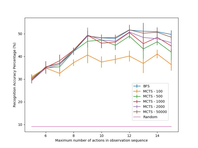
f (Harvest(U1 , R1 )) ! {Harvest(U1 , R1 )) : 1}
                                            f (Train(U2 , T )) !
                                                   {((HeavyRush)/{Attack(U3 , U4 )})\{Harvest(U1 , R1 )} : 1}
                                            f (Attack(U3 , U4 )) ! {Attack(U3 , U4 )) : 1}

                               ⇡ = [ Harvest(Worker 1 , Resource 1 ), Train(Barracks 1 , Heavy), Attack(Heavy 1 , Base 2 ) ]

        1)       Harvest(Worker 1 , Resource 1 )                     Train(Barracks 1 , Heavy)                     Attack(Heavy 1 , Base 2 )
        2) Harvest(U1 = Worker 1 , R1 = Resource 1 ) ((HeavyRush)/{Attack(U3 , U4 )})\{Harvest(U1 , R1 )} Attack(U3 = Heavy 1 , U4 = Base 2 )
                                                                                                          <
        3)                                                         (HeavyRush)/{Attack(U3 , U4 )}
                                                                                                                                               >
        4)                                                                   HeavyRush

                 Fig. 1. Sample CCG (top), example plan ⇡ (middle) and parse of three observed actions for a Heavy Rush (bottom)

plans, indicating where other actions are to be found relative                 tion and composition. The application combinator applies an
to an action. Those categories associated with the forward                     atomic category to a complex category of arity one while
slash operator are after the action, and those associated with                 composition combines two complex categories:
the backward slash are before it. In summary, categories are
                                                                                                 Rightward Application: X/Y               Y !X
functions that take other functions as arguments. We define
the root of some category G (atomic or complex) if it is the                                        Leftward Application: Y           X\Y ! X
leftmost atomic category in G. For example, for the complex                              Rightward Composition: X/Y                Y /Z ! X/Z
category ((C)\{A})\{B}, the root would be C.
                                                                               Intuitively, we can think of application and composition com-
   CCGs are defined by a plan lexicon, ⇤ = h⌃, C, f i, where ⌃
                                                                               binators as functional application and composition.
is a finite set of action types, C is a set of CCG categories (as
                                                                                  We now define a few terminology relevant to CCG-based
defined above), and f is a mapping function such that 8a 2 ⌃,
                                                                               plan recognition. We define ⇡ as a sequence of observed ac-
               f (a) ! {ci : p(ci |a), ..., cj : p(cj |a)}                     tions 1 , 2 , . . . k . Next, we define the CCG plan recognition
                                Pj                                             problem as PR = (⇡, ⇤, s0 ), where ⇡ is a subsequence of
where ci . . . cj 2 C and 8a k=i p(ck |a) = 1. This defini-                    observed actions, ⇤ is a CCG lexicon, and s0 is the initial
tion implies that action types can have multiple categories                    state of the world from where ⇡ was executed. The solution
associated with it in ⇤. Given a sequence of actions, these                    to the plan recognition problem is a pair (E, G), where G
probabilities represent the likelihood of assigning a category to              is a list of top-level goals that are being pursued in ⇡, and
an action for plan recognition. For details on these probabilities             E is a list of explanations or hypotheses that define the
and how they are used for plan recognition, see Geib [3].                      plan structures in ⇡. Figure 1 (bottom) shows the recognition
   We assume that all complex categories are leftward appli-                   of the observed sequence of actions ⇡ (Figure 1 (middle)),
cable (all arguments with the backward slash operator are                      which is a plan for the goal of executing a heavy rush in
discharged before any forward ones), and we only consider                      µRTS. First, a category is assigned to each action and its
complex categories with atomic categories for arguments.                       parameters bound based on the action (U1 = Worker 1 , R1 =
We also extend the definitions of action types and atomic                      Resource 1 , U3 = Heavy 1 , U4 = Base 2 ). This results in
categories to a first-order representation by introducing pa-                  the categories shown in line two of Figure 1. The cat-
rameters to represent domain objects and variables. CCGs with                  egory ((HeavyRush)/{Attack(U3 , U4 )})\{Harvest(U1 , R1 )}
parameterized actions and categories are defined by Geib [8].                  requires a Harvest(U1 , R1 ) to its left. Binding U1 to Worker 1
   Figure 1 provides an example CCG lexicon with parame-                       and R1 to Resource 1 unifies Harvest(U1 = Worker 1 , R1 =
terized action types and categories for recognizing a heavy                    Resource 1 ) with Harvest(U1 , R1 ) and allows leftward appli-
rush strategy in µRTS. Rush strategies consist of quickly                      cation to produce (HeavyRush)/{Attack(U3 , U4 )} shown in
constructing many units of a specific type, and having all those               line 3. This category expects a Attack(U3 , U4 ) to the right.
units attack the enemy. An example of a rush strategy from                     Rightward application can be used to produce HeavyRush.
the commercial RTS game Starcraft is Zerg rush. For this                       Since there are no more category arguments or actions, parsing
lexicon, ⌃ = {Harvest, Train, Attack} and C = {Harvest, At-                    ends with the hypothesis of the heavy rush plan, HeavyRush.
tack, ((HeavyRush)/{Attack})\{Harvest}}. The action types
Harvest(U1 , R1 ), Train(U2 , T ), and Attack(U3 , U4 ) each                                            III. R ELATED W ORK
have variable parameters representing different RTS units                         Monte-Carlo Tree Search (MCTS) is a well-known algo-
U1 , U2 , U3 , U4 , resource R1 , and unit type T . Since each                 rithm for game-playing and has been applied to both multi-
action type only has a single category, p(c|a) = 1.                            player [9], [10] and single player games [11]. For a survey
   In CCGs, combinators are operators defined over pairs of                    of MCTS algorithms in the literature, see Browne et al.
adjacent categories that are used to parse sequences of tokens.                [12]. Our work focuses on applying traditional MCTS for
The two most common types of combinators are applica-                          plan recognition for the domain of Real-Time Strategy (RTS)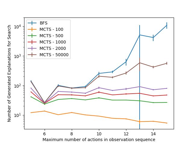
Games. Prior work applied bayesian programs to represent 1: procedure MCTS(⇡, ⇤, N, G)
2: T = root
plan knowledge for plan recognition in RTS games [13]. Our
3: for iter = 1 . . . N do
work focuses on representing plan knowledge using CCGs. 4: n = selection(T )
The problem of plan recognition can be viewed in many 5: if nE explains ⇡ then
different ways. Some approaches view the problem as a plan- 6: backpropagate(T, n, p(nE ))
ning problem (known as inverse-planning) [14]–[16]. Another 7: else
8: if nv = 0 then
way to view the problem is in the form of John McCarthy’s
9: reward = simulation(n)
circumscription [17]. Specifically, the seminal work by Kautz 10: backpropagate(T, n, reward )
and Allen [18] viewed plan recognition this way and repre- 11: else
sented plan knowledge in the form of a plan graph. 12: n0 = expansion(n)
Other plan recognition approaches view plan recognition as 13: if n0 = nil then
14: backpropagate(T, n0 , 0)
a form of parsing from Natural Language Processing using 15: else
a formal grammar that defines plan knowledge. To the best 16: reward = simulation(n0 )
of our knowledge, the first work to provide a correspondence 17: backpropagate(T, n0 , reward )
between the formal theory presented by Kautz and Allen [18] 18: end if
and Context-Free Grammars (CFGs) was Vilain [2]. This was 19: end if
20: end if
done by providing a mapping between plan graphs and CFGs. 21: end for
Since then, many other grammar formalisms have been used 22: end procedure
for plan recognition. Probabilistic State-Dependent Grammars,
an extension of Probabilistic Context-Free Grammar with state Fig. 2. MCTS CCG-based Plan Recognition
information, have also been used to represent plan knowledge
[19]. The plan recognition algorithm PHATT uses plan tree 1: procedure S ELECTION(T )
grammars [20] while YAPPR represents plan knowledge us- 2: n = Troot
3: N = nchildren
ing Plan Frontier Fragment Grammars [21], [22]. Our work 4: while N 6= ; do
focuses on using CCGs for plan recognition. 5: if n can have more children then
Plan recognition is tangentially related to goal recognition 6: return n
and has also been applied to games. One work applied Input- 7: else
Output Hidden Markov Models (IOHMM) to recognize player 8: s ⇠ U (0, 1)
9: if s > ✏ then
goals from low-level actions in a top-down action adventure 10: N 0 = argmax n0 2N n0r
game [23]. Other works have applied deep learning techniques 11: N 00 = argmax n0 2N 0 n0v
for goal recognition, such as stacked denoising autoencoders 12: return n0 ⇠ U (N 00 )
[24] and Long Short-Term Memory [25], [26]. 13: else
14: return n0 ⇠ U (N )
The work presented in this paper is closely related to the
15: end if
application of CCGs for plan recognition. The Breath-First 16: end if
Search (BFS) CCG-based plan recognition algorithm ELEXIR 17: end while
was first described by Geib [3]. ELEXIR has demonstrated 18: end procedure
a number of advantages over other work including efficient
recognition of partially-ordered plans and multiple interleaved Fig. 3. MCTS Selection Function
plans. This work was later extended to recognize plans with
loops [4].
Specifically, we employ Monte-Carlo Tree Search to recognize
sequences of observed actions.
IV. M ONTE -C ARLO T REE S EARCH A LGORITHM
Figure 2 provides high-level pseudocode of our CCG-based
The complexity of CCG-based plan recognition is defined Monte-Carlo Tree Search (MCTS) plan recognition algorithm.
by the number of categories per action type in a CCG lexicon, The MCTS algorithm takes as input a sequence of observed
and the number of actions in an observed action sequence. As actions ⇡ = h 1 , ..., k i, a CCG lexicon ⇤, the maximum
the number of categories per action increases, the branching number of iterations for search N , and a set of query goals
factor from search increases. Coupled with a large number G (goals that we want to recognize). We will describe how to
of actions in an observed action sequence, the search space compute p(g|⇡) (g 2 G) after describing the MCTS algorithm.
for plan recognition can significantly increase. As a result, In our description of the MCTS approach, we use U to refer
Breath-First Search (BFS) plan recognition does not scale well to a uniform distribution and x ⇠ U (X) or k ⇠ U (i, j) as
for large CCG lexicons. Prior CCG learning algorithms like sampling from a set X from the interval [i . . . j].
LexGreedy were successfully able to scale learning to long Our algorithm starts by initializing a search tree T with a
plans. However, the learned CCG lexicons were too large for single root node. Each node in the search tree is defined as
BFS plan recognition. Our solution is the development of an n = hE, ci , r, vi, where E is an explanation of 1 . . . i 2 ⇡
anytime approximation algorithm plan recognition algorithm. (where i is the depth of the node and 1 i k), ci is the
f (Harvest(U1 , R1 )) ! {Harvest(U1 , R1 )) : 0.5,
                                                                              (Harvest(U1 , R1 ))/{Harvest(U2 , R2 )} : 0.5}
                                                                           f (Train(U2 , T )) !
                                                                              {((HeavyRush)/{Attack(U3 , U4 )})\{Harvest(U1 , R1 )} : 1}
                                                                           f (Attack(U3 , U4 )) ! {Attack(U3 , U4 )) : 1}

                             (a) Example Execution                                                (b) CCG Lexicon
                                       Fig. 4. Example of MCTS Execution (Left) with CCG (Right)

 1: procedure S IMULATION(n)                                         Our approach uses ✏-greedy as the tree policy. Algorithm 3
 2:    Let E = nE (explanation in n for    1   ...   i)
                                                                     provides pseudocode for the selection function. We refer to
 3:    for l 2 i+1 . . . k do
 4:       Let a be the action type of l                              nchildren as the set of node n’s children. First, the function
 5:       C = valid (⇤f (a) )                                        checks to see if the current node n can have more children
 6:       c ⇠ U (C)                                                  (lines 5-6 of Figure 3). If all children nodes have been
 7:       E 0 = extend (E, c)                                        constructed for n, then the ✏-greedy policy selects the next
 8:       E ⇠ U (E 0 )                                               node based on the highest reward and times visited (lines 8-
 9:    end for
                                                                     15 of Figure 3).
10: end procedure
                                                                        If the selected node n (line 4 of Figure 2) has an explanation
                Fig. 5. MCTS Simulation Function                     nE for ⇡ (i.e. node is a leaf), there is no need to expand
                                                                     that node and thus, MCTS back-propagates the reward p(nE )
                                                                     (line 4-5 of Figure 2). This reward is the probability of the
category assigned to an observed action i , r is the reward,         explanation nE , and will be explained below.
and v is the number of times the node was visited. The root             Second, expansion constructs successor nodes N given
node (depth 0) is initialized to root = hnil , nil , , 0i.           the selected node n = hE, ci 1 , r, vi from the selection
   Each edge in the search tree represents the extension of an       function. Intuitively, expansion extends the explanation nE for
explanation E. Explanations define plan structures found in the        1 . . . i 1 given the next observed action i and one of its
observed actions ⇡ and are represented as a list of atomic or        mapped categories in the lexicon ⇤. First, expansion gets a list
complex categories. An explanation with multiple categories          of valid categories C (categories whose leftward arguments
means that the agent is pursuing multiple, potentially inter-        can be parsed) for an observed action i 2 ⇡. Expansion
leaved plans. Atomic categories in explanations define top-          then selects a category c0i 2 C with a uniform weighted
level plans that the agent is pursuing while complex categories      distribution based on the category’s conditional probabilities
mean that one of the plans in ⇡ is incomplete, and more actions      p(c0i |a), where a is the action type of i . Next, expansion
are needed to complete that plan. The extension method for           extends the current explanation E with c0i , resulting in a set of
an explanation used by MCTS is similar to the one used by            explanations E 0 . For each explanation e 2 E 0 , the expansion
the ELEXIR plan recognition algorithm [3]. An explanation            function constructs a new node n0 = he, c0i , , 0i and adds it
E for 1 . . . i 1 is extended by assigning a category c to           to the set of n’s children. The last constructed node is then
an observed action i 2 ⇡, and adding it to E. Next, known            returned for simulation.
CCG combinators (defined in Section II) are used to parse               We note that nodes not returned for simulation will not
these categories which results in a new explanation (list of         be part of the search tree until later. These nodes will have
potentially new atomic or complex categories). See Figure 4a         their times visited set to 0 until they have the opportunity to
for an example of a few explanations (explanations are closed        be placed into the search tree when the ✏-greedy tree policy
in brackets “[” and “]”).                                            selects them during selection (line 14 of Figure 3). If the
   Our approach follows the standard approach to MCTS:               selection function chooses one of these nodes, then MCTS
selection, expansion, simulation, and back-propagation. We           directly simulates and back-propagates from the node as it was
look at each function in detail. First, selection chooses the        already constructed during expansion (lines 8-10 in Figure 2).
next node in the search tree to expand using a tree policy.          If there are no valid categories or no explanations are generated
by extending E with c0i , then expansion fails (returns nil) and To this end, we run two different experiments to test the
a reward of 0 is back-propagated (lines 13-14 of Algorithm 2). effectiveness of MCTS plan recognition. First, we analyze the
Third, simulation “plays” out plan recognition from node performance of MCTS to understand how well MCTS can
n0 = hE, c0i , , 0i using a random playout policy. We chose successfully recognize sequences of observed actions. Second,
a random playout policy because it worked well in our we analyze the scalability of the search tree against observation
experiments. Figure 5 provides pseudocode for the simulation length. For each experiment, we compare against a Breath-
function. Given an observed action l 2 i+1 . . . k (where k First Search (BFS) plan recognition algorithm in ELEXIR [3].
is the index of the last observed action, and i + 1 l k), Both approaches are evaluated on the µRTS domain. µRTS is a
simulation first retrieves a list of valid categories C for i+1 minimalistic RTS game designed to evaluate AI research in an
from the set of all mapped categories ⇤f (a) , where a is the RTS setting [27]. Compared to commercial RTS games such as
action type of i+1 , and samples a category c 2 C uniformly at StarCraft, µRTS maintains those properties of RTS games that
random (lines 4-6). Next, simulation extends E 0 with c, gets a make them complex from an AI point of view (i.e. durative
list of new explanations, and samples an explanation uniformly and simultaneous actions, real-time combat, large branching
at random (lines 7-8). Once the simulation successfully plays factors, and full or partial observability). This work focuses on
out plan recognition, a numerical reward, computed as the recognizing strategies in deterministic, fully observable games.
probability of the explanation at the leaf node p(E), is All CCGs are constructed using the CCG learning algorithm
returned. This probability is computed in the same manner Lex Greedy [6]. Lex Greedy requires an initial CCG lexicon
as that described by Geib [3]. Intuitively, this probability ⇤init , and a training dataset consisting of sequences of actions
represents how well the explanation describes the observed (called plan traces). We use a collection of scripted game
actions ⇡. A higher probability explanation means that this agents to generate learning datasets and ⇤init . The process
is a more likely description of the plans being executed in is described below.
⇡. Finally, back-propagation updates the statistics (reward r Plan traces are constructed using replay data from gameplay
and number of times visited v) along the path from n to of the scripted agents. A replay is a trace of a game represented
the root. For each ancestor n = hE, ci , r, vi on the path, as a sequence of state, player action tuples containing the
back-propagation updates r and normalizes the result, and evolution of the game state as well as the actions performed
increments v. by each player during the game. We construct a replay
Plan recognition entails finding a set of the most probable dataset was created by running a 5-iteration round-robin
top-level goals being pursued G 2 G and a set of explanations tournament using the following built-in scripted agents: PO-
E for an observation sequence ⇡. In this work, we assume ⇡ LightRush, POHeavyRush, PORangedRush, POWorkerRush,
is pursuing a single goal g (i.e. |G| = 1). The result of MCTS EconomyMilitaryRush, EconomyRush, HeavyDefense, Light-
is a tree T where the leaves are explanations for ⇡. Thus, Defense, RangedDefense, WorkerDefense, WorkerRushPlus-
E is defined as the leaves of T . Given E, we can compute Plus. Each agent played against each other as both player
p(g|⇡) (conditional probability that ⇡ is pursuing g) in the 1 and player 2 on the open maps of the CIG 2018 µRTS
same manner as ELEXIR [3], tournament.2 We chose these agents over other agents such
P as NaiveMCTS because they execute a defined strategy which
e2E p(e)
p(g|⇡) = P g we could use as the goal for learning and plan recognition.
e2E p(e) We then generated a learning dataset of plan traces with their
where Eg is the set of explanations where g is the root of at corresponding goals using the replay dataset. For each replay
least one of the categories in the explanation. in the replay dataset, we generated two plan trace/goal pairs:
Figure 4a provides the execution of a single iteration of one for each agent in the replay. Each pair was constructed by
MCTS given the CCG lexicon in Figure 4b and the se- parsing player actions done by an agent, and using the agent
quence of observed actions ⇡ from Figure 1. For simplic- itself as the goal (i.e., the goal of plan recognition will be to
ity, we provide these actions as blue circles in Figure 4a identify which of the agents does a plan trace come from).
(first action is the top circle). First, the selection function Lex Greedy has two tunable parameters: abstraction thresh-
chooses a node in the tree without children (red box): old and pruning threshold ⌧ . controls the hierarchical
n = h[Harvest(U1 , R1 )], Harvest(U1 , R1 ), 1.0, 1i. Second, the structures constructed during learning, and is defined by a per-
expansion function constructs a new node n0 by extending centage of the training dataset. The pruning threshold removes
explanation nE = [Harvest(U1 , R1 )] (green box). Third, sim- categories from the lexicon whose conditional probability
ulation plays out plan recognition to get an explanation for ⇡ p(c|a) (a is an action type, c is a category) that are below
(purple hexagon): [HeavyRush], r = 1.0. Finally, the reward ⌧ . For our experiments, we set = 50% and ⌧ = 0 (which
of 1 is back-propagated through the ancestor nodes (nr = indicates no pruning of the CCG lexicon). Our MCTS plan
2.0, n0r = 1.0, root r = 0.66, and nv = 2, n0v = 1, root v = 3). recognition approach also has two tunable parameters: number
of iterations N and ✏-greedy threshold ✏. For our experiments,
V. E XPERIMENTAL E VALUATION we set N = 100, 500, 1000, 2000, 50000, and ✏ = 0.4.
The purpose of MCTS plan recognition is to scale search
to large CCG lexicons while maintaining good performance. 2 https://sites.google.com/site/micrortsaicompetition/rulesnumber of categories per action type did not deviate from the
average by a significant amount over the 5 runs.
Figure 7a provides average recognition accuracy for ob-
servation sequences with a maximum of 5 to 15 actions
(higher is better). Overall, we see an expected trend for all
iterations of MCTS and BFS. As the number of iterations
for MCTS increases, the goal prediction accuracy increases.
We also see that, as we increase the number of iterations,
MCTS converges to the performance of BFS. This is because
predicting a goal for BFS and MCTS relies on the set of
generated explanations, and the set of explanations constructed
by MCTS is a subset of the explanations constructed by BFS.
Fig. 6. Average Number of Categories For Action Types Thus, BFS provides an upper bound on the performance of
CCG-based plan recognition. Furthermore, both MCTS and
We evaluate MCTS and BFS using four metrics: average BFS outperformed a random predictor. We define a random
goal prediction accuracy, average percentage of actions seen predictor as one that chooses a goal at random to recognize
before recognition, average number of explanations generated an observation sequence. Since we have 11 possible goals, a
for plan recognition, and average recognition execution time. random predictor would have an average accuracy of 9.09%.
We compute goal prediction accuracy as follows: We also see that lower number of actions in an observation
sequence requires less iterations of MCTS to converge to BFS.
Number of correctly predicted goals For example, for observation sequence lengths of 5-8 actions,
Accuracy = 100 ⇤
Total number of instances we see that we only need 500 iterations of MCTS to converge.
The percentage of actions before recognition is computed as On the contrary, as the number of actions in the observation
the minimum number of actions in an observation sequence sequence increases, we see that complete convergence requires
required before a plan recognition algorithm predicts the more iterations. In Figure 7a, we see that 50000 iterations of
goal, and continues to predict that goal until the end of the MCTS was not enough to completely converge to BFS. Given
observation sequence. The explanations generated for plan this trend, we can see that longer observation sequences will
recognition are those that explain the observed sequence of require more iterations of MCTS.
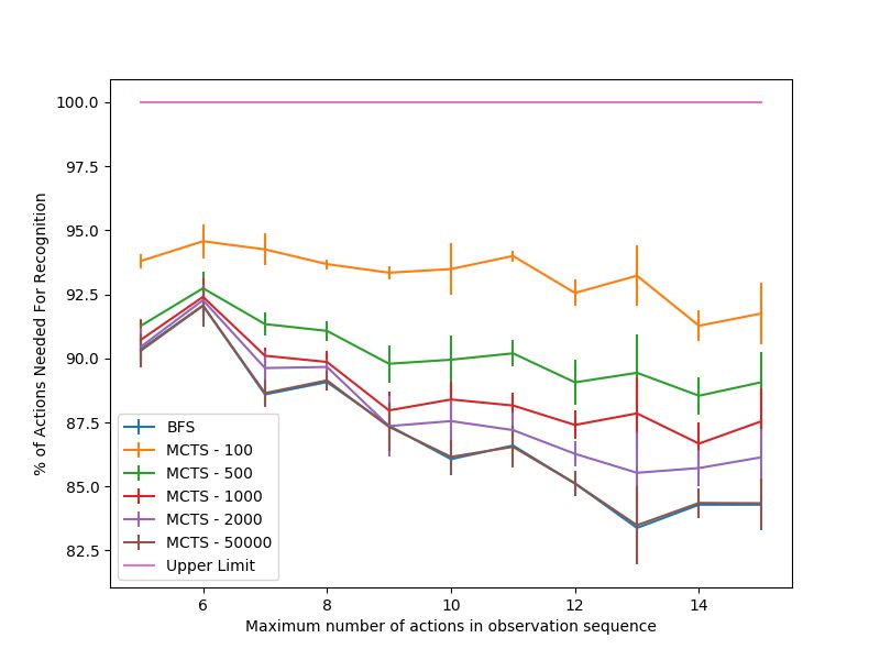
actions given to the plan recognition algorithm. As such, to Figure 7b provides the average percentage of actions re-
compute the number of explanations, we count the number of quired to recognize the goal of an observation sequence
leaves in the search tree. Finally, recognition execution time (lower is better). Similar to that of prediction accuracy, MCTS
is the number of seconds that a plan recognition algorithm converges to the performance of BFS as the number of
executed. We gather these metrics for observations sequences iterations increases. We see that by 50000 iterations, MCTS
with a maximum of 5 to 15 actions. All metrics are averaged successfully converges to BFS. Additionally, we also see that
over all testing instances, and then averaged over 5 runs. To MCTS and BFS do not require all actions in the observation
provide additional insight for each metric, we also compute the sequence to recognition a plan (denoted by Upper Limit
standard deviation over the 5 runs. For each run, we randomly in Figure 7b). However, unlike prediction accuracy, lower
shuffled all instances in the learning dataset, and split the iterations of MCTS do not converge at shorter observation
dataset into 80% training and 20% testing. sequence lengths. This is most likely because this metric
Figure 6 plots the number of categories for action types depends on the structure of the complex categories in the
in the learned CCG lexicon against the maximum number of lexicon. Categories with more leftward arguments will delay
actions in the observation sequence. All learned CCG lexicon recognition of a goal to later in the plan while those with more
contain 465 action types, each corresponding to player actions rightward arguments will allow for earlier recognition.
done in game by the scripted agents. We see that the minimum Figure 8a plots the average number of explanations gen-
number of categories for an action type is 1. This is because erated for plan recognition against the maximum number of
one of the requirements for Lex Greedy is that all action types actions in an observation sequence (graphed using logarithmic
in the learned CCG must have at least one category associated scale). Overall, we see that MCTS successfully scales the
with it. We also see that the maximum number of categories for number of generated explanations. Furthermore, we also see
an action type is rather high, even going up to 100 categories that as the number of iterations of MCTS increases, the
for a single action type. However, we note that the average number of explanations generated also increases and converges
number of categories per action type is quite low. This implies to BFS. Recall that the number of explanations generated
that our learned CCGs are sparse in that many of the action by MCTS is a subset of the explanations of BFS. Thus,
types in the CCG are not associated with learned categories. given an infinite number of iterations, MCTS should converge
However, as we will see, this does not reduce the complexity to BFS. An interesting observation is that MCTS still has
of plan recognition. Another interesting point is that, the good performance despite generating less explanations than
maximum number of categories for an action type and the BFS. In Figure 7a, 500 iterations of MCTS converged to the(a) Average Prediction Accuracy (higher is better) (b) Average Percentage of Actions Before Recognition
of Goal (lower is better)
Fig. 7. Average of Performance Metrics for MCTS and BFS
(a) Number of Explanations after Plan Recognition (b) Recognition Time (seconds)
Fig. 8. Average of Scaling Metrics for BFS and MCTS (lower is better)
performance of BFS given observation sequences with 5-8 of explanations and therefore took longer to execute). Looking
actions. However, as seen in Figure 8a, MCTS only generated closely at our data, we noticed that, for one of the runs,
a fraction of the explanations of BFS. Thus, we believe some BFS generated millions of explanations for one observation
explanations are ignored by MCTS as they may not be needed sequence, and took approximately 448 seconds to execute.
to recognize the goal. We also see a steep reduction in the Similarly, for MCTS with 50000 iterations, one observation
number of explanations for 6 action observation sequences. sequence took approximately 386 seconds. However, looking
This is due to the complex categories in the generated lexicon at the median number of explanation and recognition time,
for that length being more leftward than rightward, which we see significantly lower values (359 explanations and 0.72
reduces the number of generated explanations [3]. This aligns seconds for BFS, and 3.55 seconds for MCTS with 50000
with Figure 7b, where both BFS and MCTS needed to see iterations) than the mean. This confirms that there are outlier
more actions in the plan prior to recognition. observation sequences that required more time and number
Figure 8b provides the average amount of time (in sec- of explanations than other sequences. These outliers are still
onds) for plan recognition to complete. Overall, we see that important. In Real-Time Strategy games, long recognition time
MCTS scales significantly better than BFS after observation for even a single observation sequence could prove costly as it
sequences with 13 actions. We also observe that recognition could be the difference between victory and defeat in a game.
time is lower for lower number of MCTS iterations. Figure 8b For observation sequences with a maximum of 13 actions,
also shows that the recognition time for MCTS mostly does BFS failed to recognize several of the testing instances because
not vary significantly from the average. it ran out of memory for one of the runs. To understand why
Both BFS and MCTS with 50000 iterations has a very large this happened, we looked the learned CCG lexicon that was
standard deviation in recognition time, and BFS had a large constructed for that run and the observation sequences that
deviation for the number of explanations for observation se- failed. We noticed that one action in particular was repeated
quences of 13 actions. We believe this is due to outliers in the in the sequence: the action for constructing a worker unit. This
data (observation sequences which generated a large number action was repeated 6, 7, and even 11 times, which is 85% ofthe observation sequence. In the CCG lexicon, this action type [10] D. Silver, J. Schrittwieser, K. Simonyan, I. Antonoglou, A. Huang,
contained 23 categories. Assuming all categories are viable A. Guez, T. Hubert, L. Baker, M. Lai, A. Bolton, Y. Chen, T. Lillicrap,
F. Hui, L. Sifre, G. van den Driessche, T. Graepel, and D. Hassabis,
and can be assigned to each action in the sequence (all leftward “Mastering the game of Go without human knowledge,” Nature, vol.
arguments for the categories can be discharged), the number 550, no. 7676, p. 354, 2017.
of possible explanations would explode the search space (for [11] M. P. D. Schadd, M. H. M. Winands, H. J. Van Den Herik, G. M.-
B. Chaslot, and J. W. H. M. Uiterwijk, “Single-player monte-carlo
11 repetitions of the action, we can have 1123 explanations). tree search,” in International Conference on Computers and Games.
Thus, even if the observation sequence length is not very high, Springer, 2008, pp. 1–12.
BFS can exhaust all memory for search if the branching factor [12] C. B. Browne, E. Powley, D. Whitehouse, S. M. Lucas, P. I. Cowling,
P. Rohlfshagen, S. Tavener, D. Perez, S. Samothrakis, and S. Colton, “A
is high. However, MCTS did not exhaust all memory for these survey of monte carlo tree search methods,” Computational Intelligence
observation sequences. This demonstrates the effectiveness of and AI in Games, IEEE Transactions on, vol. 4, no. 1, pp. 1–43, 2012.
MCTS in reducing the search space for plan recognition. [13] G. Synnaeve and P. Bessiere, “A Bayesian Model for Plan Recognition in
RTS Games Applied to StarCraft,” in Proceedings of 7th AAAI Artifical
Intelligence Interactive Digital Entertainment Conference, 2011, pp. 79–
VI. C ONCLUSION 84.
[14] M. Ramirez, H. Geffner, M. Ram, and H. Geffner, “Probabilistic Plan
This paper described a Monte-Carlo Tree Search (MCTS) Recognition Using Off-the-Shelf Classical Planners,” in Proceedings of
CCG-based plan recognition algorithm. Specifically, we em- the 24th AAAI Conference on Artificial Intelligence, 2010, pp. 1121–
ployed traditional MCTS to find a set of explanations and 1126.
[15] M. Ramı́rez and H. Geffner, “Goal recognition over POMDPs: Inferring
predict the goal of a given sequence of observed actions. We the intention of a POMDP agent,” in Proceedings of the 22nd Interna-
demonstrated that traditional MCTS was successful in scaling tional Joint Conference on Artificial Intelligence, 2011, pp. 2009–2014.
for large CCG lexicons while maintaining good performance [16] D. Höller, G. Behnke, P. Bercher, and S. Biundo, “Plan and goal recog-
nition as HTN planning,” in 2018 IEEE 30th International Conference
(below that of exhaustive search, but significantly better than on Tools with Artificial Intelligence. IEEE, 2018, pp. 466–473.
a random prediction baseline). We saw that MCTS was able [17] J. McCarthy, “Circumscription—a form of non-monotonic reasoning,”
to significantly reduce the number of explanations generated Artificial Intelligence, vol. 13, no. 1-2, pp. 27–39, 1980.
[18] H. A. Kautz and J. F. Allen, “Generalized Plan Recognition,” in
during plan recognition compared to BFS. For future work, Proceedings of the 5th AAAI Conference on Artificial Intelligence,
we would like to improve our MCTS algorithm by looking ser. AAAI’86. AAAI Press, 1986, pp. 32–37. [Online]. Available:
into different optimizations made for MCTS in the literature. http://dl.acm.org/citation.cfm?id=2887770.2887776
[19] D. V. Pynadath and M. P. Wellman, “Probabilistic state-dependent
We also would like to look into potentially augmenting MCTS grammars for plan recognition,” in Proceedings of the 16th Uncertainty
with machine learning techniques, as they has been shown to in Artificial Intelligence, 2000, pp. 507–514. [Online]. Available:
be successful recently in other game playing domains [10]. http://dl.acm.org/citation.cfm?id=2074005
[20] C. W. Geib and R. P. Goldman, “A probabilistic plan recognition
Finally, we want to look into applying MCTS for the problem algorithm based on plan tree grammars,” Artificial Intelligence, vol. 173,
of CCG-based planning. no. 11, pp. 1101–1132, 2009.
[21] C. W. Geib, J. Maraist, and R. P. Goldman, “A new probabilistic
R EFERENCES plan recognition algorithm based on string rewriting,” in Proceedings
of the 18th International Conference on Automated Planning
[1] C. F. Schmidt, N. S. Sridharan, and J. L. Goodson, “The plan recognition and Scheduling, 2008, pp. 91–98. [Online]. Available: http:
problem: An intersection of psychology and artificial intelligence,” //www.aaai.org/Papers/ICAPS/2008/ICAPS08-012.pdf{%}5Cnpapers2:
Artificial Intelligence, vol. 11, no. 1-2, pp. 45–83, 1978. //publication/uuid/BF162044-C60C-4B71-864C-F70C78A39274
[2] M. Vilain, “Getting Serious About Parsing Plans: A Grammatical [22] C. W. Geib and R. P. Goldman, “Handling Looping and
Analysis of Plan Recognition.” in Proceedings of the 8th AAAI Optional Actions in YAPPR,” in Proceedings of the 5th AAAI
Conference on Artificial Intelligence, 1990, pp. 190–197. [Online]. Conference on Plan, Activity, and Intent Recognition, 2010,
Available: http://www.aaai.org/Papers/AAAI/1990/AAAI90-029.pdf pp. 17–22. [Online]. Available: http://www.aaai.org/ocs/index.php/
[3] C. W. Geib, “Delaying commitment in plan recognition using combi- WS/AAAIW10/paper/viewPDFInterstitial/2001/2442{%}5Cnpapers2:
natory categorial grammars,” in Proceedings of the 21st International //publication/uuid/BCCB6A23-7F82-4470-AEF6-19EFE298CA11
Joint Conference on Artificial Intelligence, 2009, pp. 1702–1707. [23] K. Gold, “Training Goal Recognition Online from Low-Level Inputs in
[4] C. W. Geib and R. P. Goldman, “Recognizing plans with loops an Action-Adventure Game,” in Proceedings of the 6th AAAI Conference
represented in a lexicalized grammar,” in Proceedings of the 25th on Artificial Intelligence and Interactive Digital Entertainment, 2010,
AAAI Conference on Artificial Intelligence, 2011, pp. 958–963. pp. 21–26.
[Online]. Available: http://www.aaai.org/ocs/index.php/AAAI/AAAI11/ [24] P. Vincent, H. Larochelle, I. Lajoie, Y. Bengio, and P.-A. Manzagol,
paper/viewFile/3698/3985 “Stacked denoising autoencoders: Learning useful representations in a
[5] C. W. Geib and P. Kantharaju, “Learning Combinatory Categorial deep network with a local denoising criterion,” Journal of Machine
Grammars for Plan Recognition,” in Proceedings of the 32nd AAAI Learning Research, vol. 11, pp. 3371–3408, 2010.
Conference on Artificial Intelligence, 2018. [25] W. Min, E. Y. Ha, J. P. Rowe, B. W. Mott, and J. C. Lester, “Deep
[6] P. Kantharaju, S. Ontañón, and C. W. Geib, “Extracting CCGs for Learning-Based Goal Recognition in Open-Ended Digital Games.” Pro-
plan recognition in RTS games,” in In Proceedings of the Workshop ceedings of the 10th AAAI Conference on Artificial Intelligence and
on Knowledge Extraction in Games 2019, 2019. Interactive Digital Entertainment, pp. 37–43, 2014.
[7] H. Curry, Foundations of Mathematical Logic. Dover Publications Inc., [26] W. Min, B. W. Mott, J. P. Rowe, B. Liu, and J. C. Lester, “Player
1977. Goal Recognition in Open-World Digital Games with Long Short-Term
[8] C. W. Geib, “Lexicalized Reasoning About Actions,” Advances in Memory Networks.” in Proceedings of the 25th International Joint
Cognitive Systems, vol. Volume 4, pp. 187–206, 2016. Conference on Artificial Intelligence, 2016, pp. 2590–2596.
[9] D. Silver, A. Huang, C. J. Maddison, A. Guez, L. Sifre, G. Van Den [27] S. Ontañón, “The combinatorial multi-armed bandit problem and its
Driessche, J. Schrittwieser, I. Antonoglou, V. Panneershelvam, M. Lanc- application to real-time strategy games,” in Proceedings of the 9th AAAI
tot, S. Dieleman, D. Grewe, J. Nham, N. Kalchbrenner, I. Sutskever, Conference on Artificial Intelligence and Interactive Digital Entertain-
T. Lillicrap, K. Kavukcuoglu, M. Leach, T. Graepel, and D. Hassabis, ment, 2013, pp. 58–64.
“Mastering the game of Go with deep neural networks and tree search,”
Nature, vol. 529, no. 7587, p. 484, 2016.You can also read