Shift of the storm surge season in Europe due to climate variability
←
→
Page content transcription
If your browser does not render page correctly, please read the page content below
www.nature.com/scientificreports
OPEN Shift of the storm surge season
in Europe due to climate variability
Jean‑Baptiste Roustan1,2*, Lucia Pineau‑Guillou1, Bertrand Chapron1, Nicolas Raillard3 &
Markus Reinert4
Along the European coasts, changes in the timing of the storm surge season are analyzed. Using 10
long-term tide gauges located in western Europe, a consistent spatio-temporal shift emerged in the
storm surge season between 1950 and 2000. Temporal shifts are positive (later events) in the North,
negative (earlier events) in the South. Extreme surge events occurred about 4 days/decade later in
northern Europe, and 5 days/decade earlier in southern Europe. Such a tendency is similar to the one
already reported for European river floods between 1960 and 2010. In northern Europe, extreme
surges are known to occur during the positive North Atlantic Oscillation phase (NAO+). Identified
spatio-temporal shifts likely trace that NAO+ storms tend to occur later between 1950 and 2000. A
new index measuring the timing of the NAO+ and NAO− persistent situations is shown to help capture
this spatial distribution in the timing of the storm surge seasons.
In the North-East Atlantic, storm surges are fingerprints of extra-tropical storms. As they depend on storm
trajectories, storm surge amplitudes greatly depend on the site location. They are larger in northern Europe,
with values reaching 3 m in the North Sea, but surges are usually not more than 1 m in southern Europe along
the Spanish and Portuguese coasts1. The North Sea 1953 flood, with up to 3.3 m measured surge, was one of the
most devastating natural disasters in western Europe last century, with more than 2000 reported deaths in the
Netherlands and in southeast England2,3. More recently, Xynthia storm hit the French coasts in February 2010,
generating a major fl ooding4 with 47 deaths and around 10 000 people had to be e vacuated5. The storm surge
reached 1.5 m at La Rochelle harbour, the highest level ever observed since the tide gauge installation in 1 9976.
Combining tide gauge record and historical information, such a value was estimated to occur less than once
every 100 years7.
The influence of climate change on extra-tropical storms, their frequencies, intensities and trajectories, is thus
the subject of a large number of studies. In a warming climate, a possible expansion of the Hadley cell would lead
the jet streams and storm tracks to move poleward8. Changes in mid-latitudes storm tracks have been reported
since the 1980s9. Importantly, any change in the frequency, tracks, displacement speed or intensity of storms
will then also be traced in the observed storm surge. Many authors thus investigated the variability and trends in
storm surges over the last century at quasi-global s cale1,10,11, at regional scale, e.g. in the English c hannel12, along
the European c oasts13, in southern E urope14, along the U.S. c oasts15,16, in the western North Pacific17, or at local
scale, e.g. at New York18. At first order, changes in storm surges are relative to changes in mean sea level1,19. After
removing the mean sea level contribution, storm surges display strong interannual to multidecadal variability,
and this variability is mainly controlled by the large-scale atmospheric forcing. Indeed, high correlations between
storm surges and climate indices are found1,11,16. Still, there is no clear long-term (i.e. centennial) trend in storm
surges11–13, even though trends can be detected on shorter periods. In their review, Feser et al.20 concluded that
the trends in storm activity critically depend on the analyzed time period. In the North Atlantic, over the last
decades, the number of storms tend to increase north of about 55 N (and decrease southward), but consider-
ing more than 100 years, there is large decadal variations, and either no trend or a decrease in storm numbers.
While all these studies focus on changes in the intensity and frequency of storm surges, very few studies focus
on possible changes in the timing of storm surges. In the North-East Atlantic, storm surges show an expected
strong annual cycle. Storm surges more likely occur between December and January10. More precisely, at Brest
(France), Reinert et al.21 reported a clear shift in the storm surge timing. From the analysis of more than 150 years
of tide gauge data, extreme events were found to occur three weeks earlier (mid-December instead of beginning of
January) in the winter 2000 than in the 1950s. Analysis of additional nearby stations suggests a large-scale process.
1
IFREMER, Laboratoire d’Océanographie Physique et Spatiale, UMR 6523 (IFREMER, CNRS, IRD, UBO),
IUEM, Brest, France. 2Direction Générale de l’Armement, Ministère des armées, Paris, France. 3IFREMER,
RDT, Brest, France. 4Leibniz Institute for Baltic Sea Research Warnemünde, Rostock, Germany. *email:
jean-baptiste.roustan@polytechnique.edu
Scientific Reports | (2022) 12:8210 | https://doi.org/10.1038/s41598-022-12356-5 1
Vol.:(0123456789)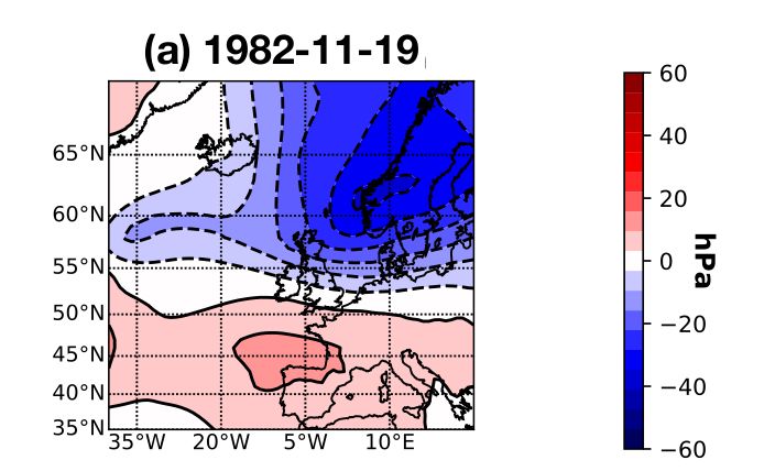
www.nature.com/scientificreports/
~
Figure 1. Location of the tide gauge stations from the GESLA-2 database. Labelled stations are the ones used in
this study.
The first objective of this paper is to expand on this result and to investigate whether the shift of the storm
surge season, revealed at Brest, is also a large-scale spatio-temporal process, distributed along the European
coasts. The second objective is to investigate the role of the large-scale climate variability on such a shift.
The paper is organised as follows. The first section describes the ocean and atmospheric data used in our
study. The next section describes the two different methods used to compute the timing of the storm surge season,
the first one being parametric, the second being non-parametric. Then, we present the results: the large-scale
shift observed in the storm surge season between 1950 and 2000, and the link with the North Atlantic climate
variability. Finally, we discuss a possible shift in the timing of the storms in the North Atlantic, revealed by the
analysis of a new climate persistence index.
Data
Sea level data. We used the global sea level dataset GESLA-2 (Global Extreme Sea Level Analysis Version
2)22. This dataset, released in 2016, provides high-frequency (i.e. hourly or subhourly) sea level records from tide
gauges at as many locations worldwide as possible, i.e. 1355 stations. Data were assembled from 30 providers, the
most important being UHSLC (University of Hawaii Sea Level Center)23. In GESLA-2 global dataset, the average
record length is 29 years, and the maximum length is 167 years in the case of Brest, France.
In addition to sea level records, GESLA-2 provides the surges at each s tation1. These surges, used in our study,
are skew surges (and not instantaneous surges), defined as the difference between the maximum observed sea
level and the maximum tide prediction during a tidal c ycle24. The last 15 years were used to compute the tidal
constituents, including the annual and semi-annual signals1. Note that the tide used to compute the skew surge
does not include Mean Sea Level (MSL), so any variation in the MSL, such as MSL r ise25,26 or interannual vari-
ability, remains in the surge data. This concern will be addressed later, adding a linear trend in the parameter
formulation (see Eqs 2 and 3).
We selected stations along the North-East Atlantic coasts with at least 50 years of data, to investigate a pos-
sible shift between the 1950s and the year 2000. Note that a year is considered as complete, when it contains
more than 300 days of data (82% complete). This led to selecting 10 stations (Fig. 1). Half of them are located in
the North-East Atlantic (Vigo, La Coruña, Santander, Brest and Newlyn), and the other half in the North Sea
(Dover, Immingham, Cuxhaven, Esbjerg and Tregde). The time spans for each station are displayed in Table S1
(Supplementary).
Atmospheric data. To investigate the role of the North Atlantic atmospheric circulation: (1) we used NAO
(North Atlantic Oscillation) data, (2) we considered atmospheric data from a weather reanalysis, and (3) we
defined and computed a new index, the NAOP (NAO Persistence) timing index.
(1) The NAO refers to the main mode of variability of the atmosphere in the North A tlantic27,28. This index
corresponds to the difference of Sea Level Pressure (SLP) between the Azores high pressure and Iceland
low pressure systems, averaged over long periods (e.g. monthly, seasonal, annual). We used the wintertime
(December to March) Hurrell station-based NAO Index (retrieved from https://c limat edata guide.u car.e du/
climat e-d
ata/h
urrel l-n
orth-a tlant ic-o
scill ation-n
ao-i ndex-s tatio
n-b
ased, last access: April 2020). This index
is computed as the difference of normalized average winter SLP between Lisbon (Portugal) and Stykkishól-
mur/Reykjavik (Iceland), over the period 1864–2019. In addition to this ‘winter’ NAO index, we computed
similarly a ‘daily’ NAO index, based on SLP data from atmospheric reanalysis—see below point (2).
Scientific Reports | (2022) 12:8210 | https://doi.org/10.1038/s41598-022-12356-5 2
Vol:.(1234567890)www.nature.com/scientificreports/
(2) We used SLP and 10-meter winds from Twentieth Century Reanalysis version 3 (20CR)29,30, a historic
weather reconstruction from 1836 to 2015, with a 1° gridded global coverage. The temporal resolution is
3 hours for SLP and winds. We used these data to detect if there is any seasonal shift in the atmospheric
data, but also to compute a ‘daily’ NAO index. To do so, we have first checked that the ‘winter’ NAO index
computed from 20CR was very close to the Hurrell station-based winter NAO index, over the period
1900–2014. A correlation coefficient of 0.98 between these two indices confirms that 20CR well reproduces
NAO climate indices. We then computed a ‘daily’ NAO index similarly to the ‘winter’ NAO index, except
that the 20CR SLP data were averaged every day (instead of every winter). This ‘daily’ NAO index will be
used further to compute a new index (see below). Note that we used 20CR data only over the 20th century,
where we checked that the reanalysis correctly tracks the NAO index.
(3) We defined a new index: the NAOP (NAO Persistence) timing index. This NAOP+ (NAOP−) timing
index corresponds to the period of the winter, where the persistence in a NAO+ (NAO−) regime is maxi-
mum (Fig. 6a and c). It is computed every winter (December–February) as the median date of the longest
period with the ‘daily’ NAO over (under) a threshold. Here, the threshold is 2.5 and the daily NAO index
is computed from 20CR SLP data (see above). The NAOP+ and NAOP− indices are computed yearly from
1950 to 2000 (Fig. 6b and d). Note that the value of 2.5 for the threshold has been chosen to have at least 3
persistent events per year (an event being considered as persistent when it lasts more than 3 days).
Methods
The timing of extreme events was computed following two different statistical methods: the first one being
parametric (referred as Method 1 in the following), the second being non-parametric (referred as Method 2).
Generalised extreme value (Method 1). The first method is exactly the same as the one already applied
to Brest, and fully described in Reinert et al.21,31 (and also referred as method 1 in their paper). Following previ-
ous studies1,10 and extreme value t heory32, a non-stationnary Generalised Extreme Value (GEV) distribution is
fitted by Maximum Likelihood on monthly maxima. In brief, considering the monthly maxima values as realiza-
tions of a random variable Ht , one can expect Ht to follow a GEV distribution: Ht ∼ GEV µ(t), σ (t), ξ . The
cumulative density function of the GEV is:
ht − µ(t) −1/ξ
F(ht ; µt , σt , ξ ) = exp − 1 + ξ (1)
σ (t)
with µ(t) the location parameter, σ (t) the scale parameter and ξ the shape parameter. Following Reinert et al.21, ξ
is constant, because this parameter is generally hard to estimate32 and does not vary a lot with time1,11. However,
neither µ(t) nor σ (t) can be considered constant, because their variability is significant. For example at Brest,
when fitting the GEV parameters on 20-year running windows (with fixed ξ fitted once on the whole dataset), the
variability of µ(t) and σ (t), computed as the ratio of the standard deviation over the average, are both significant:
2.9 and 4.5% for µ(t) and σ (t), respectively.
Similarly to Reinert et al.21, we used the following model for the GEV parameters µ(t), σ (t), ξ :
(2)
µ(t) = µ0 + µ1 t + µs cos ωt + φµ
(3)
σ (t) = σ0 + σ1 t + σs cos ωt + φσ
ξ = ξ0 (4)
The parameters µ1 , σ1 test a possible linear trend, especially the one due to MSL rise and mentioned earlier (MSL
being part of the GESLA-2 surge data, see the Data section). The parameters µs , σs , φµ , φσ then help capture the
amplitude and phase of the annual cycle, with ω = 2π.yr−1 the annual pulsation. Note that we did not introduce
any dependence to the NAO index in the GEV parameters, as done in previous s tudies1,10. The first reason is
that the NAO contribution is very small, less than 3% for each parameter at all the stations. The second reason
is that it allows to minimize the degree of freedom in our model, and to focus on the annual cycle. As in Reinert
et al.21, the GEV parameters are estimated with a Maximum Likelihood Estimator (MLE), and we checked that
the parameters contribute significantly to the model, with a deviance statistic test at the 5%-level of s ignificance32.
The Q–Q plots are displayed in the Supplementary Fig. S1.
The annual cycle is represented by the seasonal expectancy Es (t):
σs cos(ωt + φσ )
(5)
Es (t) = µs cos(ωt + φµ ) + Ŵ(1 − ξ0 ) − 1
ξ0
where Ŵ(.) is the Gamma function. We define the seasonal amplitude as the norm of the expectancy,
||Es (t)||2, and the timing of the storm surge season as the day corresponding to the maximum of expectancy
, argmaxt∈[1,365] Es (t). This last parameter represents the date of the year when the highest storm surges are
expected to occur (i.e. the storm surge season).
To analyse changes in the storm surge season, we fitted our parameters on a 20-year sliding window, with at
least 15-years of complete data (i.e. at least 180 months). Thus, for each year, we are able to estimate the timing
of the storm surge season. Note that the sliding window size is 20-year, instead of 30-year in Reinert et al.21.
Scientific Reports | (2022) 12:8210 | https://doi.org/10.1038/s41598-022-12356-5 3
Vol.:(0123456789)www.nature.com/scientificreports/
Figure 2. Characterization of the annual cycle of storm surges: (a) seasonal amplitude and (b) timing of the
storm surge season. These two parameters are computed from the GEV-based model (Method 1).
Sensitivity study show that results are similar with a 30 or 20-year window (see Supplementary Fig. S7a for
results with a 30-year window). However, a 20-year window allows to better represent the decadal variability.
Non parametric statistics (Method 2). The second method is a simple non parametric method, which
does not require any special hypothesis on the data. We consider the 5 highest storm surge events every winter
(December to February). The independence criteria between events is of 72 hours. We define the ‘timing of
the storm surge season’ as the mean date of these 5 highest events, smoothed with a 20-year running average.
Sensitivity study to the sliding window size shows that results are similar with a 30 or 20-year running average
(see Supplementary Fig. S7b for results with 30-year running average). An additional sensitivity study was con-
ducted, to test the influence of the number of selected events per year (here 5 events). Results are similar, even
if the number of selected events per year vary from 1 to 10 (see Supplementary Fig. S8 for results with 2 and 10
selected events per year).
Results
Annual cycle of storm surges. The seasonal amplitude (i.e. amplitude of the annual cycle) and the timing
of the storm surge season (i.e. phase of the annual cycle) were estimated at each of the 10 selected stations, fitting
a GEV with time-dependent parameters (method 1) on the whole data. The seasonal amplitude varies from 10
to 40 cm (Fig. 2a), with lowest values in the South (Spain). This annual modulation of storm surges is important.
It represents roughly 30% of the storm surge signal, whose intensity varies from 30 cm in the South to 80 cm in
the North (Supplementary Fig. S2). Concerning the phase of the annual cycle (Fig. 2b), the storm surge season
occurs later in the South than in the North (around mid-January in Spain, but rather late December in the North
Sea).
Large‑scale shift of the storm surge season. The timing of the storm surge season was estimated
annually, at each of the 10 selected stations, using 2 different methods: a GEV with time-dependent parameters
fitted on a 20-year sliding window (method 1), and a non parametric statistic method (method 2, green curve
on Fig. 5). The linear trends between 1950 and 2000 were then computed. These trends represent the shift of the
timing of the storm surge season, between 1950 and 2000, and are presented in Fig. 3 and displayed in Table 1.
Results show a large-scale shift between 1950 and 2000, positive in northern Europe (north of 51 N), negative
in southern Europe. Importantly, both methods give similar results (Fig. 3a–b). The storm surge season occurs
around 4 days/decade later north of 51 N, and around 5 days/decade earlier south of 51 N. At Brest, we found
a negative shift of -2 days/decade (with the first method), which is consistent with the shift reported by Reinert
et al.21, despite the Brest data are here slightly differently processed (we used GESLA-2 data, whereas Reinert
et al.21 used tide gauge data from French Hydrographic and Oceanographic Service; the raw data (water levels)
are the same, but the storm surges slightly differ, due to different p rocessing1,21). Note that the values of the shifts
are generally stronger with the second method than with the first one: north of 51 N, the shift varies from 3 to
5 days/decade with method 2, but only between 2 and 5 days with method 1 (see Table 1). The same way, south
of 51 N, the shift is of around -6 days/decade with method 2, but only -4 days with method 1. Note also that the
shift is not significant at two stations (Newlyn and Santander) with method 1, the case of Newlyn being not sur-
prising, as it is located very close to 51 N (i.e. shift close to zero). Importantly, using a different method based on
monthly analysis, Reinert et al.21 found similar indications for the seasonal shift for stations located around Brest.
In the following, we consider only the timing of the storm surge season computed with Method 2, as the
results are similar with Method 1 and 2 (Fig. 3).
Scientific Reports | (2022) 12:8210 | https://doi.org/10.1038/s41598-022-12356-5 4
Vol:.(1234567890)www.nature.com/scientificreports/
(a) Method 1 (b) Method 2
Later
Not Significant at the 95% level
Earlier
Figure 3. Shift of the timing of the storm surge season between 1950 and 2000, the storm surge timing being
computed with (a) the GEV analysis referred to as method 1 (b) the non parametric method referred to as
method 2. The shift corresponds to the linear trend between 1950 and 2000. Note that the color bars have
different range.
Northern stations
Stations Tregde Cuxhaven Dover Esbjerg Immingham Mean
Method 1 3.9 ± 0.3 2.3 ± 0.2 1.8 ± 0.3 5.3 ± 0.4 0.8 ± 0.3 2.8
Method 2 4.2 ± 0.4 4.2 ± 0.7 3.1 ± 0.7 3.9 ± 0.6 5.0 ± 0.5 4.1
Southern stations
Stations Brest La Coruña Newlyn Santander Vigo Mean
Method 1 − 2.0 ± 0.4 − 5.0 ± 0.5 – – − 5.1 ± 0.3 −4
Method 2 − 6.5 ± 0.5 − 7.7 ± 0.5 − 2.0 ± 0.7 − 7.1 ± 0.5 − 9.1 ± 0.6 − 6.5
Table 1. Linear trends (day/decade) in the timing of the storm surge season at each station, computed with
two different methods, the GEV analysis (method 1) and the non parametric statistics (method 2) between
1950 and 2000. Non significant trends are marked with dash. Standard errors are 1σ.
Possible causes. In this section, we show that the timing of the storm surge season is highly correlated with
the winter NAO index. Such a correlation suggests a key role of the large-scale North Atlantic atmospheric cir-
culation. In addition, we show that the seasonal shift is already present in the atmospheric data, which has been
little discussed until now, to our knowledge.
At each of the 10 selected stations, we computed the correlations (r value) between the timing of the storm
surge season (estimated with method 2, see the green curve on Fig. 5a), and the winter NAO index. We did this
on the longest period of storm surge data available at each station. Results show strong positive correlation north
of 51 N, and strong negative correlation south of 51 N (Fig. 4). On average, the correlation in the North is about
0.75, with a maximum of 0.87 at Tregde. In the South, the mean correlation is -0.71 with a minimum of -0.86 at
Santander. These strong correlations suggest a key role of the atmospheric circulation on the storm surge season
timing. This is not surprising as storm surges are mainly generated by wind stress and atmospheric pressure.
Note that the correlations are similar, whether the timing of the storm surge season is computed with method 1
(Supplementary Fig. S4) or method 2 (Fig. 4).
We then computed the timing of the storm atmospheric events, to investigate if the temporal shift is already
present in the atmospheric data between 1950 and 2000. To do so, we analysed wind and SLP time series from
20CR gridded data, exactly the same way we analysed storm surge from GESLA-2 data with method 2 (i.e. the
timing of the storm season is computed as the mean date of the 5 strongest winter events, smoothed with a
20-year running average). At each station, the atmospheric time series (wind or SLP) were not taken at the grid
point nearest to the station, but at the grid point where the correlation is maximum between the atmospheric data
and the storm surges at the station (Supplementary Fig. S3). This allows to take into account that storm surges
are not always driven by very local atmospheric conditions, but by remote atmospheric conditions, generating
storm surges that propagate up to the coast. In practice, for each station, these correlations are computed between
the storm surges at the station and the zonal wind (as well as the SLP) at each point of a 1° × 1° grid, extending
from 35 N to 70 N, and 20 W to 20 E, on the period 1980–2000 (Supplementary Fig. S3). The atmospheric times
series are extracted from 20CR at the point of maximum correlation, indicated on Fig. S3 (Supplementary) by a
Scientific Reports | (2022) 12:8210 | https://doi.org/10.1038/s41598-022-12356-5 5
Vol.:(0123456789)www.nature.com/scientificreports/
r
Figure 4. Correlation coefficients, r, between the winter NAO and the timing of the storm surge season
computed with Method 2 (non-parametric statistics).
green star for the zonal wind, and a green triangle for the SLP. These atmospheric time series are then analysed
exactly the same way as storm surges, to estimate the timing of the extreme atmospheric events. Note that we
considered only the zonal wind, as we found very small correlations between the surges and the meridional winds
(which is not surprising, storm surges being mainly due to the westerlies).
Results show that the timing of the storm surge events (green curve on Fig. 5) is close to the timing of the
storm atmospheric events (blue/orange curve for the zonal wind/SLP events on Fig. 5), particularly for the seven
stations north of 45 N (located in the English Channel and the North Sea, Fig. 5a–g). For these seven stations,
the curves follow well each other, with differences in the timing of the storm surge and atmospheric events lower
than 5 days. Only Newlyn shows larger differences, reaching 10 days before the 1980s. Nevertheless, for all of
these seven northern stations, the correlation between the timing of the storm surge events and the extreme SLP
events is quite high, with significant values larger than 0.5 everywhere (Supplementary Fig. S5b, north of 45 N).
The same way, the correlation between storm surge events and extreme wind events is also high (Supplementary
Fig. S5a, north of 45 N), except at Immingham and Dover. These two exceptions can be easily explained: along
the UK east coast, storm surges are generated by northerly winds behind the storm centre over S candinavia33.
For this reason, there is no significant correlation between the storm surges and the zonal wind (Supplementary
Fig. S5a). For the three other stations located south of 45 N (along Spanish coasts), the timing of the storm
surge events match quite well with the timing of the atmospheric events over the last decades, but not before the
1980s, with large differences exceeding 15 days (Fig. 5h–j). The correlations at these three stations are weak or
not significant (Supplementary Fig. S5, south of 45 N). These discrepancies will be explained further, as southern
stations may be affected by storms of different weather regimes (see the Discussion).
The good agreement between the timing of the extreme surge season and the storm season suggests that the
seasonal shift observed between 1950 and 2000 comes from a shift in the atmospheric data. In the northern sta-
tions, this has been confirmed computing the linear trend of the SLP and wind events between 1950 and 2000
(Table 2), exactly the same way than for the storm surge season (Fig. 3b). We found a positive shift of around
2 days/decade north of 51 N. Note that in southern stations, the temporal shift in the meteorological data is
mainly positive (Table 2), which is not consistent with the negative shift for the storm surge data (Table 1). These
discrepancies are due to the poor agreement in the southern stations, between the timing of the storm surge
season and of the atmospheric events (mentioned just above). Note that these discrepancies in the South will be
explained further (see the “Discussion”).
Discussion
The present analysis reveals high correlations between the timing of the storm surge season and the winter
NAO index, these correlations being positive in the North, and negative in the South (Fig. 4). It is well known
that a NAO+ regime is associated with stronger than average westerlies in northern Europe, the Atlantic storm
ortheastward27,28. Reversely, a NAO− regime is associated with stronger westerlies over
activity being shifted n
southern Europe. This explains the high positive (negative) correlation between the storm surge intensity and
the winter NAO in northern (southern) Europe, found in previous studies1,10,11. In other words, storm surges
in northern Europe are mostly generated for NAO+ atmospheric situations, whereas storms surges in southern
Europe, are mostly generated for NAO− atmospheric situations. To investigate the relation between the timing
of the NAO situations and the timing of the storm season, we then consider a new index, the NAOP timing
index (NAO Persistence timing index), corresponding to the period of the winter, where the persistence in a
NAO+ (NAO−) regime is maximum (see section Data). Linear trends in the NAOP+ (NAOP−) index can then
be evaluated between 1950 and 2000. Note that we look at the maximum persistence period rather than the day
of the maximum NAO index, to take into account that it is the persistence of the atmosphere in a special state
that characterizes a particular weather r egime34–36.
Scientific Reports | (2022) 12:8210 | https://doi.org/10.1038/s41598-022-12356-5 6
Vol:.(1234567890)www.nature.com/scientificreports/
Northern
Stations
Southern
Stations
Figure 5. Timing of the extreme zonal wind (blue), extreme low pressure (orange), and storm surge season
(green) for each station from 1950 to 2015. The timing is computed with the non-parametric method (method
2). Note that the meteorological data are not extracted at the point closest to the station, but at the point where
the correlation with the storm surge is maximum (see text).
Northern stations
Stations Tregde Cuxhaven Dover Esbjerg Immingham Mean
Zonal Wind 1.1 1.9 ± 0.05 − 2.2 ± 0.03 − 1.7
SLP 2.6 1.2 ± 0.03 1.3 ± 0.05 2.1 ± 0.01 0.7 1.6
Southern stations
Stations Brest La Coruña Newlyn Santander Vigo Mean
Zonal Wind 0.6 ± 0.01 0.7 ± 0.02 1.2 ± 0.01 0.14 ± 0.01 − 0.7 ± 0.01 0.3
SLP 1.2 ± 0.03 1.3 ± 0.03 1.7 ± 0.03 0.25 ± 0.02 2.6 ± 0.07 1.4
Table 2. Linear trends (day/decade) in the timing of the storm season at each station for the zonal wind and
SLP between 1950 and 2000. Trends for the zonal wind are not displayed at Immingham and Dover, as these
stations are not impacted by zonal wind33 (see text). Standard errors are 1σ . Note that the meteorological data
are not extracted at the point closest to the station, but at the point where the correlation with the storm surge
is maximum (see text).
Scientific Reports | (2022) 12:8210 | https://doi.org/10.1038/s41598-022-12356-5 7
Vol.:(0123456789)www.nature.com/scientificreports/
NAOP+ timing
Dec Jan Feb
NAOP- timing
Dec Jan Feb
Figure 6. Definition of the (a) NAOP+ (c) NAOP− timing index. This index corresponds to the median date of
the longest period of persistence of the daily NAO+ (NAO−) index over (under) a threshold. Evolution between
1950 and 2000 of (b) NAOP+ (d) NAOP− index. The linear trend (black dashed line) is 2.6 days/decade for
NAOP+ between 1950 and 2000, and − 2.9 days/decade for NAOP−.
Between 1950 and 2000, the NAOP+ timing index presents exactly the same shift than the timing of the
storm surge season (Fig. 6b), NAO+ regimes arriving 2.6 days/decade later, against 3 days/decade later for the
storm surge season in the North (Fig. 3). The strong NAO+ regimes, which cause larger storm surges in northern
Europe, tend to arrive later. Similarly, the strong NAO− regimes, which cause larger storm surges in southern
Europe, tend to arrive earlier (− 2.9 days/decade, Fig. 6b). The fact that the NAO+ (NAO−) storms arrive later
(earlier), thus explains the seasonal shift of the storm surge season. Note that computing the NAOP index, the
sensitivity to the NAO threshold has been checked, for s ∈ [1, 3]: the sign of the shift remains significantly posi-
tive for NAOP+ index, only the magnitude is changed (with a maximum difference of one day).
Our study is mainly based on the correlation with the NAO index. However, North Atlantic atmospheric
circulation is more complex than what the single NAO index is able to represent. This complexity explains partly
the poor agreement in the southern stations, between the timing of the storm surge season and the atmospheric
events (Fig. 5b). Indeed, the NAO represents only the major mode of variability, but 4 climate regimes are
generally used to describe the North Atlantic atmospheric variability28,34,37. Two of them are the NAO+ and
NAO− regimes, the two others correspond to a strong anticyclonic ridge over Scandinavia (“Blocking” regime)
and over the North Atlantic (“Atlantic Ridge” regime). For illustration, we computed the typical situations of SLP
events at a north representative station (Tregde) and a south one (La Coruña). For both stations, we analysed and
classified the SLP situations for the 15 highest storm surge events at the station. In the northern station (Tregde),
this led to a single typical situation, close to a NAO+ regime, for all of the 15 events (Fig 7a). Very differently,
for the southern station (La Coruña), the analysis led to 3 typical atmospheric situations, generating the largest
storm surges (Fig. 7b). The first situation is close to a NAO− regime, whereas the other two situations are close
to a “Blocking regime”. However, they are here dissociated, because they represent different storm tracks. Note
that there is roughly equal distribution of the 15 events for each typical situation (around 30%). In other words,
in the North, the storm surges are mainly due to NAO+ situations, whereas in the South, they are due to a mix
of various situations (NAO− and other situations close to a Blocking regime). In the South, the atmospheric time
series analysed to compute the timing of atmospheric events (blue and orange curves on Fig. 5b) are impacted
by different storms, with different dynamics. This variety of storms may probably partly explain the poor agree-
ment between the timing of storm surge season and of atmospheric extremes in the South (Fig. 5b), and their
associated low correlation coefficients (Supplementary Fig. S4, south of 45 N).
Conclusion
We investigated changes in the timing of the storm surge season along the North Atlantic coasts. We analysed
storm surge data at 10 tide gauges, using two different methods. The first one is a GEV analysis (method 1),
similar to the one already used at Brest by Reinert et al.21. The second one is a non parameteric method (method
2). Both methods give similar results.
Large-scale spatio-temporal shifts emerged between 1950 and 2000 in the storm surge season, positive in
northern Europe (north of 51 N), negative in southern Europe (south of 51 N). The storm surge season occurs
Scientific Reports | (2022) 12:8210 | https://doi.org/10.1038/s41598-022-12356-5 8
Vol:.(1234567890)www.nature.com/scientificreports/
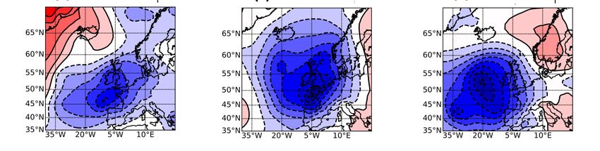
(a) Tregde north-station
NAO+ (100%)
(b) La Coruña south-station
NAO- (40%) (30%) (30%)
Figure 7. Typical weather situations (SLP anomalies) driving the 15 highest storm surges recorded at (a) Tregde
and (b) La Coruña. SLP anomalies are computed from 20CR, retrieving the average value over the period 1836-
2015. See Supplementary Fig. S6 for the corresponding SLP and wind fields.
around 4 days/decade later in the North, and 5 days/decade earlier in the South. Such a tendency is similar to
the one already reported for the European river floods, between 1960 and 2 01038. The floods arrive a few days/
decade earlier in northern Europe (in the North Sea), and a few days per decade later in Southern Europe (along
the Atlantic coasts).
This work could be extended to additional tide gauges. Indeed, in our study we focused on long-term stations
(> 50 years) to investigate the shift over the 1950–2000 period. This led to disregarding many recent stations
(see the small points on Fig. 1). Preliminary results on two of them, Milford Haven along the west coast of Great
Britain and Malin Head in Northern Ireland, confirm the shift.
Concerning possible causes, the high correlation between the timing of the storm surge season and the
NAO first suggests a key role of the large-scale North Atlantic atmospheric circulation. In northern stations,
the seasonal shift was already present in the atmospheric data: between 1950 and 2000, the SLP extremes occur
later, suggesting later winter storms. The same way, Blöschl et al.38 attributed the later river floods in the North
Sea to later winter storms. Possibly, storm surge spatio-temporal shifts may trace changes in the storm tracks,
accompanying NAO changes, to also likely co-vary with surface temperature and precipitation variability in the
North Atlantic sector. Importantly, since the 1990s, the NAO phase is switching from a positive to a negative
phase. Consequently, since 2000, the storm surge season tends to now arrive earlier in the North and later in the
South. In other words, the observed shift between 1950 and 2000 is not a long-term trend but more likely the
signature of large-scale atmospheric decadal variability.
To go further, we investigated the timing of persistent NAO+ and NAO− regimes, through the analysis
of a new index, the NAOP Timing Index. We found that this index is also shifting between 1950 and 2000,
positively for NAOP+ (≈ 3 days/decade), and negatively for NAOP− (≈ -3 days/decade). For the strong NAO+
regimes, causing larger storm surges in northern Europe, the storms tend to arrive later. Reversely, for strong
NAO− regimes, causing larger storm surges in southern Europe, the storms tend to arrive earlier. Note that
this new NAOP timing index may be used as a proxy for changes in the storm surge season, but also for other
parameters, such as precipitation or flooding.
Finally, we classified the typical atmospheric situations generating storm surges at two stations, located in the
North and in the South. Results show that the north-station is clearly characterized by a single typical situation
(NAO+), whereas the south-station is characterized by three typical situations (NAO− and two other situations
close to a Blocking regime). This variety of storms impacting the south-station explains the seemingly poorer
agreement between the timing of the storm surge season and atmospheric extremes in the South of Europe
compared to the North of Europe. Further works will have to be conducted to understand more deeply the
discrepancies in southern Europe. For example, additional analyses could be conducted on the atmospheric
fields, in order to derive indices corresponding to the other situations than NAO, and quantify their influence.
Scientific Reports | (2022) 12:8210 | https://doi.org/10.1038/s41598-022-12356-5 9
Vol.:(0123456789)www.nature.com/scientificreports/
Data availability
The GESLA-2 surge d ataset1,22 analysed during the current study is available on the GESLA-2 website, https://
gesla787883612.wordpress.com/gesla2/, the repository link is in the Bibliography section, following the “Mar-
cos, M. and Woodworth, P.L. 2017.” reference, “Supplementary data is here”, https://drive.google.com/open?id=
0B4lJ8jUz5qwLOXNBLXFtSmdzLXM (last access: May 2020). The winter NAO index is available in the Climate
Analysis Section (NCAR, Boulder, USA) repository, https://climatedataguide.ucar.edu/sites/default/files/nao_
statio
n_d
jfm.t xt (last access: April 2020). The Twentieth Century Reanalysis Project version 3 dataset is available
in the NOAA repository, ftp://ftp2.psl.noaa.gov/Datasets/20thC_ReanV3/ (last access: January 2021).
Received: 4 March 2022; Accepted: 9 May 2022
References
1. Marcos, M. & Woodworth, P. L. Spatiotemporal changes in extreme sea levels along the coast of the North Atlantic and the Gulf
of Mexico. J. Geophys. Res. Oceans 122, 7031–7048. https://doi.org/10.1002/2017JC013065 (2017).
2. Wolf, J. & Flather, R. Modelling waves and surges during the 1953 storm. Philos. Trans. A. Math. Phys. Eng. Sci. 363, 1359–1375.
https://doi.org/10.1098/rsta.2005.1572 (2005).
3. Choi, B. H., Kim, K. O., Yuk, J.-H. & Lee, H. S. Simulation of the 1953 storm surge in the North Sea. Ocean Dyn. 6, 1759–1777
(2018).
4. Bertin, X. et al. A modeling-based analysis of the flooding associated with Xynthia, central Bay of Biscay. Coastal Eng. 94, 80–89.
https://doi.org/10.1016/j.coastaleng.2014.08.013 (2014).
5. Genovese, E. & Przyluski, V. Storm surge disaster risk management: the Xynthia case study in France. J. Risk Res. 16, 825–841.
https://doi.org/10.1080/13669877.2012.737826 (2013).
6. Pineau-Guillou, L. et al. Sea levels analysis and surge modelling during storm Xynthia. Eur. J. Environ. Civ. Eng. 16, 943–952.
https://doi.org/10.1080/19648189.2012.676424 (2012).
7. Hamdi, Y., Bardet, L., Duluc, C.-M. & Rebour, V. Use of historical information in extreme-surge frequency estimation: The case
of marine flooding on the La Rochelle site in France. Nat. Hazards Earth Syst. Sci. 15, 1515–1531. https://doi.org/10.5194/nhess-
15-1515-2015 (2015).
8. Bengtsson, L., Hodges, K. I. & Roeckner, E. Storm tracks and climate change. J. Clim. 19, 3518–3543. https://d oi.o rg/1 0.1 175/J CLI3
815.1 (2006).
9. IPCC. Climate Change 2021: The Physical Science Basis. Contribution of Working Group I to the Sixth Assessment Report of the
Intergovernmental Panel on Climate Change ([Masson-Delmotte, V., P. Zhai, A. Pirani, S. L. Connors, C. Péan, S. Berger, N. Caud,
Y. Chen, L. Goldfarb, M. I. Gomis, M. Huang, K. Leitzell, E. Lonnoy, J.B.R. Matthews, T. K. Maycock, T. Waterfield, O. Yelekçi, R.
Yu and B. Zhou (eds.)]. Cambridge University Press. In Press., 2021).
10. Menendez, M. & Woodworth, P. L. Changes in extreme high water levels based on a quasi-global tide-gauge data set. J. Geophys.
Res. Oceans 115, C10011. https://doi.org/10.1029/2009JC005997 (2010).
11. Marcos, M., Calafat, F. M., Berihuete, A. & Dangendorf, S. Long-term variations in global sea level extremes. J. Geophys. Res. Oceans
120, 8115–8134. https://doi.org/10.1002/2015JC011173 (2015).
12. Haigh, I., Nicholls, R. & Wells, N. Assessing changes in extreme sea levels: Application to the English Channel, 1900–2006. Cont.
Shelf Res. 30, 1042–1055. https://doi.org/10.1016/j.csr.2010.02.002 (2010).
13. Weiss, J., Bernardara, P. & Benoit, M. Formation of homogeneous regions for regional frequency analysis of extreme significant
wave heights. J. Geophys. Res. Oceans 119, 2906–2922. https://doi.org/10.1002/2013JC009668 (2014).
14. Cid, A. et al. Long-term changes in the frequency, intensity and duration of extreme storm surge events in southern Europe. Clim.
Dyn. 46, 1503–1516. https://doi.org/10.1007/s00382-015-2659-1 (2016).
15. Wahl, T. & Chambers, D. P. Evidence for multidecadal variability in US extreme sea level records. J. Geophys. Res. Oceans 120,
1527–1544. https://doi.org/10.1002/2014JC010443 (2015).
16. Wahl, T. & Chambers, D. P. Climate controls multidecadal variability in U. S. extreme sea level records. J. Geophys. Res. Oceans
121, 1274–1290. https://doi.org/10.1002/2015JC011057 (2016).
17. Oey, L.-Y. & Chou, S. Evidence of rising and poleward shift of storm surge in western North Pacific in recent decades. J. Geophys.
Res. Oceans 121, 5181–5192. https://doi.org/10.1002/2016JC011777 (2016).
18. Talke, S. A., Orton, P. & Jay, D. A. Increasing storm tides in New York Harbor, 1844–2013. Geophys. Res. Lett. 41, 3149–3155.
https://doi.org/10.1002/2014GL059574 (2014).
19. Calafat, F. M., Wahl, T., Tadesse, M. G. & Sparrow, S. N. Trends in europe storm surge extremes match the rate of sea-level rise.
Nature 603, 841–845. https://doi.org/10.1038/s41586-022-04426-5 (2022).
20. Feser, F. et al. Storminess over the North Atlantic and northwestern Europe - A review. Q. J. R. Meteorolo. Soc. 141, 350–382. https://
doi.org/10.1002/qj.2364 (2015).
21. Reinert, M., Pineau-Guillou, L., Raillard, N. & Chapron, B. Seasonal shift in storm surges at Brest revealed by extreme value analysis.
J. Geophys. Res. Oceans 126, e2021JC017794. https://doi.org/10.1029/2021JC017794 (2021).
22. Woodworth, P. L. et al. Towards a global higher-frequency sea level dataset. Geosci. Data J. 3, 50–59. https://doi.org/10.1002/gdj3.
42 (2017).
23. Caldwell, P. C., Merrifield, M. A. & Thompson, P. R. Sea level measured by tide gauges from global oceans - the Joint Archive for
Sea Level holdings (NCEI Accession 0019568), Version 5.5. NOAA National Centers for Environmental Information Dataset. https://
doi.org/10.7289/V5V40S7W. (2015).
24. Pugh, D. & Woodworth, P. Sea Level Science: Understanding Tides, Surges, Tsunamis and Mean Sea Level Changes (Cambridge
University Press, Cambridge, 2014).
25. Dangendorf, S., Marcos, M., Wöppelmann, G., Frederikse, C. P. C. T. & Riva, R. Reassessment of 20th century global mean sea
level rise. PNAS 114, 5946–5951 (2017).
26. Chen, X. et al. The increasing rate of global mean sea-level rise during 1993–2014. Nat. Clim. Change 7, 492–495. https://doi.org/
10.1038/nclimate3325 (2017).
27. Hurrell, J. W. Decadal trends in the North Atlantic oscillation—Regional temperature and precipitation. Science 269, 676–679.
https://doi.org/10.1126/science.269.5224.676 (1995).
28. Hurrell, J. W. & Deser, C. North Atlantic climate variability : The role of the North Atlantic Oscillation. J. Mar. Syst. 79, 231–244.
https://doi.org/10.1016/j.jmarsys.2009.11.002 (2010).
29. Compo, G. P. et al. The twentieth century reanalysis project. Q. J. R. Meteorol. Soc. 137, 1–28. https://d
oi.o
rg/1 0.1 002/q j.7 76 (2011).
30. Slivinski, L. C. et al. Towards a more reliable historical reanalysis: Improvements for version 3 of the twentieth century reanalysis
system. QQ. J. R. Meteorol. Soc. 145, 2876–2908. https://doi.org/10.1002/qj.3598 (2019).
31. Reinert, M. Extreme Surge Analysis Codes (v1.1.1). Zenodo. https://doi.org/10.5281/zenodo.5674878 (2021).
32. Coles, S. An Introduction to statistical Modeling of Extreme Values (Springer, Berlin, 2001).
Scientific Reports | (2022) 12:8210 | https://doi.org/10.1038/s41598-022-12356-5 10
Vol:.(1234567890)www.nature.com/scientificreports/
33. Haigh, I. D. et al. Spatial and temporal analysis of extreme sea level and storm surge events around the coastline of the UK. Sci.
Data 3, 160107. https://doi.org/10.1038/sdata.2016.107 (2016).
34. Cassou, C., Terray, L., Hurrell, J. W. & Deser, C. North Atlantic winter climate regimes : Spatial asymmetry, stationarity with time
and oceanic forcing. J. Clim. 17, 1055–1068 (2004).
35. Cassou, CDu. changement climatique aux régimes de temps : l’oscillation nord-atlantique [Prix Prud’homme 2002]. Météorol. 45,
21–32. https://doi.org/10.4267/2042/36039 (2004).
36. D’Andrea, F. Entre le temps et le climat, la variabilité intrasaisonnière de l’atmosphère [Prix Prud’homme 2000]. Météorol. 41,
30–37. https://doi.org/10.4267/2042/36281 (2003).
37. Zubiate, L., McDermott, F., Sweeney, C. & O’Malley, M. Spatial variability in winter NAO-wind speed relationships in western
Europe linked to concomitant states of the East Atlantic and Scandinavian patterns. Q. J. R. Meteorol. Soc. 143, 552–562. https://
doi.org/10.1002/qj.2943 (2017).
38. Blöschl, G. et al. Changing climate shifts timing of the European floods. Science 357, 588–590. https://doi.org/10.1126/science.
aan2506 (2017).
Acknowledgements
This research has been supported by the French National Research Agency (ANR) grant ClimEx (ANR-
21-CE01-0004). It has also been supported by the research theme “Long-term observing systems for ocean
knowledge” of the ISblue project “Interdisciplinary graduate school for the blue planet”, co-funded by a grant
from the French government under the program “Investissements d’Avenir” (ANR-17-EURE-0015). Support
for the Twentieth Century Reanalysis Project version 3 dataset was provided by the U.S. Department of Energy,
Office of Science Biological and Environmental Research (BER), by the National Oceanic and Atmospheric
Administration Climate Program Office, and by the NOAA Physical Sciences Laboratory.
Author contributions
J.B.R. and L.P.G. analysed the data and wrote the paper. B.C. and N.R. discussed the results. M.R. contributed to
the software development used in our analysis. L.P.G. supervised the work. All authors reviewed the manuscript.
Competing interests
The authors declare no competing interests.
Additional information
Supplementary Information The online version contains supplementary material available at https://doi.org/
10.1038/s41598-022-12356-5.
Correspondence and requests for materials should be addressed to J.-B.R.
Reprints and permissions information is available at www.nature.com/reprints.
Publisher’s note Springer Nature remains neutral with regard to jurisdictional claims in published maps and
institutional affiliations.
Open Access This article is licensed under a Creative Commons Attribution 4.0 International
License, which permits use, sharing, adaptation, distribution and reproduction in any medium or
format, as long as you give appropriate credit to the original author(s) and the source, provide a link to the
Creative Commons licence, and indicate if changes were made. The images or other third party material in this
article are included in the article’s Creative Commons licence, unless indicated otherwise in a credit line to the
material. If material is not included in the article’s Creative Commons licence and your intended use is not
permitted by statutory regulation or exceeds the permitted use, you will need to obtain permission directly from
the copyright holder. To view a copy of this licence, visit http://creativecommons.org/licenses/by/4.0/.
© The Author(s) 2022
Scientific Reports | (2022) 12:8210 | https://doi.org/10.1038/s41598-022-12356-5 11
Vol.:(0123456789)You can also read