Simulazione Diretta di una Fiamma Premiscelata Metano/Idrogeno/Aria
←
→
Page content transcription
If your browser does not render page correctly, please read the page content below

Agenzia nazionale per le nuove tecnologie,
l’energia e lo sviluppo economico sostenibile                                                  MINISTERO DELLO SVILUPPO ECONOMICO


                                                 Simulazione
  Diretta
  di
  una
  Fiamma

                                                Premiscelata
  Metano/Idrogeno/Aria


         D.
  Cecere,
  E.
  Giacomazzi,
  F.R.
  Picchia,
  N.
  Arcidiacono


                                                                                           Report
  RdS/PAR2013/270

SIMULAZIONE
DIRETTA
DI
UNA
FIAMMA
PREMISCELATA
METANO/IDROGENO/ARIA
D.
Cecere,
E.
Giacomazzi,
F.R.
Picchia,
N.
Arcidiacono,
(ENEA,
UTTEI-‐COMSO)
Settembre
2014
Report
Ricerca
di
Sistema
Elettrico
Accordo
di
Programma
Ministero
dello
Sviluppo
Economico
–
ENEA
Piano
Annuale
di
Realizzazione
2013
Area:
Produzione
di
energia
elettrica
e
protezione
dell'ambiente
Progetto:
B.2
-‐
Cattura
e
sequestro
della
CO2
prodotta
dall'utilizzo
di
combustibili
fossili
Obiettivo:
Parte
A
-‐
b
-‐
Tecnologie
per
l'ottimizzazione
dei
processi
di
combustione
Task
b.1
-‐
Metodologie
numeriche
avanzate
per
la
simulazione
dei
processi
di
combustione
e
la
progettazione
di
componenti
Responsabile
del
Progetto:
Stefano
Giammartini,
ENEA
Indice

Summary                                                                                                                                                                        4

1   Introduction                                                                                                                                                               5
    1.1   Problem configuration . . . . . . . . . . . . . . . . . . . . . . . . . . . . . . . . . . . . . .                                                                     5
    1.2   Governing Equations . . . . . . . . . . . . . . . . . . . . . . . . . . . . . . . . . . . . . . .                                                                     6
          1.2.1 Physical Properties and Kinetic Model . . . . . . . . . . . . . . . . . . . . . . . . . .                                                                       7

2   Numerical Results                                                                                                                                                          12
    2.1   General characteristics of the flame .   .   .   .   .   .   .   .   .   .   .   .   .   .   .   .   .   .   .   .   .   .   .   .   .   .   .   .   .   .   .   .   12
    2.2   Displacement speeds . . . . . . . .      .   .   .   .   .   .   .   .   .   .   .   .   .   .   .   .   .   .   .   .   .   .   .   .   .   .   .   .   .   .   .   12
    2.3   Flame thickness and curvature . . .      .   .   .   .   .   .   .   .   .   .   .   .   .   .   .   .   .   .   .   .   .   .   .   .   .   .   .   .   .   .   .   18
    2.4   Conclusions . . . . . . . . . . . . .    .   .   .   .   .   .   .   .   .   .   .   .   .   .   .   .   .   .   .   .   .   .   .   .   .   .   .   .   .   .   .   18

                                                                                                                                                                                3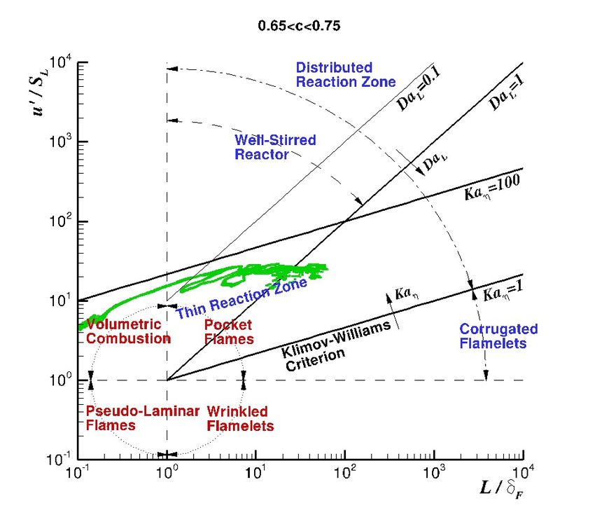
Accordo di PROGRAMMA MSE-ENEA

Sommario
Negli ultimi anni, grazie all’avvento di computer ad alte prestazioni e avanzati algoritmi numerici, la simula-
zione numerica diretta (DNS) della combustione é emersa come un valido strumento di ricerca insieme alla
sperimentazione. Per comprendere l’influenza della turbolenza sulla struttura della fiamma, in questo lavoro
si effettuata una DNS tridimensionale di una fiamma premiscelata magra CH4 /H2 -Aria. Il regime di fiamma
premiscelata é quello del Thin Reaction Zone. Si é utilizzato uno schema cinetico dettagliato per la chimica
del Metano-Aria costituito da 22 specie e 73 reazioni elementari. Inoltre per la discretizzazione spaziale delle
equazioni é stata adottato uno schema al sesto ordine compatto sviluppato in ENEA per flussi comprimibili e
griglie staggerate. Sono state calcolate in fase di post processing le velocit di spostamento del fronte di fiamma
(individuato da isosuperfici di variabile di progresso) in funzione delle curvature e dello strain-rate e le probabi-
lity density function (PDF) di queste grandezze. Nello studio delle caratteristiche della fiamma sono state prese
in considerazione le diverse diffusivit delle diverse specie chimiche costituenti la miscela. É stata sviluppata
una nuova formulazione delle velocit di spostamento delle isosuperfici della variabile di progresso che tiene in
conto delle diverse diffusivit delle specie chimiche.

4
1 Introduction

In many practical devices for power generation, such as stationary gas turbines, or propulsive systems, there
has been a strong interest in achieving more efficiency and low polluttants emissions. For this purpose lean
combustion burners are developed. The advantages of operating at lean mixture conditions are high thermal
efficiency and low emissions of NOx due to lower ame temperatures. Unfortunately at leaner conditions the
flame tends to be thicker and propagate more slowly, suffering of flame instability. Local flame extinction
occurs as a consequence of lean combustion conditions associated with stretching and heat losses. In order to
overcome this issue, it possible increase the laminar burning velocity adding a small percentage of hydrogen to
the lean premixed methane/air flame mixture. The hydrogen’s large laminar burning velocity (approximately
7 times that of methane at 300 K and 1 bar) and the wider flammability limits allows the extension of the
operational range of the combustion system. However, hydrogen is less energy dense than all other fuels,
resulting in a loss of power in proportion to the base fuel substituted. For turbulent flames with hydrogen added
to methane the literature is limited; we mention the experimental studies of [1, 4] and the two-dimensional DNS
(with a chemical mechanism reduced to 19 species and 15 reactions) by Hawkes and Chen [5]. The topic of
hydrogen addition has become important recently, in particular because of the need to increase the knowledge
about the effects of biomass and coal gasication and addition of the obtained and shifted gases to regular fuels.

1.1 Problem configuration
The simulation was performed in a slot-burner Bunsen flame configuration. The slot-burner Bunsen configu-
ration is especially interesting due to the presence of mean shear in the flow and is similar in configuration to
the burner used in experimental studies [6]. This configuration consists of a central reactant jet through which
premixed reactants are supplied. The central jet is surrounded on either side by a heated coflow, whose com-
position and temperature are those of the complete combustion products of the freely propagating jet mixture.
The reactant jet was chosen to be a premixed methane/hydrogen air jet at 600 K and mixture equivalence ratio
φ = 0.7, with molar fractional distribution of 20% H2 and 80% CH4 . The unstrained laminar flame properties at
these conditions computed using Chemkin [16] are summarized in Table 1.1. In this table φ represents the mul-
ticomponent equivalence ratio of the reactant jet mixture, φ = [(XH2 + XCH4 )/XO2 ]/[(XH2 + XCH4 )/XO2 ]stoich ,
Tu is the unburned gas temperature, Tb the products gas temperature, sL represents the unstrained laminar fla-
me speed and δth = (Tb − Tu )/|∂T/∂x|max is the thermal thickness based on maximum temperature gradient.
Preheating the reactants leads to a higher flame speed and allows a higher inow velocity without blowing out
the flame, reducing computational costs. Also, many practical devices such as gas turbines, internal combu-
stion engines, and recirculating furnaces operate at highly preheated conditions. The simulation parameters are
summarized in Table 1.2.
   The domain size in the streamwise (z), crosswise (y) and spanwise (x) directions is L x × Ly × Lz = 24h ×
15h × 2.5h, h being the slot width (h = 1.2mm). The grid is uniform only in the x direction (∆x = 20µm),
while is stretched in the y and z direction near the inlet duct walls. The DNS was run at atmospheric pressure

                        φ    nH2 = xH2 /(xH2 + xCH4 )   Tu [K]   Tb [K]   sL [cm s−1 ]   δth [mm]
                       0.7             0.2               600     2072       103.75        0.3476

                                   Tabella 1.1: CH4 /H2 − Air laminar flame.

                                                                                                               5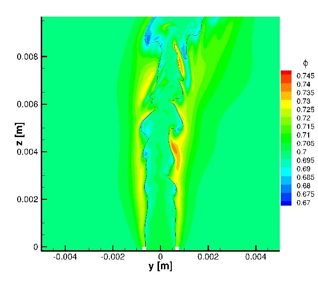
Accordo di PROGRAMMA MSE-ENEA

                           Slot width (h)                                    1.2 mm
                           Domain size in the spanwise (Lx ), crosswi-   24h × 15h × 2.5h
                           se (Ly ) and streamwise (Lz ) directions
                           N x × Ny × Nz                                 1550 × 640 × 140
                           Turbulent jet velocity (U0 )                     110 m s−1
                           Coflow velocity                                   25 m s−1
                           Jet Reynolds Number (Re jet = U0 h/υ)               2264
                           Turbulent intensity (u0 /S L )                      12.5
                           Turbulent length scale (lt /δL )                     2.6
                           Turbulent Reynolds Number (Ret =                     226
                           u0 ηK /υ)
                           Damkohler number (sL Lt /u0 L)                     0.21
                           Karlovitz number (δL /ηK )                         503
                           Minimum grid space                                 9 µm
                           Kolmogorov Lenght Scale ηK                       17.22 µm

Tabella 1.2: CH4 /H2 − Air turbulent flame: the kinematic viscosity used in the calculation of Reynolds number
             is that of the inflow CH4 − H2 /Air mixture ν = 5.3 · 10−5 m2 s−1

using a 17 species and 73 elementary reactions kinetic mechanism [7]. The velocity of the central jet stream
is 100 m/s, while the velocity of the coflow stream is 25 m/s. The width h of the central duct, where the
inlet turbulent velocity profile may develop, is 1.2 mm and 4 mm long. The width walls of the duct hw is
0.18 mm. Velocity fluctuations, u0 = 12 m s−1 , are imposed on the mean inlet velocity profile, obtained by
generating at duct’s inlet homogeneous isotropic turbulence field with a characteristic turbulent correlation
scale in the streamwise direction of δcorr = 0.0004 m and a streamwise velocity fluctuation of u0z = 12 ms−1 ,
are imposed on the mean inlet duct’s velocity profile by means of Klein’s procedure [8]. The jet Reynolds
number based on the centerline inlet velocity and slot width h is Rejet = Uh/υ = 2264. Based on the jet
exit duct centerline velocity and the total streamwise domain lenght, the flow through time is τU = 0.218 ms.
Navier-Stokes characteristic boundary conditions (NSCBC) were adopted to prescribe boundary conditions.
Periodic boundary conditions were applied in the x direction, while improved staggered non-reflecting inflow
and outflow boundary conditions were fixed in y and z directions [9, 10]. The simulation was performed
on the linux cluster CRESCO (Computational Center for Complex Systems) at ENEA, requiring 1.5 million
CPU-hours running for 20 days on 3500 processors. The solution was advanced at a constant time step of 2.3 ns
and after the flame reached statistical stationarity, the data were been collected through 4 τU .

1.2 Governing Equations
In LES each turbulent field variable is decomposed into a resolved and a subgrid-scale part. In this work, the
spatial filtering operation is implicitly defined by the local grid cell size. Variables per unit volume are treated
using Reynolds decomposition, while Favre (density weighted) decomposition is used to describe quantities
per mass unit. The instantaneous small-scale fluctuations are removed by the filter, but their statistical effects
remain inside the unclosed terms representing the influence of the subgrid scales on the resolved ones. In this
article, a test deals with combustion to show the robustness of the suggested technique. Gaseous combustion
is governed by a set of transport equations expressing the conservation of mass, momentum and energy, and
by a thermodynamic equation of state describing the gas behaviour. For a mixture of N s ideal gases in local
thermodynamic equilibrium but chemical nonequilibrium, the corresponding filtered field equations (extended
Navier−Stokes equations) are:

    • Transport Equation of Mass
6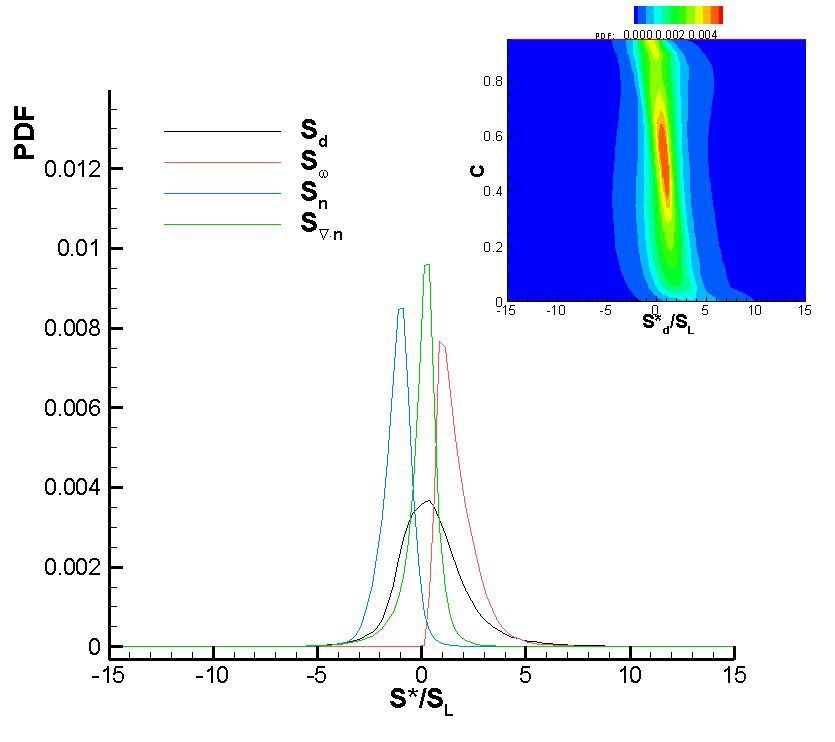
∂ρ ∂ρui
                                                         +     = 0.                                            (1.1)
                                                      ∂t   ∂xi

   • Transport Equation of Momentum

                                            ∂(ρu j ) ∂(ρui u j + pδi j ) ∂τi j
                                                    +                   =                                      (1.2)
                                              ∂t            ∂xi           ∂xi

   • Transport Equation of Total Energy (internal + mechanical, E + K)

                                       ∂(ρ U) ∂(ρui U + pui )    ∂(qi − u j τi j )
                                             +                =−                                               (1.3)
                                         ∂t         ∂xi               ∂xi

   • Transport Equation of the N s Species Mass Fractions

                                         ∂(ρ Yn ) ∂(ρu j Yn )     ∂
                                                 +            = − (Jn,i ) + ω̇n                                (1.4)
                                           ∂t        ∂xi         ∂xi

   • Thermodynamic Equation of State
                                                             Ns
                                                            X   Yn
                                                    p=ρ            Ru T                                        (1.5)
                                                            n=1
                                                                Wn

These equations must be coupled with the constitutive equations which describe the molecular transport. In
the above equations, t is the time variable, ρ the density, u j the velocities, τi j the viscous stress tensor, U the
total filtered energy per unit of mass, that is the sum of the filtered internal energy, ee, and the resolved kinetic
energy, 1/2 ui ui , qi is the heat flux, p the pressure, T the temperature, Ru is the universal gas constant, Wn the
nth-species molecular weight, ω̇n is the production/destruction rate of species n, diffusing at velocity Vi,n and
resulting in a diffusive mass flux J n = ρYn V n. The stress tensor and the heat flux are respectively:

                                                               1
                                             τi j = 2µ (S i j − S kk δi j )                                    (1.6)
                                                               3
                                                           Ns
                                                   ∂T     X
                                           qi = −k     +ρ     hn Yn Vi,n .                                     (1.7)
                                                   ∂xi    n=1

In Eqn. 1.6-1.7 µ is the molecular viscosity and k is the termal conductivity.
   The simulation were performed using the code HeaRT, which solves the fully compressible Navier-Stokes,
species and total energy equations (1.1-1.4) with the fully explicit third-order accurate TVD Runge-Kutta sche-
me of Shu and Osher [21] and a sixth order compact staggered scheme for non-uniform grid (with the non
uniform grid effects included in the compact coefficients scheme). No filter is necessary for ensuring stable so-
lutions [22, 23, 24]. Fig. 1.1 shows the computational domain adopted in the simulation with a slice indicating
the not uniform grid in the streamwise and crosswise directions (only one grid line each ten is represented), and
the different stencils (due to the presence of walls and non periodic outlet) of the staggered compact scheme in
the three coordinates directions.

1.2.1 Physical Properties and Kinetic Model
Kinetic theory is used to calculate dynamic viscosity and thermal conductivity of individual species [14]. The
mixture-average properties are estimated by means of Wilke’s formula with Bird’s correction for viscosity
[15],[16], and Mathur’s expression for thermal conductivity [17].
   Eqn. 1.7, the first term is the heat transfer by conduction, modeled by Fourier’s law, the second is the heat
transport due to molecular diffusion acting in multicomponent mixtures and driven by concentration gradients.
                                                                                                                   7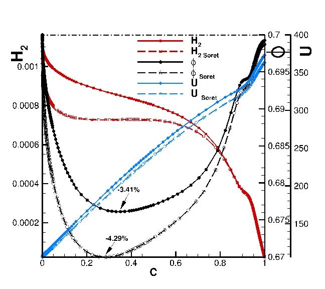
Accordo di PROGRAMMA MSE-ENEA

                           h!

Figura 1.1: Slice of instantaneous streamwise velocity with not uniform computational grid (for clarity only
            one grid line each ten is represented). Coloured arrows: the compact finite difference stencils in the
            three directions for each zone of the computational domain; Isosurface of temperature T = 700.

The Hirschfelder and Curtiss approximate formula for mass diffusion V n in a multicomponent mixture and
Soret effect are adopted, i.e.,
                                                             Ns
                                                                                    ∇T
                                                                   D?n j dn − DTn
                                                             X
                                     J n = ρYn V n = −ρYn
                                                                                     T
                                                             i=1                                              (1.8)
                                             Wn                ∇T
                                        = −ρ      Dn ∇Xn − DTn    ,
                                             Wmix              T
    with Xn = Yn Wmix /Wn and the Dn is
                                                       1 − Yn
                                               Dn = P         Xj
                                                                 .                                            (1.9)
                                                      Ns
                                                          j=1, j,n D jn

D jn being the binary diffusion coefficient and DTn is the n-th species thermo diffusion coefficient and dn the
diffusional driving forces that for low-density gases became:
                                                                 Ns
                                                          ∇p ρ X
                                 d n = ∇Xn + (Xn − Yn )                Yi Yn ( f i − f n )                   (1.10)
                                                           p p i=1,i,n
   Only the first cross diffusion term of Eqn. 1.10 is retained in this work, while the pressure gradient diffusion
(low subsonic flame flow) and the external forces diffusion (low-density gases assumption) are neglected.
   Soret effect is due to the fact that for hard molecules, with interacting forces varying with distance more
strongly than the inverse of the fifth power, there is a larger transfer of momentum in collisions with larger
relative velocity of the colliding partners. For molecules of different masses, since the thermal agitation velocity
of the i-th species is proportional to (T/mi )1/2 , there will be more collisions with large relative velocity with
lighter molecules coming from the hotter region and heavier coming from the colder than vice versa. The net
transfer of momentum from heavy to light molecules is then directed towards the hotter part of the gas and the
thermal diffusion ratio of light species is negative [19],[18]. Light molecules will have a tendency to stay in hot
zone and leave cold zones and vice versa.
   When inexact expressions for diffusion velocities are used (as when using Hirschfelder’s law), and in general
                                                                     PN s       PN s
when differential diffusion effects are considered, the constrain i=1     J i = i=1   ρYi Vi = 0 is not necessarily
satisfied. In this paper, to impose mass conservation, an artificial diffusion velocity V c is subtracted from
8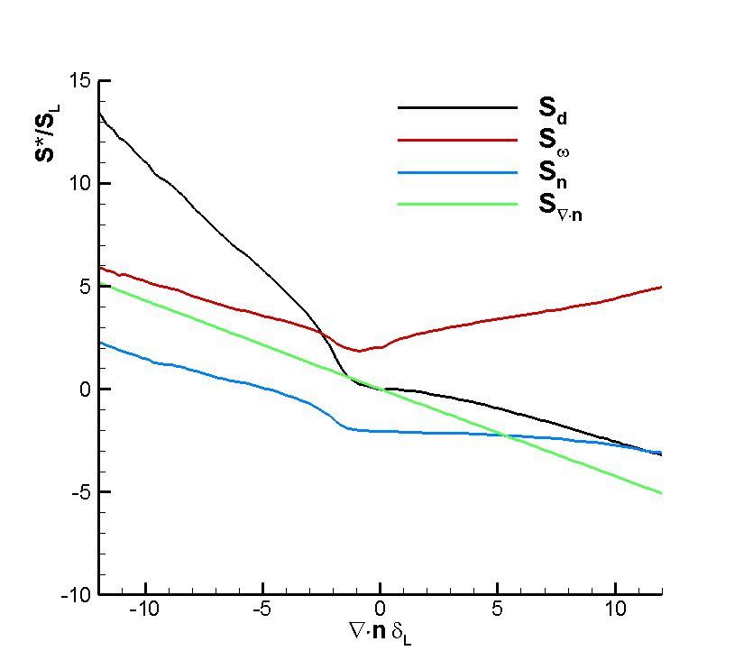
Figura 1.2: Comparison of species mole fraction in the detailed and reduced kinetic schemes: solid line)
            GRIMECH 3.0 kinetic scheme [11]; Long dashed line) Reduced kinetic scheme [7].

the flow velocity in the species transport equations [12]. This velocity, assuming Hirschfelder’s law holds,
becomes:
                                                   Ns
                                                  X    Wn
                                           V =−
                                            c              Dn ∇Xn .                                   (1.11)
                                                  n=1
                                                      Wmix

   Fig. 1.2-1.3 show freely propagating premixed (Φ = 0.7) flame results obtained with the detailed (GRIMECH
3.0 [11]) and reduced kinetic scheme without the inclusion of the Soret effect (Eqn. 1.8) obtained by means of
CHEMKIN code [16]. The thermochemical information on the gas phase and the Lennard Jones coefficients
for the evaluation of transport properties were obtained primarily from the CHEMKIN database [16]. The
maximum errors of the reduced scheme are ∼ 4% and ∼ 6% for the laminar flame velocity and temperature
respectively.
   Fig. 1.4 shows the gradient of temperature and the heat release in the normalized progress variable space c.
The progress variable Yc is defined as the sum of CO, CO2 , H2 O mass fractions while the :

                                                       Yc − Yc,b
                                                 c=                                                        (1.12)
                                                      Yc, f − Yc,b
   where Yc, f and Yc,b are the proegress variable mass fractions in the fresh and burned gas respectively. The
heat release is complete at c ∼ 0.9. The maximum heat release is at c = 0.704, while the maximum value of
temperature gradient, adopted for the calculation of laminar thermal thickness δth , is at c = 0.44.
   Fig.1.5 shows the effects of preferential diffusion and Soret effect on the structure of the premixed laminar
flames in the progress variable space. For the flame considered the only elements present are carbon, hydrogen,
oxygen and nitrogen: m = C, H, O, N and the local equivalence ratio φ is calculated as:

                                                    2AC + 0.5AH
                                               φ=                                                          (1.13)
                                                        AO
   where Am = k=1      αk,m xk is the number of moles of atom of element m per mole of gas, αk,m the number of
                 PK
atoms of element m per species k and xk its mole fraction. Since chemical reactions do not change the elemental
composition, and convection in an ideal one-dimensional system merely translates fluid without affecting its
composition, variation of elemental composition with respect to distance in the freely propagating flame occurs
as a result of axial differential diffusion of initial reactants, the major products and key intermediates such H.
                                                                                                                9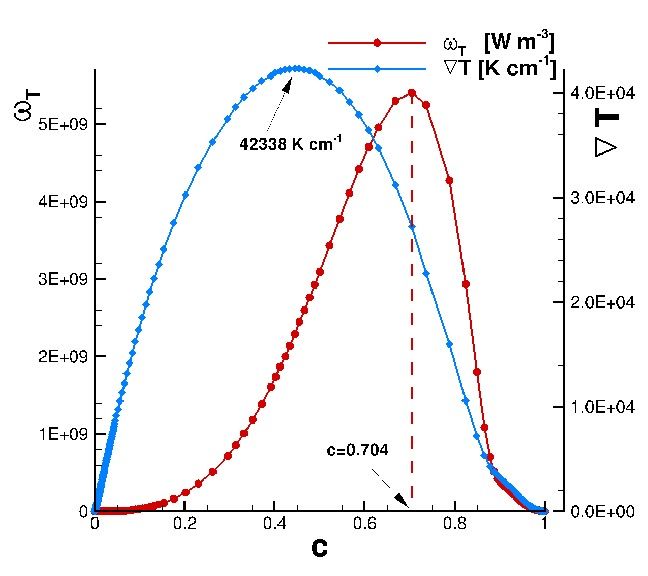
Accordo di PROGRAMMA MSE-ENEA

Figura 1.3: Comparison of velocity and temperature in the detailed and reduced kinetic schemes: solid line)
            GRIMECH 3.0 kinetic scheme [11]; Long dashed line) Reduced kinetic scheme [7].

Figura 1.4: Temperature gradient (bullets) and heat reaction rate (squares) of unstretched premixed flame in
            progress variable space.

10
Figura 1.5: Laminar premixed flame solution in progress variable space: Solid lines) Without Soret effect
included; LongDashed lines) With Soret effect included; Dot-Dashed line) Nominal inlet value
equivalence ratio.
Calculated values of φ are shown in Fig.1.5, in the region of maximum temperature gradient the equivalence
ratio decreases to φ ∼ 0.675 (the nominal inlet equivalence ratio φ = 0.7 is indicated as an horizontal dot-dashed
line).
Fig.1.5 shows also that the inclusion of the Soret effect in the laminar flame calculations decrease the local
equivalence ratio and the flame velocity. In fact, since the thermal diffusion coefficients of molecular H2 ,
atomic hydrogen H and O, OH are negative, active radicals and deficient reactant are less prone to diffuse in
the cold region and flame propagation velocity is lower (∼ 3%). Although thermal diffusion as a single eect
tends to drive H2 towards the hot ame region, the nonlinear coupling between transport and chemistry results in
the opposite effect, i.e., the H2 concentration is actually lower in the hot ame region when thermal diffusion is
included in the model. When the deficient reactant is more diffusive than heat (as in the case of H2 ), any portion
of a tridimensional premixed flame protruding into the fresh mixture (convex flame front) burn more vigorously
because diffusive focusing of reactants into the flame is more rapid than heat diffusion away from the bulging
front [25, 26]. Thermal diffusion (Soret effect) supplements the diffusive flux of fuel into the hot reaction zone,
increasing the H2 focusing effect and consequently the effective richness of the mixture in convex zones of the
flame. These last two aspects will be quantified in the following sections.
11Accordo di PROGRAMMA MSE-ENEA
2 Numerical Results
2.1 General characteristics of the flame
An overall description of the slot flame is given by the evolution, downstream the inlet channel, of the axial and
ez , U
radial velocities U ey and their fluctuations shown in Fig. 2.1-2.3. The symbol eφ indicates Favre mean of the
variable φ defined as e φ(y, z) = ρφ/ρ, where ρ is the density and the overbar denotes ensemble averages defined
as:
Nd XNx
1 X
φ(y, z) = φ(xk , y, z, tn ). (2.1)
Nd N x n=1 k=1
with Nd is the number of data sets in a statistically stationary time period (approximately ∼ 8T c = Lz /U0 ),
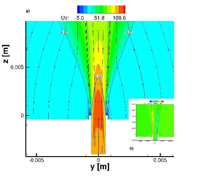
Nd is the number of grid points in the x periodic direction. At the exit of the channel, the axial velocity Uz reach
a maximum value of 110ms−1 greater than its inlet value, due to formation of the channel boundary layer, that
is equivant to a restriction of the flow section (see Fig.2.1).
Downstream, a crosswise component is generated in the coflow because of the presence of the central jet
core (see streamlines in Fig.2.1 and Uy velocity profiles in Fig.2.2b). The blue lines indicates the flame brush
thickness identified using a value of progress variable c between (0.05 − 0.95). The Fig.2.1b shows the mean
shear layer, defined as the velocity gradient in the crosswise direction, and the flame front location, identified
with a value of c = 0.7 corresponding to the location of the maximum heat release of the unstrained laminar
flame (see Fig. 1.4). Due to the presence of wall channel the maximum velocity gradient is located near the
internal edges. The average flame front resides outside of the core of the jet near the wall duct and at 0.009mm
moves towards the inside of the shear layer. The effect of the mixture jet expansion at the exit of channel and
the coflow entrainement towards the jet core is evidenced in Fig. 2.2b (solid line). The velocity fluctuation
is highest in the middle of the shear layer due to the mean shear of the jet and to the heat released by the
flame, reach its maximum value at z ∼ 0.007m and it decreases downstream. These variation of turbulent
characteristics and the development of the flame downstream in the jet suggest that, in order to characterize
the position of the flame in the premixed combustion regime diagram, the local turbulent lenght scale lt , flame
thickness δF and flame velocity S L must be calculated. Here lt = u03 /˜ , with ˜ the average turbulent kinetic
PN s
dissipation rate, δF = (ατch )1/2 , and S L = (ατch )1/2 , with τch = ρc p T/| n=1 Hn ωn |.
Many modeling approaches, describe turbulent premixed flames as an ensemble of flame elements that re-
semble steadily propagating strained or curved laminar flames. When Karlovitz (Ka) number is between 1 and
100 small eddies can penetrate the diffusion preheating zone of the flame and increasing the mixing process, but
not the thinner reaction layer that remains close to a wrinkled laminar reaction zone. This regime is identified
as Thickened Reaction Zone (TRZ) regime. Fig.2.4, show the analysis that places the flame in the TRZ regime,
results that will be confirmed later in the work, by analyzing some statistical properties of the flame.
2.2 Displacement speeds
Under the assumptions that a turbulent premixed flame retains locally the structure of a laminar flame but stret-
ched and wrinkled by the serrounding turbulence, it is possible to separate the non linear nature of turbulence
with that of the reaction rate defining a reaction progress variable, monotonically varying from 0 in the fresh
reactants to 1. The flame zones are identified with progress variable isosurfaces, on which statistics are extrac-
ted. Once the species that define the normalized progress variable c = ( i∈S Yi − i∈S Yi,u )/( i∈S Yi,b − i∈S Yi,u ),
P P P P
12Figura 2.1: Mean streamwise velocity contour plot at the x = 0 plane. Also shown in the contour plot are the ve-
c = 0.05 − 0.95, indicating theh mean flame brush. b)The
locities streamlines and the iso-contour of e
bottom right shows a zoomed in view of the velocity gradient dU ez /dy contour and the iso-contour
of progress variable c̃ = 0.7.
Figura 2.2: a) Mean streamwise velocity Uz versus crosswise direction y; b) Mean crosswise velocity Uy versus
crosswise direction y.
13Accordo di PROGRAMMA MSE-ENEA
Figura 2.3: a) Mean streamwise rms-velocity U0z versus crosswise direction y; b) Mean crosswise velocity U0y
versus crosswise direction y.
Figura 2.4: Borghi diagram.
14are determined (in this case S={CO2 , CO, H2 O}), and considering that Differential Diffusion is taken into ac-
count and Hirschfelder and Curtiss formula for mass diffusion and Soret effect are included (Eqn.1.8), the
classical governing transport equation must be revised as:
∂c 1X Wi
+ u · ∇c = ∇ · (ρ Di ∇Xi )+
∂t ρ i∈S Wm
(2.2)
1X DT ω̇c
∇ · ( i ∇T ) +
ρ i∈S T ρ
with Wm the average mixture molecular weight. The mass diffusion term of Eqn. 2.2 based on the Hirschfel-
der and Curtiss formula may be split into a normal and tangential term recognizing that
Wm Yi
∇Xi =
∇Yi + ∇Wm (2.3)
Wi Wi
with ∇Yi = −|∇Yi |n. Further expansion of the divergence operator, ∇ · (), yields for Eqn.2.2 to:
∂c
+ u · ∇c =
∂t
1 X ρDi Yi
(−n · ∇(ρDi |∇Yi |) − ρDi |∇Yi |∇ · n + ∇ · ( ∇Wm ))+
ρYc,Max i∈S Wm (2.4)
1 X DTi ω̇c
∇·( ∇T ) +
ρYc,Max i∈S
T ρ
Here, ∇ · n is the curvature which may be expressed as the sum of the local inverses of the principal radii of
curvature of the isosurface and flame surface curved convex towards the reactants is assumed to have positive
curvature. The same equation can be written in kinematic form for a progress variable isosurface c = c∗ [27]:
∂c
+ u · ∇c]c=c∗ = S d |∇|c=c∗
[ (2.5)
∂t
where S d , the displacement speed, is the magnitude of the propagation velocity of the isocontour with normal
n = −(∇c/|∇c|)c=c∗ directed toward the unburnt gas. Considering Eqns. (2.2-2.5) the following expression for
the displacement speed S d is obtained:
1
Sd = [ (ωc +
ρ|∇c|Yc,Max
X
(−n · ∇(ρDi |∇Yi |))+
i∈S
X
(−ρDi |∇Yi |∇ · n)+
i∈S (2.6)
X ρDi Yi
(∇ · ( ∇Wm ))+
i∈S
Wm
X DTi
∇·( ∇T ))]c=c∗ .
i∈S
T
This expression shows that S d = S r +S n +S t +S h +S td is determined by the contributions of five contributions:
(a) reaction of progress variable, (b) normal mass diffusion, c) tangential mass diffusion, d) a new term related to
Hirschfelder and Curtiss formula for mass diffusion, e) thermal diffusion. The value of the displacement speed
changes across the flame normal because of thermal expansion effects, using a density-weighted displacement
speed S d∗ = ρS d /ρu this effect may be largely reduced.
15Accordo di PROGRAMMA MSE-ENEA
Figura 2.5: Density weighted mean displacement speed plotted against normalized curvature at c=0.7.
Figure 2.5 shows the density weighted mean (averaged on intervals of curvature) displacement speed and
its components plotted against normalized curvature at isosurface c = 0.7. Curvature and flame displacement
speed are negatively correlated and the flame is thermally stable. Flame elements with negative curvatures
(curvature center in the unburnt mixture) propagate with faster flame speed than positively curved elements.
Even though the local equivalence ratio decrease at negative curvature, due to preferential diffusion of H2
towards hot regions, the effect of heat focusing at negative curvature increases the reaction rate of CH4 , as it has
shown in Fig. 2.6, and consequently the isosurface displacement speed (that is related to reaction rate through
Sr component).
Figura 2.6: Instantaneous heat release [W m-3] contour map and zoomed in view of the CH4 reaction rate. The
maximum of heat release is located at negative curvatures.
The local enrichment of the flame at positive curvature is shown also in Fig.2.7 where the instantaneous
equivalence ratio, calculated with Eqn. 1.13, is shown. While in the laminar flame, the effect of the differential
16diffusion is only a reduction towards leaner condition of the equivalence ratio, in the tridimensional DNS, the
effect of positive curvature produces also local enrichment of the flame.
Figura 2.7: Instantaneous snapshot of the equivalence ratio φ calculated with Eqn.1.13 and isoline of progress
variable c = 0.7.
In Fig. 2.5 it is evident that the flame is thermally stable, since the displacement speed of convex curvature
regions is smaller than that of negative ones. Figure 2.8 shows the Probability Density Function (PDF) of the
normalized density weighted mean displacement speed S d∗ /S L and its components at c = 0.7. At c = 0.7, where
the heat release is maximum, the total Sd is not symmetric around zero, with a skewness towards positive values
of displacement speed and its peak is S s ∼ 1ms−1 .
Figura 2.8: a) PDF of the density weighted mean displacement speed S d∗ /S L and its three components at c=0.7;
b) PDF of S d∗ /S L as a function of c.
In the pre-heating zone of the flame (c < 0.5) the PDF presents a broader range of velocities, thus implying
17Accordo di PROGRAMMA MSE-ENEA
non parallel iso-c surfaces in agreement with the Thin Reaction Regime, where small eddies may affect the
pre-heating zone more than the reaction layer.
2.3 Flame thickness and curvature
In this section the effect of turbulence on flame stirring is studied. The magnitude of the progress variable,|∇c|
is adopted here as a measure of the flame thickness. Figure 2.9 shows the conditional mean of normalized |∇c|
(the laminar flame thickness δL is used as normalizing factor).
Figura 2.9: Conditional means of |∇c| versus progress variable at different heights in the turbulent flame.
The results show that the flame thickness calculated as the inverse of the magnitude of the gradient of progress
variable ∼ 1/|∇c| is lower than the laminar flame thickness δL . It decreases up to an height of 2.4mm in the
flame and then it increases downstream. This is due to the development of the shear layer near the exit of
the mixture channel and to the local increase of the strain rate that reduce the thickness of the flame. Going
downstream the gradient of the velocities in the crosswise direction decreases and the flame thickness increases.
The flame thickening found in this study is in agreement with some experimental results [28].
Figure 2.10 shows mean normalized curvature at different heights in the flame and c = 0.7. The distribution
of curvatures is not symmetric about zero, it has longer tail for positive curvature and its maximum shifts
towards negative curvature moving downstream from the injection channel.
Figure 2.11 shows the PDF of normalized curvature as a function of the progress variable. It is seen that the
distribution of curvature has a negative peak value in the reaction zone (c > 0.5) while this peaks tend to reach
positive values in the diffusion layer (c < 0.5).
2.4 Conclusions
A 3D slot CH4 − H2 /Air flame was simulated with a high-order compact staggered numerical scheme and de-
tailed chemical mechanism. Displacement speeds as function of curvature are examined. Preferential diffusion
of H2 into positively curved flame elements are evidenced, the effect of mass differential diffusion calculated
with the Hirschfelder formula was included in the displacement speed and a new expression was found for the
displacement speed in the case of differential diffusion for the species. The lean flame is intrinsically stable
as shown by the displacement speed as a function of the curvatures, since negative curvature flame elements
present higher velocity than positive ones. Further work is necessary to understand quantitative effect of H2 on
structure of the flame. The simulation of the same flame with the Soret effect included in the transport equations
18Figura 2.10: Probability density function of normalized curvature at different heights in the turbulent flame.
Figura 2.11: Probability density function of normalized curvature in function of the progress variable c in the
turbulent flame.
is actually running on the CRESCO supercomputer cluster. The analysis done for the flame must be repeated
for these results in order to quantify the role of thermal diffusion on statistics and stability of the flame.
19Bibliografia
[1] R.W. Schefer, D.M. Wicksall, A.J. Agrawal, Combustion of hydrogen-enriched methane in a lean
premixed swirl stabilized burner. Proc. Comb. Inst. 2003;29:843-51.
[2] F. Cozzi, A. Coghe, Behavior of hydrogen-enriched non-premixed swirled natural gas flames. Int J.
Hydrogen Energy 2006;31:669-77.
[3] C. Mandilas, M.P. Ormsby, C.G.W. Sheppard, R. Woolley, Effects of hydrogen addition on laminar and
turbulent premixed methane and iso-octaneair flames, Proc. Combust. Inst. 2007;31:1443-50.
[4] F. Halter, C. Chauveau, I. Gokalp, Characterization of the effects of hydrogen addition in premixed
methane/air flames. Int J Hydrogen Energy 2007;32:2585-92.
[5] E.R. Hawkes, J.H. Chen, Direct numerical simulation of hydrogen-enriched lean premixed Methane-Air
Flames, Combust. Flame 138 (2004) 242-58.
[6] S.A. Filatyev, J.F. Driscoll, C.D. Carter, J.M. Donbar, Measured properties of turbulent premixed Flames
for model assessment, including burning velocities, stretch rates, and surface densities, Combust. Flame
141, 1-21, 2005.
[7] R. Sankaran, E.R. Hawkes, J.H. Chen, T. Lu, C.K. Law, Structure of a spatially developing turbulent lean
methane-air Bunsen flame, Proc. Combust. Inst., 31, (2007) 1291-1298.
[8] M. Klein, A. Sadiki, J. Janicka, A digital filter based generation of inflow data for spatially developing
direct numerical or large eddy simulations, J. Comput. Phys. 186, (2003), 652-665.
[9] T.J. Poinsot, S.K. Lele: Boundary Conditions for Direct Simulations of Compressible Viscous Flow. J.
Comput. Phys., 101:104-129 (1992).
[10] J.C. Sutherland , C.A. Kennedy , Improved boundary conditions for viscous, reacting, compressible
Flows, J. Comput. Phys., 191:502-524, 2003
[11] G.P. Smith, D.M. Golden, M. Frenklach, N.W. Moriarty, B. Eiteneer, M. Goldenberg, C.T. Bowman, R.K.
Hanson, S. Song, W.C. Gardiner, V.V. Lissianski, Z. Qin, , http://www.reactionengines.co.uk/
news_updates.html.
[12] T. Poinsot, D. Vaynante, Theoretical and numerical combustion, 2012.
[13] E. Giacomazzi, V. Battaglia and C. Bruno, The Coupling of Turbulence and Chemistry in a Premixed
Bluff-Body Flame as Studied by LES, Combust. Flame, 138 (2004) 320-335.
[14] R.B. Bird, W.E. Stewart, E.N. Lightfoot, Transport Phenomena, Wiley International Edition, (2002).
[15] C.R. Wilke, J. Chem. Phys., 18, (1950), 517-9.
[16] R.J. Kee, G. Dixon-Lewis, J. Warnatz, M.E. Coltrin, Miller JA, Moffat HK, The CHEMKIN Collection
III: Transport, San Diego, Reaction Design, (1998).
[17] S. Mathur, P.K. Tondon, S.C.Saxena, Molecular Physics, 12:569, (1967).
20[18] J.H. Ferziger, H.G. Kaper, Mathematical Theory of Transport Processes in Gases, North Holland Pub.
Co., Amsterdam, 1972.
[19] W.H. Furry, Am. J. Phys. 16 (1948) 63-78.
[20] E. Giacomazzi, F.R. Picchia, N.M. Arcidiacono, A Review on Chemical Diffusion, Criticism and Limits
of Simplified Methods for Diffusion Coefficients Calculation, Combust. Theory Model., (2008).
[21] C.W. Shu, S. Osher, Efficient implementation of essentially non-oscillatory shock-capturing schemes, J.
Comput. Phys., 77, 439-471 (1988).
[22] S.K. Lele, Compact finite difference schemes with spectral like resolution, J. Comput. Phys., 103, 16-42,
(1992).
[23] S. Nagarajan, S.K. Lele, J.H. Ferziger, A robust high order compact method for large eddy simulation, J.
Comput. Phys., 191, 392, 2003.
[24] L. Gamet, F. Ducros, F. Nicoud, T. Poinsot, Compact finite difference scheme on non-uniform meshes. Ap-
plication to direct numerical simulations of compressible flows, Int. J. Numer. Meth. Fluids, 29,159-191,
(1999).
[25] G.I. Sivashinsky, Anuu. Rev. Fluid Mech. 15, (1983) 179-200.
[26] Y.B. Zeldovich, Theory of Combustion and Detonation in Gases, Acad. Sci. USSR, (1944).
[27] T. Echekki, J.H. Chen, Unsteady strain rate and curvature effect in turbulent premixed methane-air flames,
Combust. Flame, 106, (1996), 184.
[28] M.S. Mansour, N. Peters, Y.C. Chen, Proc. Combust. Inst. 27 (1998) 767-773.
21You can also read