SOLAR-ECLIPSE A GENETIC IMAGING RESEARCH TOOL - KOCHUNOV PETER, PHD, DABMP MARYLAND PSYCHIATRIC RESEARCH CENTER, UNIVERSITY OF MARYLAND AND TEXAS ...

SOLAR-Eclipse
a genetic imaging research
           tool
           Kochunov Peter, PhD, DABMP
 Maryland Psychiatric Research Center, University of
                      Maryland
                        And
        Texas Biomedical Research Institute

Overview
   Historical perspective
   Downloading and installing SOLAR-Eclipse
   Creating a solar analysis directory
    •   pedigree files
    •   Marker files
    •   phenotype files
   Common analyses types
    •   Univariate and bivarate analyses of variance, linkage and
        association
   Using Solar-Eclipse for Mega-and-Meta analyses
    •   Additive Genetic Analyses (Heritability)
    •   Analyses of fixed genetic factors (Association)
   Executing solar in parallel environment

SOLAR-Eclipse

   Extension of SOLAR for imaging genetic
    research
   Developed for multiplatform (pc/mac/linux)
    •   Genetic analysis of discreet and continuous traits
    •   Supports polygenic, quantitative trait and GWAS
        analyses in related and unrelated samples
    •   Supports uni-and-multivariate analyses
    •   Supports discrete and continuous covariates
   Implements functionality of three genetic tools
    •   MENDEL, FISHER and SEARCH

MENDEL

   Intended for
    • Gene mapping calculation
    • QTL analyses
    • Pedigree segregation
    • Multipoint/Linkage Quantitative Trait mapping
    • Allele frequency estimation
    • Paternity testing
    • Genetic Counseling for disorders such as
       • Cystic Fibrosis
       • Duchenne Dystrophy and others

FISHER
   Genetic analysis of quantitative traits whose
    variability explained by
    • polygenic inheritance
    • environmental forces
   Provided functions for additive genetic
    analysis of continuous polygenic traits
    • Heritability
    • Genetic correlation

MENDEL and FISHER

   Use genetic likelihood calculations
    • Variability in trait is considered to be
        multivariate normal
    •   Multivariate and univariate analyses are
        supported
    •   Proband corrections and robust outlier
        detection is implemented
   Use maximum-likelihood estimation
    (MLE) called SEARCH

SEARCH algorithm
   The MLE engine for MENDEL/FISHER
   An optimization routine
    • Works within user-set bounds and limits
    • Maximizes a cost function
    • Samples a function over a grid
    • Implemented the least square and use-defined
      estimators
   John has optimized it for discrete traits “OPTIMA”

What is SOLAR-Eclipse?
       4DNIFTI
          image/surface
               input    data

                                     All functions use TCL for
         TCL interpreter
                                      high-order processing

     SOLAR-Eclipse (C++/tcl)   NIFTI output

C/C++ coded SEARCH/OPTIMA and
  parts of FISHER and MENDEL

Progress since last year?
   Polyclass functionality is now standard
    • Combined analysis of multiple pedigrees
    • Mega-and-meta analysis metrics
    • Additive genetic effect modeling
       • Per class and in a combined pedigree
    • Fixed genetic effect modeling
       • Per class and in a combined pedigree
   Improvements in file handling

Downloading and installation
   Available at
    http://www.nitrc.org/projects/se_linux/
   Installation is simple – untar
   Need to get software key/license
    •   Email solar@txbiomedgenetics.org
    •   One per user
   Website (WIP)
    •   http://www.mdbrain.org/solareclipse/
    •   Instruction videos, how-to’s, example files
    •   Main solar manuals are at
         • http://solar.txbiomedgenetics.org/doc/

When you type “solar”
   TCL interpreter starts
   When you type a command like “polygenic”
    • TCL interpreter reads solar.tcl file
       • Codes all the popular functions such as polygenic
    • Executes “polygenic” function
       • analyzes the arguments and existing global variables
       • Chooses among several analyses e.g. univariate vs.
         multivariate
       • Calls upon compiled work for computationally-intensive
         procedures

What is TCL and its role in Solar
   Tool Command Language
   Similar to shell scripts such as bash and sh
   All solar command are TCL functions
   You can examine/modify any command by
    • showproc command
    • showproc command new_command.tcl
       • It will create a copy of original TCL script in your directory
       • Open it with a text editor to see what it does

SOLAR working directory

   All projects are organized by “directory”
    • Solar reads the default files from the directory
        it is started from
    •   Including pedigree and default phenotype files
   Directory should contain the pedigree file
    • The kinship matrix
    • Definition of the familial ties among the
        subjects

Coding the pedigree is Simple®
   Make in excel and save as a csv file
    • Mac users should save it in Windows’ CSV format
   Pedigree file defines
    • Subject ID
    • IDs for Father and Mother, including founders
    • Sex: 2 and 1 or M and F.
    • Family ID
    • Monozygotic twin label
    • Class – used for mega-genetic analysis

Defining pedigree
   Each “active” subject has to have
    •   ID
    •   Family id
    •   Gender
    •   Parent IDs, even if you don’t use parents
         • Even if the parents aren’t known
    •   A label for being a twin
   Additional variables
    •   Class- specifies that subjects belong to a different
        pedigrees
    •   House – specifies household, to study enviromental
        effects

Example pedigree for QTIM twins
Neda will go into more details

                                  Defined twins
                                     Defined parents

Reading in the csv pedigree file

                Starting Solar

             Checking that the cvs pedigree is there
                      Loading pedigree

          A successfully loaded pedi should have
          all these files created in the directory

Import of existing pedigrees
   Use Pedsys (http://
    pedsys.txbiomedgenetics.org)
   To import from other packages
    • S.A.G.E.
    • REGC
    • CRI-MAP
    • PAP
    • IBDMAT and others
   More information
    •   http://solar.txbiomedgenetics.org/doc/04.chapter.html

Creating a SNP file
   SOLAR uses a simple marker format.
    • CSV file with a header
    • ID/EGO column is used to define subject ids
   It would look like
    • ID, rs429358, rs839523, rs1799945
    • PF0132, 1, 2, 1
    • PF0133, 2,2,2
    • PF0134,1,2,2

Reading PLINK genotype files

   Work-in-progress
   Will only work with “dose” files
    • Minor allele is coded as 0 (0, 1, 2) or fractional values
   Have a converter – contact me
   ENIGMA offers SNP extractor scripts that will
    create genotype files from a list of snps.

Creating phenotype files

   SOLAR phenotype files are in CSV
    format
   Header includes either ID or EGO
    • Identifiers for ID field
   Typical file for a continuous trait is
    • ID, Age, Sex, Gmthickness, FA, FLAIR
    • PH0001, 25, M, 2.5, 0.56, 1.193
    • PH0002, 39, F, 2.34, 0.49, 2.141

Phenotypes to incorporate
imaging data
   The CSV header should identify the
    format of the trait using semicolon
    • GMdensity:NIFTI
    • GMthickness:GIFTI
    • Do we need support for other format?
   File name is provided for each subject
    • Semicolon can be used for volume
      identification in 4D file

An example of a phenotype file
    with binary traits

The semicolon identifies the sequential volume number in the 4D file
– starting with zero

Performing processing on individual voxels
   Specific voxel(s) need to be defined before processing
   Individual voxels can be defined as
    •   voxel X:Y:Z
    •   solar> help voxel
        Purpose: To set and save current voxel position

        Usage:   voxel []

               is 3 coordinates delimited by colons as x:y:z
               for example, 12:8:23

            If no voxel-value is specified, the current voxel is returned.
            If no current voxel has been defined, an error is raised.
            If a voxel has been defined, it is written to model files.
            The current voxel can also be set with the mask
        command, and
              that is the general way it should be done.

Performing processing on set of voxels

      Mask command defines the set of voxels of the same intensity
      solar> help mask
       Purpose: To read image mask file and set current voxel
       Usage: mask [] [-intensity ] [-index
       ]
             mask -next
             mask -delete
              is the name of the file containing the mask
              is the integer value that defines this mask
              is position within the set of mask-defined voxels
             -next specifies to advance to the next mask-defined voxel
             -delete deletes the mask and frees all related storage

Defining output (WIP)
   Imaging trait analysis can be saved into nifti multi-
    volume file
   outputvolume []
    •   Copies header information from the trait file
    •   Processing of each voxel is stored in the corresponding
        coordinate space
         • [0] – heritability
         • [1] – standard error
         • [2] – probability
         • [3] - % variance explained by covariates
    •   Similar format will be used for the genetic correlation

Executing it in a parallel
     environment
   Masking for simplified sge-execution
   Use a mask to parcelate space
   Save outputs in different files
   Submit them as separate jobs
   Add files for the final result!

Mega-and-Meta genetic analyses
   SOLAR engine is flexible and powerful
    • Works with pedigrees of random length and
      complexity
       • Families
       • Twins
       • Unrelated
    • Separate pedigrees can be combined at raw-data
      state
       • Merge small populations into a synthetic pedigree
       • Perform genetic analysis as if working in large
        extended families.

Advantages Mega vs. Meta genetic
analysis
   Advantages of Mega-genetic analysis:
    • More “powerful” than meta-analysis
    • Test of significance is performed on higher degree of
        freedoms
    •   Smaller samples can be combined into a single set
    •   Less weighted by discrepancies in subject numbers and
        less affected by variance in standard deviation among
        cohorts
    •   Can be used for testing heterogeneity of genetic effects
   Advantages of Meta-genetic analysis:
    • Easier to perform and is more accepted
    • “Synthetic” heritability and fixed effects may not be well
        defined due to population differences

How does one proceed?
   Pedigrees are merged with “class” field
    •   Class defines all subjects belonging to the same group
    •   Sporadic model is fit separately for each “class”
    •   Individual datasets are inverse-Gaussian normalized
         • Combine data by ensuring equal distribution and
             variance of the trait
    •   Several polygenic tests are performed
         • Test of significance for each pedigree
         • Cross-wise test of difference in genetic effects for each
             pedigree
         •   Test of significance for a combined pedigree

Polyclass modeling function
   Polyclass function will model additive
    and fixed genetic effects across pedigree
    • It performed per-pedigree modeling of genetic
      effect
       • Useful for meta-analysis and analysis of site-
         specific effects
    • Performs combined modeling of genetic effect
       • Statistical power of discovery is greatly improved
       • Genetic effects are “generalized” across cohorts

Example: mega-association
analysis
   To perform association analysis across
    more than one cohort (pedigree)
   This example uses 4 cohorts
    • GOBS (N=800)

Mega-genetic analysis is simple
   polyclass 0-3 –maxsnp rs6675281 –
    intrait
    • This will model association between the trait
        and rs6675281
    •   separately in classes 0, 1, 2, 3
    •   -intrait option will use inverse Gaussian for
        trait normalization

The analysis: FA values (raw)
30
           TAOS
25
                    QTIM
20                                 GOBS

                            NIDA
15

10

 5

 0
     0.3    0.35   0.4     0.45    0.5    0.55   0.6

Sporadic model is fit per cohort
     Regression of age, gender and ethnicity effects separately per
     cohort
                                  3.5
                                    3
                                  2.5
                                    2
                                  1.5
                                    1
                                  0.5
                                    0
-3         -2           -1              0           1            2    3

Inverse normalization performed
per cohort.
             2.5

              2

             1.5

              1

             0.5

              0
-2     -1          0   1     2

Per-sample association analysis
           GOBS MAF=10%            0.4
                                                     QTIM MAF=17%
0.15                               0.3

 0.1
                                   0.2        N=13
                                   0.1

0.05                                 0
         N=1                       -0.1         TT          CT         CC
   0
                                   -0.2
         TT        CT        CC
-0.05                              -0.3

                                   -0.4
 -0.1
        Variance explained=0.1%    -0.5
                                                     Variance explained=0.8%
-0.15                              -0.6

 0.12     TAOS MAF=20%               0.2             NIDA MAF=30%
  0.1
                                   0.15
 0.08
                                     0.1
 0.06

                                   0.05
 0.04                                         N=12
 0.02                                     0
         N=2
    0
                                   -0.05
                                                TT            CT        CC
-0.02    TT         CT        CC
                                    -0.1
-0.04
         Variance explained=0.1%                 Variance explained=0.7%
-0.06                              -0.15

Mega-genetic analysis is simple
   polyclass 0-3 –maxsnp rs6675281 –
    intrait –comb
    • This will model association between the trait
        and rs6675281
    •   separately in classes 0, 1, 2, 3
    •   -intrait option will use inverse Gaussian for
        trait normalization
    •   –comb will provide for mega-analysis

All three preceding steps are
         performed
    Populations are combined into a super
     pedigree          2.5

                         2

                        1.5

                         1

                        0.5

                         0
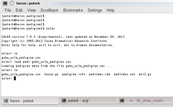
    -3       -2    -1         0   1     2    3

DISC1 rs6675281 polymorphism
               Whole-sample mega-genetic (N=2285)
                            analysis

        N=28             N=390            N=1867
0.15

 0.1

0.05

   0

-0.05
          TT                CT                CC
 -0.1

-0.15

 -0.2

-0.25

 -0.3

-0.35
        Total variance explained in average
        FA values =0.2% (p=0.002)

Downloading solar-eclipse

   We are always in need of few brave
    souls/testers
    • http://www.nitrc.org/projects/se_linux/
    • Stability should improve in the next six month
   Best to contact me to discuss the project
    • pkochunov@gmail.com

Next year’s workshop
   Discussion of new SE features
    • Performance and memory optimization
      strategies
   Voxel-wise, mega-GWAS of fixed effects
    in Enigma-DTI (>5,000 subjects)
   Better multiple comparison corrections
    • Collaboration with Tom Nichols.
   Integration of SE with image analyses
    pipelines
    • Collaborative work with Bennett Landman

Acknowledgements
   Collaborative effort of
    • John Blangero
    • Charles Peters
    • David Glahn
    • Tom Nichols
    • Bennett Landman
    • Neda Jahanshad
    • Paul Thompson
   Supported by EB015611, P01HL045522, R37MH059490,
    R01MH078111, R01MH0708143 and R01MH083824