Molecfit Sabine Moehler - Atmospheric Correction
←
→
Page content transcription
If your browser does not render page correctly, please read the page content below
Atmospheric Correction

                     Molecfit
http://www.eso.org/sci/software/pipelines/skytools/molecfit

                    Sabine Moehler

              Based on a presentation by
                   Wolfgang Kausch
                 (Innsbruck, Austria)

                    Based on a presentation by Wolfgang Kausch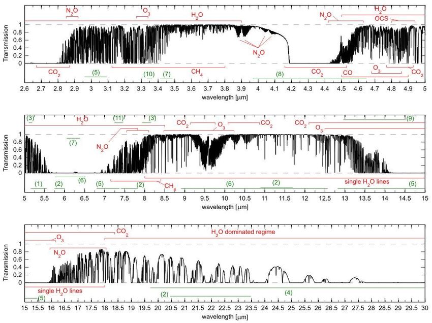
Atmospheric Correction

                    source

                                                              absorption
                        atmosphere
                                                                                emission

                                                  scattering

                                                                                           observer

www.asc-csa.gc.ca                                                                                © Steve Cole

                                     Based on presentation by Wolfgang Kausch
Atmospheric Correction

Atmospheric absorption / optical + NIR

                                                    Smette et al., 2015, A&A 576, A77
       Based on a presentation by Wolfgang Kausch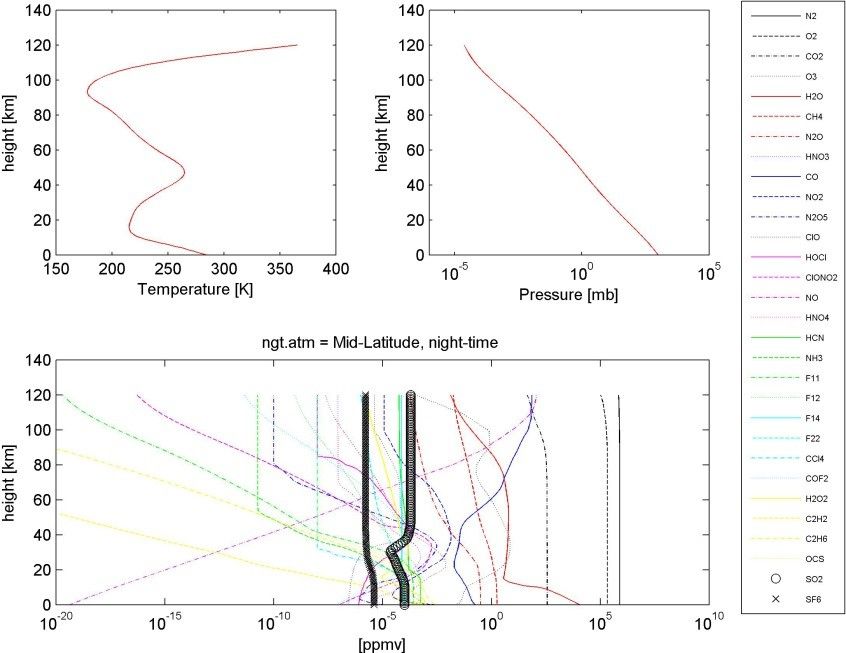
Atmospheric Correction
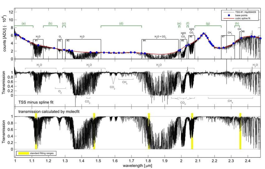
Atmospheric absorption / MIR
Smette et al., 2015, A&A 576, A77
Trace gases: (1) NO, (2) HNO3, (3) COF2, (4) H2O2, (5) HCN, (6) NH3, (7) NO2, (8) N2, (9) C2H2, (10), C2H6, (11) SO2.
Based on a presentation by Wolfgang Kausch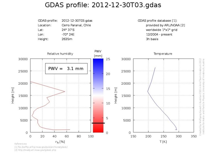
Atmospheric Correction

How can we get rid of this?

         Plan A:
Supplementary calibration
         frames
   „Classical method“

      Based on a presentation by Wolfgang Kausch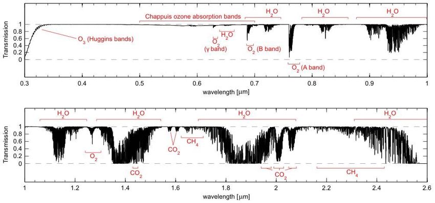
Atmospheric Correction

Required: transmission spectrum

Telluric Standard Stars:

• hot stars without/with few, well known intrinsic spectral features (B-type)
  or solar analogs
• observation in the vicinity, very similar airmass as science target
• observation directly before/after the science target

– expensive in telescope time
– conditions sometimes vary too fast
+ instrument line spread function is the same as for science

                           Based on a presentation by Wolfgang Kausch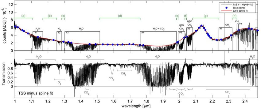
Atmospheric Correction

                                                 Kausch et al, 2015, A&A 576, A78
    Based on a presentation by Wolfgang Kausch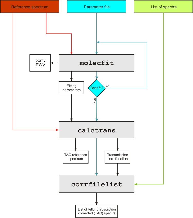
Atmospheric Correction
How can we get rid of this?
Plan :
Modelling
molecfit
Based on a presentation by Wolfgang Kausch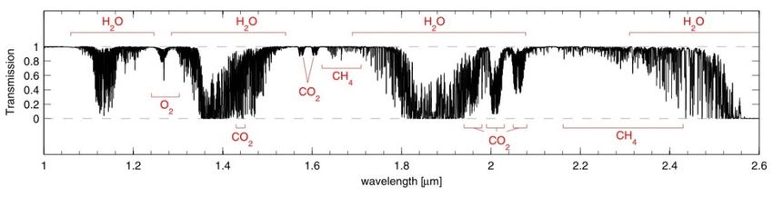
Atmospheric Correction

                Telluric absorption correction with molecfit

 Basic idea ([1],[2]):
 • Derive the atmospheric state from its fingerprint in the science spectra
 • Calculate synthetic transmission spectra corresponding to this state
    by means of a radiative transfer code
 • Fit these spectra iteratively to absorption features in science spectra
 • Use the best-fit transmission for the telluric absorption correction

Features:
• Comprehensive software suite for telluric absorption correction
• Instrument independent
• world-wide use
• based on Ansi-C → high compatibility (Linux+MacOS)
• freely available*

                                                                    [1] Smette et al., 2015, A&A 576, A77
                                                                     [2] Kausch et al, 2015, A&A 576, A78
                                                                   *http://www.eso.org/pipelines/skytools
                           Based on a presentation by Wolfgang Kausch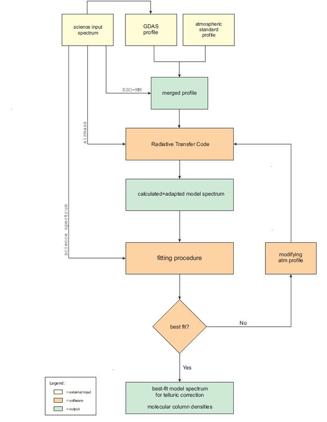
Atmospheric Correction

                                                 fitting of spectral features in the
                                                 fitting ranges → best fit solution

                                                 Calculation of the transmission
                                                 based on the fit + application
                                                 of the telluric abs. correction

                                                 Application of the correction to
                                                 other files.

    Based on a presentation by Wolfgang Kausch
Atmospheric Correction
Radiative transfer code
LBLRTM ([1],[2]):
• Line-By-Line-Radiative-Transfer-Model
• third party code [3]
• V12.2
• widely used in atmospheric research
• still being further developed
• uses LiNeFiLe to retrieve line information from
the High Resolution Transmission database
[1] Clough et al., 2005, J. Quant. Spectrosc. Radiat. Transfer, 91, 233-244
[2] Clough et al., 1992, J. Geophys. Res., 97, 15761-15785
[3] http://rtweb.aer.com/lblrtm_frame.html
Based on a presentation by Wolfgang KauschAtmospheric Correction
Radiative transfer code / line database
HITRAN database([1],[2],[3]):
• 39 different molecules
• 2,713,968 spectral lines
• calculated & observed data
• V13 (HITRAN 2008)
[1] Atomic and Molecular Physics Division, Harvard-Smithsonian Center for Astrophysics
[2] Rothman et al., 2009, Journal of Quantitative Spectroscopy and Radiative Transfer, vol. 110, pp. 533-572
[3] http://www.cfa.harvard.edu/HITRAN/
Based on a presentation by Wolfgang KauschAtmospheric Correction
Radiative transfer code / atmospheric profile
• Static atmospheric standard profile (P, T, mixing ratios for many molecules)
• Global GDAS* weather model: 1° x 1° grid, every 3 h, profiles for P, T, r H
Local meteorological data for height of site: P, T, and rH (taken from FITS header
if present) → ESO MeteoMonitor
atmospheric standard profile
*ftp://ftp.arl.noaa.gov/archives/gdas1/
ppmv = parts per million volume Based on a presentation by Wolfgang KauschAtmospheric Correction molecfit workflow
Based on a presentation by Wolfgang KauschAtmospheric Correction
Fitting procedure
Fitting ranges: lines of intermediate strength; good coverage of
wavelength range; as narrow as possible (better continuum fit and
shorter code run times)
Exclusion regions: no fitting of bad pixels (or other instrumental
defects) and object features
Smette et al., 2015, A&A 576, A77
Based on a presentation by Wolfgang KauschAtmospheric Correction
Fitting procedure
χ2 minimisation by a Levenberg-Marquardt technique (MPFIT [1])
Fitting parameters:
• Scaling factors for molecular profiles
• Coefficients of polynomials for continuum fit Chebyshev polynomials
• Coefficients of Chebyshev polynomials for
modification of wavelength grid
• Widths of boxcar, Gaussian, and Lorentzian
for instrumental profile (alternative: user-
provided kernel → no fit)
● Emissivity of greybody (only for fit of sky
emission spectra in the thermal IR)
[1] Markwardt, C. B. 2009, in Astronomical Society of the Pacific Conference Series,
Vol. 411, Astronomical Data Analysis Software and Systems XVIII, ed.
D. A. Bohlender, D. Durand, & P. Dowler, 251
Based on a presentation by Wolfgang KauschAtmospheric Correction
Invoking molecfit
• GUI: /bin/molecfit_gui
Based on a presentation by Wolfgang KauschAtmospheric Correction
Parameter file: plain ASCII file → text editor
### Driver for MOLECFIT
## DIRECTORY STRUCTURE
# Base directory (default: ".") for the following folder structure:
#
# |--bin/
# |
# |--config/
Sections comments (‚#‘)
# ----|
# |--data/
# |
# |--output/
#
# A relative or an absolute path can be provided. In the former case MOLECFIT
# has to be started in .
basedir: . parameter:
## INPUT DATA
# Data file name (path relative to basedir or absolute path) :
filename: examples/input/crires_spec_jitter_extracted_0000.fits
# ASCII list of files to be corrected for telluric absorption using the
# transmission curve derived from the input reference file (path of list and
- or -
# listed files relative to basedir or absolute path; default: "none")
listname: none
# Type of input spectrum -- 1 = transmission (default); 0 = emission
trans: 1
.
.
.
Based on a presentation by Wolfgang KauschAtmospheric Correction
Parameter file: plain ASCII file → text editor
X-shooter
varkern: 1 (variable kernel, linear increase with wavelength)
columns: NULL FLUX ERRS QUAL (MERGE1D)
columns: WAVE FLUX ERR QUAL (IDP)
H2O O2 (VIS, fit only H2O)
H2O O2 CO CH4 CO2 (NIR fit only H2O)
Based on a presentation by Wolfgang KauschAtmospheric Correction
Parameters: Section „Molecular column“
[…]
# List of molecules to be included in the model
# (default: ’H2O’, N_val: nmolec)
list_molec: H2O CH4 O3
# Fit flags for molecules -- 1 = yes; 0 = no (N_val: nmolec)
fit_molec: 1 1 1
# Values of molecular columns, expressed relatively to the input ATM profile
# columns (N_val: nmolec)
relcol: 1. 1. 1.
[…]
list_molec: List of molecules to be
considered by the radiative
transfer code; Depends on the chosen fitting range
fit only molecules present in spectrum
fit_molec: Defines, whether a molecular column should be fitted or assumed to be constant
relcol: Scaling factor for the molecular column (starting value);
NOTE: # of values in fit_molec and relcol must be equal to number of molecules (order!);
Based on a presentation by Wolfgang KauschAtmospheric Correction
Results / comparison
Comparison with Telluric Standard Star
Object spectrum
molecfit correction
Classical method correction
Kausch et al, 2015, A&A 576, A78
Based on a presentation by Wolfgang KauschAtmospheric Correction
Kausch et al, 2015, A&A 576, A78
Based on a presentation by Wolfgang KauschAtmospheric Correction
Limitations
External:
• Accuracy of the line database
• Radiative transfer code accuracy
• Initial atmospheric profile
Internal:
• No correction for very low T possible
• Low S/N spectra cannot be fitted reliably
• Number of fitting parameters (-fit, continuum, LSF,….)
• Intrinsic spectral features of the object
• Resolution
Kausch et al, 2015, A&A 576, A78
Based on a presentation by Wolfgang KauschAtmospheric Correction
Summary + Outlook
Modelling is a good alternative to supplementary observations
molecfit and skycorr are
• Instrument independent
• world-wide use
• based on Ansi-C → high compatibility
• high flexibility
• freely available*
Will be implemented in future pipelines
*Licenses for outside code to be respected
Based on a presentation by Wolfgang KauschAtmospheric Correction
Molecfit details
● Molecfit User Manual
ftp://ftp.eso.org/pub/dfs/pipelines/skytools/molecfit/VLT-MAN-ESO-19550-5772_Molecfit_User_Manual.pdf
● Molecfit Tutorial
ftp://ftp.eso.org/pub/dfs/pipelines/skytools/molecfit/VLT-MAN-ESO-19550-5928_Molecfit_GUI_and_Tutorial.pdf
Based on a presentation by Wolfgang KauschAtmospheric Correction
Invoking molecfit:
• Reflex
• GUI
• console:
/bin/molecfit
:
contains all information required for the telluric absorption correction for a specific file,
i.e. filenames, fitting parameters, output,….
Based on a presentation by Wolfgang KauschAtmospheric Correction
Parameters: Sections „Directory“ and „Input Data“
[…]
# A relative or an absolute path can be provided. In the former case MOLECFIT
# has to be started in .
basedir: .
## INPUT DATA
# Data file name (path relative to basedir or absolute path)
filename: examples/input/crires_spec_jitter_extracted_0000.fits
# ASCII list of files to be corrected for telluric absorption using the
# transmission curve derived from the input reference file (path of list and
# listed files relative to basedir or absolute path; default: "none")
listname: none
[…]
basedir: In all cases either absolute paths can be given, or paths relative to basedir
filename: File, which is to be corrected. This file is the reference, which is usually used
for fitting and for the correction
listname: ASCII file containing a list of other spectra, which should be corrected with
the same transmission spectrum
Based on a presentation by Wolfgang KauschAtmospheric Correction
Parameters: Sections „Directory“ and „Input Data“
[…]
# Type of input spectrum -- 1 = transmission (default); 0 = emission
trans: 1
# Names of the file columns (table) or extensions (image) containing:
# Wavelength Flux Flux_Err Mask
# - Flux_Err and/or Mask can be avoided by writing ’NULL’
# - ’NULL’ is required for Wavelength if it is given by header keywords
# - parameter list: col_lam, col_flux, col_dflux, and col_mask
columns: Wavelength Extracted_OPT Error_OPT NULL
# Default error relative to mean for the case that the error column is missing
default_error: 0.01
[…]
trans: molecfit can fit both emission and transmission features;
columns: column names of the input file
default_error: If no error column is present one can give a default error here
Based on a presentation by Wolfgang KauschAtmospheric Correction
Parameters: Sections „Directory“ and „Input Data“
[…]
# Multiplicative factor to convert wavelength to micron
# (e.g. nm -> wlgtomicron = 1e-3)
wlgtomicron: 1e-3
# Wavelengths in vacuum (= vac) or air (= air)
vac_air: vac
[…]
wlgtomicron: Molecfit calculates internally in [µm]. Thus one needs to specifiy the
wavelength unit in the input spectrum
vac_air: Wavelength regime; depends on the pipeline output
Based on a presentation by Wolfgang KauschAtmospheric Correction
Parameters: Sections „Directory“ and „Input Data“
[…]
# ASCII or FITS table for wavelength ranges in micron to be fitted
# (path relative to basedir or absolute path; default: "none")
wrange_include: none
# ASCII or FITS table for wavelength ranges in micron to be excluded from the
# fit (path relative to basedir or absolute path; default: "none")
wrange_exclude: none
# ASCII or FITS table for pixel ranges to be excluded from the fit
# (path relative to basedir or absolute path; default: "none")
prange_exclude: examples/config/exclude_crires.dat
[…]
Definition of the range files
wrange_include: Path to the file defining the fitting ranges
wrange_exclude: Exclusion range in space
prange_exclude: Exclusion range in pixel space
Based on a presentation by Wolfgang KauschAtmospheric Correction
Parameters: Section „Results“
[…]
## RESULTS
# Directory for output files (path relative to basedir or absolute path)
output_dir: output
# Name for output files
# (supplemented by "_fit" or "_tac" as well as ".asc", ".atm", ".fits",
# ".par, ".ps", and ".res")
output_name: molecfit_crires
# Plot creation: gnuplot is used to create control plots
# W - screen output only (incorporating wxt terminal in gnuplot)
# X - screen output only (incorporating x11 terminal in gnuplot)
# P - postscript file labelled ’.ps’, stored in
# combinations possible, i.e. WP, WX, XP, WXP (however, keep the order!)
# all other input: no plot creation is performed
plot_creation: XP
# Create plots for individual fit ranges? -- 1 = yes; 0 = no
plot_range: 0
[…]
output_dir: directory where all output files are stored in
output_name: Defines name space for output files
plot_creation: Defines type of output plots
plot_range: Defines whether plots for ALL fitting ranges should be created individually
Based on a presentation by Wolfgang KauschAtmospheric Correction
Parameters: Section „Fit Precision“
[…]
## FIT PRECISION
# Relative chi2 convergence criterion
ftol: 1e-2
# Relative parameter convergence criterion
xtol: 1e-2
[…]
mpfit stops the fitting procedure as soon as either the 2-value or the fitting parameters
change less than a given certain limit
ftol: Convergence criterion for the variation of the 2-value
xtol: Convergence criterion for the variation of the fitting parameters
Note: Use with care!
Based on a presentation by Wolfgang KauschAtmospheric Correction
Parameters: Section „Background and continuum“
[…]
## BACKGROUND AND CONTINUUM
# Conversion of fluxes from phot/(s*m2*mum*as2) (emission spectrum only) to
# flux unit of observed spectrum:
# 0: phot/(s*m^2*mum*as^2) [no conversion]
# 1: W/(m^2*mum*as^2)
# 2: erg/(s*cm^2*A*as^2)
# 3: mJy/as^2
# For other units, the conversion factor has to be considered as constant term
# of the continuum fit.
flux_unit: 0
# Fit of telescope background -- 1 = yes; 0 = no (emission spectrum only)
fit_back: 0
# Initial value for telescope background fit (range: [0,1])
telback: 0.1
[…]
flux_unit: Same as wlgtomicron, but for the flux (internal units: photons/(s*m 2*µm*as2) )
fit_back: Defines, whether the telescope background should be fitted (greybody). Only
important for emission spectra (parameter: trans: 0)
telback: Initial value for the telescope background (greybody factor)
Based on a presentation by Wolfgang KauschAtmospheric Correction
Parameters: Section „Background and continuum“
[…]
# Polynomial fit of continuum --> degree: cont_n
fit_cont: 1
# Degree of coefficients for continuum fit
cont_n: 3
# Initial constant term for continuum fit (valid for all fit ranges)
# (emission spectrum: about 1 for correct flux_unit)
cont_const: 1.
[…]
fit_cont: Defines whether the continuum should be fitted as poynomial
cont_n: degree of continuum polynomial
cont_const: Initial constant continuum value; Can be only roughly in the order of the
continuum level
Based on a presentation by Wolfgang KauschAtmospheric Correction
Parameters: Section „Wavelength solution“
[…]
## WAVELENGTH SOLUTION
# Refinement of wavelength solution using a polynomial of degree wlc_n
fit_wlc: 1
# Polynomial degree of the refined wavelength solution
wlc_n: 3
# Initial constant term for wavelength correction (shift relative to half
# wavelength range)
wlc_const: 0.
[…]
fit_wlc: Defines whether the wavelegth grid should be fitted with a Chebyshev polynome
wlc_n: degree of Chebyshev polynomial
wlc_const: Initial constant term for the wavelength
correctopm
Based on a presentation by Wolfgang KauschAtmospheric Correction Parameters: Section „Resolution“ […] ## RESOLUTION # Fit resolution by boxcar -- 1 = yes; 0 = no fit_res_box: 0 # Initial value for FWHM of boxcar relative to slit width (>= 0. and
Atmospheric Correction
Parameters: Section „Resolution“
[…]

# Fit resolution by Gaussian -- 1 = yes; 0 = no
fit_res_gauss: 1

# Initial value for FWHM of Gaussian in pixels
res_gauss: 1.

# Fit resolution by Lorentzian -- 1 = yes; 0 = no
fit_res_lorentz: 0

# Initial value for FWHM of Lorentzian in pixels
res_lorentz: 0.5

[…]

fit_res_gauss:

rel_gauss: Initial value for FWHM of the GAUSSIAN component

fit_res_lorentz:

res_lorentz: Initial value for FWHM of the LORENTZIAN component

                                       Based on a presentation by Wolfgang Kausch
Atmospheric Correction
Parameters: Section „Instrumental parameters“
[…]
## INSTRUMENTAL PARAMETERS
# Slit width in arcsec (taken from FITS header if present)
slitw: 0.4
slitw_key: ESO INS SLIT1 WID
# Pixel scale in arcsec (taken from this file only)
pixsc: 0.086
pixsc_key: NONE
[…]
slitw: Slit width in arcsec (taken from FITS header if present)
slitw_key: fitsheader keyword describing the slit width
pixsc: Pixel scale in arcsec
pixsc_key: fitsheader keyword describing the pixel scale
Based on a presentation by Wolfgang KauschAtmospheric Correction
Parameters: Sections „Ambient parameters“ and „Atmospheric
profiles“
These sections incorporate parameters describing the date/time of the observations, the
airmass, atmopsheric state during the time of the observations (r H, P, T, M1 temperature,…),
longitude/latitude of observatory, ….
Mostly taken from fits header keyword („_key“), or should not be modified.
Based on a presentation by Wolfgang KauschYou can also read