Sparse Semantic Segmentation Network - (AF)2-S3Net: Attentive Feature Fusion with Adaptive Feature Selection for

(AF)2 -S3Net: Attentive Feature Fusion with Adaptive Feature Selection for
 Sparse Semantic Segmentation Network

 Ran Cheng1 , Ryan Razani1 , Ehsan Taghavi1 , Enxu Li1 , and Bingbing Liu1
 1
 Noah Ark’s Lab, Huawei, Markham, ON, Canada
arXiv:2102.04530v1 [cs.CV] 8 Feb 2021

 Abstract
 Autonomous robotic systems and self driving cars rely
 on accurate perception of their surroundings as the safety
 of the passengers and pedestrians is the top priority. Se-
 mantic segmentation is one of the essential components of
 road scene perception that provides semantic information
 of the surrounding environment. Recently, several meth- SalsaNext MinkNet42
 ods have been introduced for 3D LiDAR semantic segmen-
 tation. While they can lead to improved performance, they
 are either afflicted by high computational complexity, there-
 fore are inefficient, or they lack fine details of smaller in-
 stances. To alleviate these problems, we propose (AF)2 -
 S3Net, an end-to-end encoder-decoder CNN network for 3D
 LiDAR semantic segmentation. We present a novel multi-
 branch attentive feature fusion module in the encoder and Ours Ground Truth
 a unique adaptive feature selection module with feature
 map re-weighting in the decoder. Our (AF)2 -S3Net fuses Figure 1: Comparison of our proposed method with Sal-
 the voxel-based learning and point-based learning meth- saNext [9] and MinkNet42 [8] on SemanticKITTI bench-
 ods into a unified framework to effectively process the large mark [3].
 3D scene. Our experimental results show that the proposed
 method outperforms the state-of-the-art approaches on the Although image semantic segmentation is an important
 large-scale SemanticKITTI benchmark, ranking 1st on the step in realizing self driving cars, the limitations of a vision
 competitive public leaderboard competition upon publica- sensor such as inability to record data in poor lighting con-
 tion. ditions, variable sensor sensitivity, lack of depth informa-
 tion and limited field-of-view (FOV) makes it difficult for
 vision sensors to be the sole primary source for scene un-
 1. Introduction derstanding and semantic segmentation. In contrast, Light
 Understanding of the surrounding environment has been Detection and Ranging (LiDAR) sensors can record accu-
 one of the most fundamental tasks in autonomous robotic rate depth information regardless of the lighting conditions
 systems. With the challenges introduced with recent tech- with high density and frame rate, making it a reliable source
 nologies such as self-driving cars, a detailed and accurate of information for critical tasks such as self driving.
 understanding of the road scene has become a main part LiDAR sensor generates point cloud by scanning the
 of any outdoor autonomous robotic system in the past few environment and calculating time-of-flight for the emitted
 years. To achieve an acceptable level of road scene under- laser beams. In doing so, LiDARs can collect valuable in-
 standing, many frameworks benefit from image semantic formation, such as range (e.g., in Cartesian coordinates) and
 segmentation, where a specific class is predicted for every intensity (a measure of reflection from the surface of the ob-
 pixel in the input image, giving a clear perspective of the jects). Recent advancement in LiDAR technology makes it
 scene. possible to generate high quality, low noise and dense scans

 1

from desired environments, making the task of scene un- (FCNN) and a Conditional Random Fields (CRF) as a Re-
derstanding a possibility using LiDARs. Although rich in current Neural Network (RNN) layer. In order to reduce
information, LiDAR data often comes in an unstructured number of the parameters in the network, SqueezeSeg in-
format and partially sparse at far ranges. These characteris- corporates “fireModules” from [14]. In a subsequent work,
tics make the task of scene understating challenging using SqueezeSegV2 [32] introduced Context Aggregation Mod-
LiDAR as primary sensor. Nevertheless, research in scene ule (CAM), a refined loss function and batch normalization
understanding and in specific, semantic segmentation using to further improve the model. SqueezeSegV3 [34] stands
LiDARs, has seen an increase in the past few years with the on the shoulder of [31, 14], adopting a Spatially-Adaptive
availability of datasets such as semanticKITTI [3]. Convolution (SAC) to use different filters in different loca-
 The unstructured nature and partial sparsity of LiDAR tions in relation to the input image. Inspired by YOLOv3
data brings challenges to semantic segmentation. However, [25], RangeNet++ [21] uses a DarkNet backbone to process
a great effort has been put by researchers to address these a range-image. In addition to a novel CNN, RangeNet++
obstacles and many successful methods have been proposed [21] proposes an efficient way of predicting labels for the
in the literature (see Section 2). From real-time methods full point cloud using a fast implementation of K-nearest
which use projection techniques to benefit from the avail- neighbour (KNN).
able 2D computer vision techniques, to fully 3D approaches Benefiting from a new 2D projection, PolarNet [37]
which target higher accuracy, there exist a range of methods takes on a different approach using a polar Birds-Eye-View
to build on. To better process LiDAR point cloud in 3D and (BEV) instead of the standard 2D grid-based BEV projec-
to overcome limitations such as non-uniform point densi- tions. Moreover, PolarNet encapsulates the information
ties and loss of granular information in voxelization step, regarding each polar gird using PointNet, rather than us-
we propose (AF)2 -S3Net, which is built upon Minkowski ing hand crafted features, resulting in a data-driven feature
Engine [8] to suit varying levels of sparsity in LiDAR point extraction, a nearest-neighbor-free method and a balanced
clouds, achieving state-of-the-art accuracy in semantic seg- grid distribution. Finally, in a more successful attempt, Sal-
mentation methods on SemanticKITTI [3]. Fig. 1 demon- saNext [9], makes a series of improvements to the backbone
strates qualitative results of our approach compared to Sal- introduced in SalsaNet [1] such as, a new global contextual
saNext [9] and MinkNet42 [8]. We summarize our contri- block, an improved encoder-decoder and Lovász-Softmax
butions as, loss [4] to achieve state-of-the-art results in 2D LiDAR se-
 mantic segmentation using range-image input.
 • An end-to-end encoder-decoder 3D sparse CNN that
 achieves state-of-the-art accuracy in semanticKITTI 2.2. 3D semantic Segmentation
 benchmark [3];
 The category of large scale 3D perception methods
 • A multi-branch attentive feature fusion module in the kicked off by early works such as [6, 20, 23, 29, 39]
 encoder to learn both global contexts and local details; in which a voxel representation was adopted to capital-
 • An adaptive feature selection module with feature map ize vanilla 3D convolutions. In attempt to process un-
 re-weighting in the decoder to actively emphasize the structured point cloud directly, PointNet [22] proposed a
 contextual information from feature fusion module to Multi-Layer Perception (MLP) to extract features from in-
 improve the generalizability; put points without any voxelization. PointNet++ [24] which
 is an extension to the nominal work Pointnet [22], intro-
 • A comprehensive analysis on semantic segmenta- duced sampling at different scales to extract relevant fea-
 tion and classification performance of our model tures, both local and global. Although effective for smaller
 as opposed to existing methods on three bench- point clouds, Methods rely on Pointnet [22] and its varia-
 marks, semanticKITTI [3], nuScenes-lidarseg [5], and tions are slow in processing large-scale data.
 ModelNet40 [33] through ablation studies, qualitative Down-sampling is at the core of the method proposed
 and quantitative results. in RandLA-Net [13]. As down-sampling removes features
 randomly, a local feature aggregation module is also intro-
2. Related Work duced to progressively increase the receptive field for each
 3D point. The two techniques used jointly to achieve both
2.1. 2D semantic Segmentation
 efficiency and accuracy in large-scale point cloud seman-
 SqueezeSeg [31] is one of the first works on LiDAR tic segmentation. In a different approach, Cylinder3D [38]
semantic segmentation using range-image, where LiDAR uses cylindrical grids to partition the raw point cloud. To
point cloud projected on a 2D plane using spherical trans- extract features, authors in [38] introduced two new CNN
formation. SqueezeSeg [31] network is based on an blocks. An asymmetric residual block to ensure features re-
encoder-decoder using Fully Connected Neural Network lated to cuboid objects are being preserved and Dimension-

decomposition based Context Modeling in which multiple to achieve good performance on a large-scale driving scene
low-rank contexts are merged to model a high-ranked tensor covering more than 100m with non-uniform point densi-
suitable for 3D point cloud data. ties. Majority of the LiDAR segmentation methods attempt
 Authors in KPConv [28] introduced a new point convo- to either transform 3D LiDAR point cloud into 2D image
lution without any intermediate steps taken in processing using spherical projection (i.e., perspective, bird-eye-view)
point clouds. In essence, KPConv is a convolution operation or directly process the raw point clouds. The former ap-
which takes points in the neighborhood as input and pro- proach abandons valuable 3D geometric structures and suf-
cesses them with spatially located weights. Furthermore, a fers from information loss due to projection process. The
deformable version of this convolution operator was also in- latter approach requires heavy computations and not feasi-
troduced that learns local shifts to make them adapt to point ble to be deployed in constrained systems with limited re-
cloud geometry. Finally, MinkowskiNet [8] introduces a sources. Recently, sparse 3D convolution became popular
novel 4D sparse convolution for spatio-temporal 3D point due to its success on outdoor LiDAR semantic segmentation
cloud data along with an open-source library to support task. However, out of a few methods proposed in [8, 27], no
auto-differentiation for sparse tensors. Overall, where we advanced feature extractors were proposed to enhance the
consider the accuracy and efficiency, voxel-based methods results similar to computer vision and 2D convolutions.
such as MinkowskiNet [8] stands above others, achieving To overcome this, we propose (AF)2 -S3Net for Li-
state-of-the-art results within all sub-categories of 3D se- DAR semantic segmentation in which a baseline model of
mantic segmentation. MinkNet42 [8] is transformed into an end-to-end encoder-
 decoder with attention blocks and achieves stat-of-the-art
2.3. Hybrid Methods results. In this Section we first present the proposed net-
 Hybrid methods, where a mixture of voxel-based, work architecture along with its novel components, namely
projection-based and/or point-wise operations are used to AF2M and AFSM. Then, the network optimization is intro-
process the point cloud, has been less investigated in the duced followed by the training details.
past, but with availability of more memory efficient designs,
are becoming more successful in producing competitive re- 3.1. Problem statement
sults. For example, FusionNet [35] uses a voxel-based MLP, Lets consider a semantic segmentation task in which a
called voxel-based mini-PointNet which directly aggregates LiDAR point cloud frame is given with a set of unordered
features from all the points in the neighborhood voxels to points (P, L) = ({pi , li }) with pi ∈ Rdin and i = 1, ..., N ,
the target voxel. This allows FusionNet [35] to search where N denotes the number of points in an input point
neighborhoods with low complexity, processing large scale cloud scan. Each point pi contains din input features, i.e.,
point cloud with acceptable performance. In another ap- Cartesian coordinates (x, y, z), intensity of returning laser
proach, 3D-MiniNet [2] proposes a learning-based projec- beam (i), colors (R, G, B), etc. Here, li ∈ R represents the
tion module to extract local and global information from the ground truth labels corresponding to each point pi . How-
3D data and then feeds it to a 2D FCNN in order to gener- ever, in object classification task, a single class label L is
ate semantic segmentation predictions. In a slightly differ- assigned to an individual scene containing P points.
ent approach, MVLidarNet [7] benefits form range-image Our goal is to learn a function Fcls (., Φ) parameterized
LiDAR semantic segmentation to refine object instances in by Φ that assigns a single class label L for all the points in
bird’s-eye-view perspective, showcasing the applicability of the point cloud or in other words, Fseg (., Φ), that assigns a
LiDAR semantic segmentation in real-world applications. per point label ĉi to each point pi . To this end, we propose
 Finally, SPVNAS [27] builds upon the Minkowski En- (AF)2 -S3Net to minimize the difference between the pre-
gine [8] and designs a hybrid approach of using 4D sparse dicted label(s), L̂ and ĉi , and the ground truth class label(s),
convolution and point-wise operations to achieve state-of- L and li , for the tasks of classification and segmentation,
the-art results in LiDAR semantic segmentation. To do this, respectively.
authors in SPVNAS [27] use a neural architecture search
(NAS) [18] to efficiently design a NN, based on their novel 3.2. Network architecture
Sparse Point-Voxel Convolution (SPVConv) operation.
 The block diagram of the proposed method, (AF)2 -
3. Proposed Approach S3Net, is illustrated in Fig. 2. (AF)2 -S3Net consists of
 a residual network based backbone and two novel mod-
 The sparsity of outdoor-scene point clouds makes it diffi- ules, namely Attentive Feature Fusion module (AF2M) and
cult to extract spatial information compared to indoor-scene Adaptive Feature Selection Module (AFSM). The model
point clouds with fixed number of points or based on the takes in a 3D LiDAR point cloud and transforms it into
dense image-based dataset. Therefore, it is difficult to lever- sparse tensors containing coordinates and features corre-
age the indoor-scene or image-based segmentation methods sponding to each point. Then, the input sparse tensor is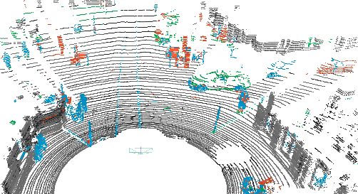

Attentive Feature Fusion Adaptive Feature Selection
 α Conv
 Conv Conv Conv 1 1 (2x2x2)
 (3x3x3) (5x5x5) (8x8x8)
 [32, 32]
 × 2 [32, 32]
 [4, 64] [64, 32] 3 �
 ′1
 [N, 32] [N, 32]
 β
 Conv Conv ℎ1 2 Conv
 Conv J
 (4x4x4)
 [4, 64]
 (4x4x4)
 [64, 32]
 × � (2x2x2) (2x2x2)
 [32, 32]
 ℎ2 [32, 32] ′2 Sparse Global
 [ , ]
 Conv
 [N, 32]
 γ F [N, 32]
 � Pooling
 Sparse Linear
 Excitation ×
 ℎ3 3 [N, 96] Squeeze θ
 [3, 96]
 (12x12x12)
 [4, 32]
 × Conv
 (2x2x2) �
 [N, 32] [32, 32] (1- θ)
 Broadcast
 ℎ : Conv (2x2x2)[32, 1] [N, 32]
 � ′3
 
 π : Conv (2x2x2)[3, 32] (∗,∗,∗)= 
 = 1 , , = π : Concatenation (∗,∗,∗) = 1 , 2 , 3 : Concatenation

 Adaptive Feature
 Selection
 Input 3D Point Cloud Output 3D Point Cloud
 1 2 3
 c
 J Conv Conv Conv TrConv TrConv TrConv TrConv Conv
 Attentive Feature
 (3x3x3) (3x3x3) (3x3x3) (3x3x3) (3x3x3) (3x3x3) (3x3x3) (3x3x3)
 Fusion
 [32, 64] [64, 128] [128, 256] [256, 128] [128, 64] [64, 96] [192, 32] [32, 20]
 [ , ] [ , ]

 3D Coordinates Point Features c : Concatenation × : Multiplication �
 : Sum Point label

Figure 2: Overview of (AF)2 -S3Net. The top left block is Attentive Feature Fusion Module (AF2M) that aggregates Lo-
cal and global context using a weighted combination of mutually exclusive learnable masks, α, β, and γ. The top right
block illustrates how Adaptive Feature Selection Module (AFSM) uses shared parameters to learn inter relationship between
channels across multi-scale feature maps from AF2M. (best viewed on display)

processed by (AF)2 -S3Net which is built upon 3D sparse lize the attention layers hi (·), ∀i ∈ {1, 2, 3}, by adding the
convolution operations which suits sparse point clouds and residual damping factor. This damping factor is the output
effectively predicts a class label for each point given a Li- of residual convolution layer π. Further, function π can be
DAR scan. formulated as
 A sparse tensor can be expressed as Ps = [C, F ], where
C ∈ RN ×M represents the input coordinate matrix with π , sigmoid(bn(conv(fenc (·)))) (2)
M coordinates and F ∈ RN ×K denotes its correspond- Finally, the output of AF2M is generated by F(g(·)), where
ing feature matrix with K feature dimensions. In this F is used to align the sparse tensor scale space with the
work, we consider 3D coordinates of points (x, y, z), as our next convolution block. As illustrated in Fig. 2 (top-left),
sparse tensor coordinate C, and per point normal features for each hi , ∀i ∈ {1, 2, 3}, the corresponding gradient of
(nx , ny , nz ) along with intensity of returning laser beam (i) weight whi can be computed as:
as our sparse tensor feature F . Exploiting normal features
helps the model to learn additional directional information, ∂J ∂g ∂fenc ∂J ∂g ∂π
 whi = whi − − (3)
hence, the model performance can be improved by differen- ∂g ∂fenc ∂hi ∂g ∂π ∂hi
tiating the fine details of the objects. The detailed descrip- where J is the output of F. Considering g(·) is a linear
tion of the network architecture is provided below. function of concatenated features x̄ and ∆, we can rewrite
 Attentive Feature Fusion (AF2M): To better extract the Eq. 3 as follows:
global contexts, AF2M embodies a hybrid approach, cover-
ing small, medium and large kernel sizes, which focuses ∂J ∂fenc ∂J ∂π
 whi = whi − x̄ − (4)
on point-based, medium-scale voxel-based and large-scale ∂g ∂hi ∂g ∂hi
voxel-based features, respectively. The block diagram of where ∂f∂henc = Sj (δij − Sj ) is the Jacobian of softmax
AF2M is depicted in Fig. 2 (top-left). Principally, the pro- i
 function S(x̄) : RN → RN and maps ith input feature
posed AF2M fuses the features x̄ = [x1 , x2 , x3 ] at the cor-
 column to jth output feature column, and δ is Kronecker
responding branches using g(·) which is defined as,
 delta function where δi=j = 1 and δi6=j = 0. As shown in
 g(x1 , x2 , x3 ) , αx1 + βx2 + γx3 + ∆ (1) Eq. 5,

where α, β and γ are the corresponding coefficients that
 −S12
  
 S1 (1 − S2 ) ...
scale the feature columns for each point in the sparse tensor,
 Sj (δij − Sj ) =  .. ..  (5)
  
and are processed by function fenc (·) as shown in Fig. 2. . .
Moreover, the attention residuals, ∆, is introduced to stabi- 2
 SN (1 − S1 ) ... −SN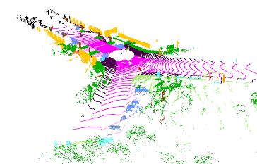

when the softmax output S is close to 0, the term ∂f∂henc i
 branches to the last decoder block, ensures that the error
 approaches to zero which prompts no gradient, and when S gradient propagates back to the encoder branches for better
 is close to 1, the gradient is close to identity matrix. As a learning stability.
 result, when S → 1, all values in α or β or γ get very high
 confidence and the update of whi becomes: 3.3. Network Optimization
 We leveraged a linear combination of geo-aware
 ∂J ∂π ∂J
 whi = whi − + x̄I (6) anisotrophic [17], Exponential-log loss [30] and Lovász
 ∂g ∂hi ∂g loss [4] to optimize our network. In particular, geo-aware
 and in the case of S → 0, the update gradient will only anisotrophic loss is beneficial to recover the fine details in
 depends on π. Fig. 3 further illustrates the capability of the a LiDAR scene. Moreover, Exponential-log loss [30] loss
 proposed AF2M and highlights the effect of each branch is used to further improve the segmentation performance by
 visually. focusing on both small and large structures given a highly
 unbalanced dataset.
 J
 The geo-aware anisotrophic loss can be computed by,
 J = F[32, 32] α 1 + β 2 + γ 3 + ∆ Attentive
 voting
 α 1 Feature Fusion
 β 2
 +∆
 γ 3 C
 1 X X MLGA
 Lgeo (y, ŷ) = −
 N ψ
 yijk,c log ŷijk,c (7)
 [ ×1] [ ×3] [ ×32]
 c=1
 i,j,k

 where y and ŷ are the ground truth label and predicted la-
 bel. Parameter N is the local tensor neighborhood and
 in our experiment, we empirically set it as 5 (a 10 voxels
 PΨ cube). Parameter C is the semantic classes, MLGA =
 size
 Sparse ψ=1 (cp ⊕ cqψ ), defined in [17]. We normalized local ge-
 ometric anisotropy within the sliding window Ψ of the cur-
 Dense rent voxel cell p and its neighbor voxel grid qψ ∈ Ψ.
 Vegetation Side walk Road
 Therefore, the total loss used to train the proposed net-
 Unlabeled F Conv (2x2x2)
 Person Traffic-sign Pole Trunk ∆ Attention Residual work is given by,

Figure X: Illustration
 Figure of Attentive Feature
 3: Illustration Fusion andFeature
 of Attentive spatial geometry
 Fusion of point
 and cloud.
 spa- Ltot (y, ŷ) = w1 Lexp (y, ŷ) + w2 Lgeo (y, ŷ) + w3 Llov (y, ŷ)
The three labels $\alpha x_{1}$, $\beta x_{2}$, and $\gamma x_{3}$ represent the
 tial geometry
branches of point
 in AF2M encoder block. cloud. The three
 The first branch, x_{1}$,αx
 labels
 $\alpha 1 , βx
 learns 2 , and
 to capture
 (8)
and γx
 emphasize the fine details
 3 represent for smaller instances
 the branches in AF2M such as person, pole
 encoder and traffic-
 block. The
sign across the driving scenes with varying point densities. The shallower branches, where w1 , w2 , and w3 denote the weights of Exponential-
 first branch, αx , learns to capture and emphasize
$\beta x_{2}$ and $\gamma x_{3}$, learn different attention-maps that focus on
 1 the fine
 details
global for
 contexts smaller
 embodied instances
 in larger such
 instances such as person, pole
 as vegetation, and
 sidewalk andtraffic-
 road
 log loss [30], geo-aware anisotrophic, and Lovász loss, re-
surface
 sign across the driving scenes with varying point densi- spectively. They are set as 1, 1.5 and 1.5 in our experiments.
 ties. The shallower branches, βx2 and γx3 , learn different
 attention-maps that focus on global contexts embodied in 4. Experimental results
 larger instances such as vegetation, sidewalk and road sur- We base our experimental results on three dif-
 face. (best viewed on display) ferent dataset, namely, SemanticKITTI, nuScenes and
 Adaptive Feature Selection module (AFSM): The ModelNet40 to show the applicability of the proposed
 block diagram of AFSM is shown in Fig. 2 (top-right). methods in different scenes and domains. As for the Se-
 In AFSM decoder block, the feature maps from multiple manticKITTI and ModelNet40, (AF)2 -S3Net is compared
 branches in AF2M, x1 , x2 , and x3 , are further processed to the previous state-of-the-art, but due to a recently an-
 0 0
 by residual convolution units. The resulted output, x1 , x2 , nounce challenge for nuScenes-lidarseg dataset [5], we pro-
 0
 and x3 , are concatenated, shown as fdec , and are passed vide our own evaluation results against the baseline model.
 into a shared squeeze re-weighting network [12] in which To evaluate the performance of the proposed method
 different feature maps are voted. This module acts like an and compare with others, we leverage mean Intersection
 adaptive dropout that intentionally filters out several feature over Union (mIoU) as our evaluation metric. mIoU
 maps that are not contributing to the final results. Instead is the most popular metric for evaluating semantic point
 of directly passing through the weighted feature maps as cloud
 Pn segmentation and can be formalized as mIoU =
 1 T Pc
 output, we employed a damping factor θ = 0.35, to regu- n c=1 T Pc +F Pc +F Nc , where T Pc is the number of true
 larize the weighting effect. It is worth noting that the skip positive points for class c, F Pc is the number of false posi-
 connection connecting the attentive feature fusion module tives, and F Nc is the number of false negatives.

SemanticKITTI

 car car car

 SalsaNext MinkNet42 Ours Ground Truth
NuScenes

 motorcycle
 motorcycle motorcycle

 SalsaNext MinkNet42 Ours Ground Truth

Figure 4: Compared to SalsaNext and MinkNet42, our method has a lower error (shown in red) recognizing region surface
and smaller objects on nuScenes validation set, thanks to the proposed attention modules.

 As for the training parameters, we trained our model beled data to advance self driving car technology. Among
with SGD optimizer with momentum of 0.9 and learning these 1000 scenes, 850 of them is reserved for training and
rate of 0.001, weight decay of 0.0005 for 50 epochs. The validation, and the remaining 150 scenes for testing. The
experiments are conducted using 8 Nvidia V100 GPUs. labels are, to some extent, similar to the semanticKITTI
 dataset [3], making it a new challenge to propose methods
4.1. Quantitative Evaluation that can handle both datasets well, given the different sen-
 sor setups and environment they record the dataset. In Ta-
 In this Section, we provide quantitative evaluation of ble 2, we compared our proposed method with MinkNet42
(AF)2 -S3Net on two outdoor large-scale public dataset: [8] baseline and the projection based method SalsaNext [9].
SemanticKITTI [3] and nuScenes-lidarseg dataset [5] for Results in Table 2 shows that our proposed method can han-
semantic segmentation task and on ModelNet40 [33] for dle the small objects in nuScenes dataset and indicates a
classification task. large margin improvement from the competing methods.
SemanticKITTI dataset: we conduct our experiments Considering the large difference between the two public
on SemanticKITTI [3] dataset, the largest dataset for au- datasets, we can prove that our work can generalize well.
tonomous vehicle LiDAR segmentation. This dataset is
based on the KITTI dataset introduced in [11], containing
41000 total frames which captured in 21 sequences. We list ModelNet40: to expand and evaluate the capabilities of the
our experiments with all other published works in Table 1. proposed method in different applications, ModelNet40, a
As shown in Table 1, our method achieves state-of-the-art 3D object classification dataset [33] is adopted for evalu-
performance in SemanticKITTI test set in terms of mean ation. ModelNet40 contains 12, 311 meshed CAD models
IoU. With our proposed method, (AF)2 -S3Net, we see a from 40 different object categories. From all the samples,
2.7% improvement from the second best method [27] and 9, 843 models are used for training and 2, 468 models for
15.4% improvement from baseline model (MinkNet42 [8]). testing. To evaluate our method against existing stat-of-the-
Our method dominates greatly in classifying small objects art, we compare (AF)2 -S3Net with techniques in which a
such as bicycle, person and motorcycle, making it a reli- single input (e.g., single view, sampled point cloud, voxel)
able solution to understating complex scenes. It is worth has been used to train and evaluate the models. To make
noting that (AF)2 -S3Net only uses the voxelized data as (AF)2 -S3Net compatible for the task of classification, the
input, whereas the competing methods like SPVNAS [27] decoder part of the network is removed and the output of the
use both voxelized data and point-wise features. encoder is directly reshaped to the number of the classes in
Nuscenes dataset: to prove the generalizability of our ModelNet40 dataset. Moreover, the model is trained only
proposed method, we trained our network with nuScenes- using cross-entropy loss. Table 3 presents the overall classi-
lidarseg dataset [5], one of the recently available large-scale fication accuracy results for our proposed method and pre-
datasets that provides point level labels of LiDAR point vious state-of-the-art. With the introduction of AF2M in
clouds. It consists of 1000 driving scenes from various lo- our network, we achieved similar performance to the point-
cations in Boston and Singapore, providing a rich set of la- based methods which leverage fine-grain local features.

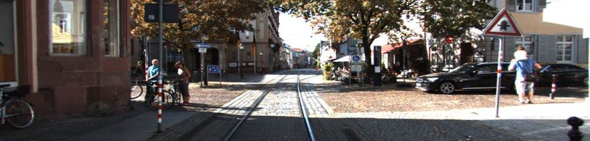
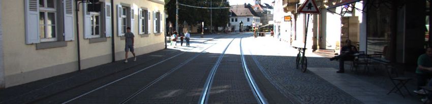
Other-vehicle

 Other-ground
 Motorcyclist

 Traffic-sign
 Motorcycle

 Vegetation
 Mean IoU

 Sidewalk
 Bicyclist

 Building
 Parking
 Bicycle

 Terrain
 Person

 Trunk
 Fence
 Truck

 Road

 Pole
 Car
 Method
 S-BKI [10] 51.3 83.8 30.6 43.0 26.0 19.6 8.5 3.4 0.0 92.6 65.3 77.4 30.1 89.7 63.7 83.4 64.3 67.4 58.6 67.1
 RangeNet++ [21] 52.2 91.4 25.7 34.4 25.7 23.0 38.3 38.8 4.8 91.8 65.0 75.2 27.8 87.4 58.6 80.5 55.1 64.6 47.9 55.9
 LatticeNet [26] 52.9 92.9 16.6 22.2 26.6 21.4 35.6 43.0 46.0 90.0 59.4 74.1 22.0 88.2 58.8 81.7 63.6 63.1 51.9 48.4
 RandLA-Net [13] 53.9 94.2 26.0 25.8 40.1 38.9 49.2 48.2 7.2 90.7 60.3 73.7 20.4 86.9 56.3 81.4 61.3 66.8 49.2 47.7
 PolarNet [37] 54.3 93.8 40.3 30.1 22.9 28.5 43.2 40.2 5.6 90.8 61.7 74.4 21.7 90.0 61.3 84.0 65.5 67.8 51.8 57.5
 MinkNet42 [8] 54.3 94.3 23.1 26.2 26.1 36.7 43.1 36.4 7.9 91.1 63.8 69.7 29.3 92.7 57.1 83.7 68.4 64.7 57.3 60.1
 3D-MiniNet [2] 55.8 90.5 42.3 42.1 28.5 29.4 47.8 44.1 14.5 91.6 64.2 74.5 25.4 89.4 60.8 82.8 60.8 66.7 48.0 56.6
 SqueezeSegV3 [34] 55.9 92.5 38.7 36.5 29.6 33.0 45.6 46.2 20.1 91.7 63.4 74.8 26.4 89.0 59.4 82.0 58.7 65.4 49.6 58.9
 Kpconv [28] 58.8 96.0 30.2 42.5 33.4 44.3 61.5 61.6 11.8 88.8 61.3 72.7 31.6 90.5 64.2 84.8 69.2 69.1 56.4 47.4
 SalsaNext [9] 59.5 91.9 48.3 38.6 38.9 31.9 60.2 59.0 19.4 91.7 63.7 75.8 29.1 90.2 64.2 81.8 63.6 66.5 54.3 62.1
 FusionNet [35] 61.3 95.3 47.5 37.7 41.8 34.5 59.5 56.8 11.9 91.8 68.8 77.1 30.8 92.5 69.4 84.5 69.8 68.5 60.4 66.5
 KPRNet [15] 63.1 95.5 54.1 47.9 23.6 42.6 65.9 65.0 16.5 93.2 73.9 80.6 30.2 91.7 68.4 85.7 69.8 71.2 58.7 64.1
 SPVNAS [27] 67.0 97.2 50.6 50.4 56.6 58.0 67.4 67.1 50.3 90.2 67.6 75.4 21.8 91.6 66.9 86.1 73.4 71.0 64.3 67.3
 (AF)2-S3Net [Ours] 69.7 94.5 65.4 86.8 39.2 41.1 80.7 80.4 74.3 91.3 68.8 72.5 53.5 87.9 63.2 70.2 68.5 53.7 61.5 71.0

 Table 1: Segmentation IoU (%) results on the SemanticKITTI [3] test dataset.
 Construction

 Traffic cone
 Motorcycle

 flat ground
 Mean IoU

 Vegetation
 Pedestrian
 FW mIoU

 Manmade
 Driveable

 Sidewalk
 Bicycle

 surface
 vehicle

 Terrain
 Barrier

 Trailer

 Truck

 Other
 Bus

 Car

 Method
 SalsaNext [9] 82.8 58.8 56.6 4.7 77.1 81.0 18.4 47.5 52.8 43.5 38.3 65.7 94.2 60.0 68.9 70.3 81.2 80.5
 MinkNet42 [8] 82.7 60.8 63.1 8.3 77.4 77.1 23.0 55.1 55.6 50.0 42.5 62.2 94.0 67.2 64.1 68.6 83.7 80.8
 (AF)2 -S3Net [Ours] 83.0 62.2 60.3 12.6 82.3 80.0 20.1 62.0 59.0 49.0 42.2 67.4 94.2 68.0 64.1 68.6 82.9 82.4

Table 2: Segmentation IoU (%) results on the nuScenes-lidarseg [5] validation dataset. Frequency-Weighted IoU denotes that
each IoU is weighted by the point-level frequency of its class.

 fine details in a scene. To demonstrate this, we train (AF)2 -
 S3Net on SemanticKITTI as explained above and visualize
 a test frame. In Fig. 5 we highlight the points with top 5%
 feature norm from each scaled feature maps of αx1 , βx2
 and γx3 with cyan, orange and green colors, respectively.
 It can be observed that our model learns to put its attention
 on small instances (i.e., person, pole, bicycle, etc.) as well
 as larger instances (i.e., car, region boundaries, etc.). Fig. 4
 shows some qualitative results on SemanticKITTI (top) and
 Attention Map Prediction nuScenes (bottom) benchmark. It can be observed that the
 proposed method surpasses the baseline (MinkNet42 [8])
Figure 5: Reference image (top), Prediction (bottom-right), and range-based SalsaNext [9] by a large margin, which
attention map (bottom-left) on SemanticKITTI test set. failed to capture fine details such as cars and vegetation.
Color codes are: road | side-walk | parking | car |
bicyclist | pole | vegetation | terrain | trunk | building 4.3. Ablation Studies
| other-structure | other-object.
 To show the effectiveness of the proposed attention
4.2. Qualitative Evaluation mechanisms, namely, AF2M and AFSM introduced in Sec-
 tion 3, along with other design choices such as loss func-
 In this section, we visualize the attention maps in AF2M tions, this section is dedicated to a thorough ablation study
by projecting the scaled feature maps back to original point starting from our baseline model introduced in [8]. The
cloud. Moreover, to better present the the improvements baseline is MinkNet42 which is a semantic segmentation
that has been made against the baseline model MinkNet42 residual NN model for 3D sparse data. To start off with a
[8] and SalsaNext [9], we provide the error maps which well trained baseline, we use Exponential Logarithmic Loss
highlights the superior performance of our method. [30] to train the model which results in 59.8% mIoU accu-
 As shown in Fig. 5, our method is capable of capturing racy for the validation set on semanticKITTI.

Method Input Main operator Overall Accuracy (%)
 Vox-Net [20] voxels 3D Operation 83.00
 Mink-ResNet50 [8] voxels Sparse 3D Operation 85.30
 Pointnet [22] point cloud Point-wise MLP 89.20
 Pointnet++ [24] point cloud Local feature 90.70
 DGCNN[36] (1 vote) point cloud Local feature 91.84
 GGM-Net [16] point cloud Local feature 92.60
 RS-CNN [19] point cloud Local feature 93.60
 Ours (AF2M) voxels Sparse 3D Operation 93.16

 Table 3: Classification accuracy results on ModelNet40 dataset [33], for input size 1024 × 3.

 Next, we add our proposed AF2M to the baseline model and SalsaNext w.r.t. the distance to the ego-vehicle’s Li-
to help the model extract richer features from the raw data. DAR sensors. The results of all the methods get worse by
This addition of AF2M improves the mIoU to 65.1%, an increasing the distance due to the fact that point clouds gen-
increase of 5.3%. In our second study and to show the effec- erated by LiDAR are relatively sparse, especially at large
tiveness of the AFSM only, we first reduce the AF2M block distances. However, the proposed method can produce bet-
to only output {x1 , x2 , x3 } (see Fig. 2 for reference), and ter results at all distances, making it an effective method to
then add the AFSM to the model. Adding AFSM shows be deployed on autonomous systems. It is worth noting that,
an increase of 3.5% in mIoU from the baseline. In the while the baseline methods attempt to alleviate the sparsity
last step of improving the NN model, we combine AF2M problem of point clouds by using sparse convolutions in a
and AFSM together as shown in Fig. 2, which result in residual style network, it lacks the necessary encapsulation
mIoU of 68.6% and an increase of 8.8% from the base- of features proposed in Section 3 to robustly predict the se-
line model. mantics.
 Finally, in our last two experiments, we study the effect
of our loss function by adding Lovász loss and the combi- (AF)2 -S3Net MinkNet42 SalsaNext
nation of Lovász and geo-aware anisotrophic loss, resulting
in mIoU of 70.2% and 74.2%, respectively. The ablation 80
 mIoU (%)

studies presented, shows a series of adequate steps in the
 60
design of (AF)2 -S3Net, proving the steps taken in the de-
sign of the proposed model are effective and can be used 40
separately in other NN models to improve the accuracy. 20
 0
 0-10 10-20 20-30 30-40 40-50 50-60 60+
 eo
 G
 z+

 Range (m)
 sz
 M
 M

 s
 vá

 vá
 FS
 F2

 Lo

 Lo

 Architecture mIoU Figure 6: mIoU vs Distance for (AF)2 -S3Net vs. baseline.
 A

 A

 Baseline 59.8
 X 65.1 5. conclusion
 X 63.3
 Proposed
 In this paper, we presented an end-to-end CNN model
 X X 68.6
 to address the problem of semantic segmentation and
 X X X 70.2 classification of 3D LiDAR point cloud. We proposed
 X X X X 74.2 (AF)2 -S3Net, a 3D sparse convolution based network with
 two novel attention blocks called Attentive Feature Fu-
Table 4: Ablation study of the proposed method vs baseline sion Module (AF2M) and Adaptive Feature Selection Mod-
evaluated on SemanticKITTI [3] validation dataset (seq 08). ule (AFSM), to effectively learn local and global contexts
 and emphasize the fine detailed information in a given
4.4. Distance-based Evaluation
 LiDAR point cloud. Extensive experiments on several
 In this section, we investigate how segmentation is af- benchmarks, SemanticKITTI, nuScenes-lidarseg, and Mod-
fected by distance of the points to the ego-vehicle. In order elNet40 demonstrated the ability to capture the local details
to show the improvements, we follow our ablation study and and the state-of-the-art performance of our proposed model.
compare (AF)2 -S3Net and the baseline (MinkNet42) on Future work will include the extension of our method to
the SemanticKITTI validation set (seq 8). Fig. 6 illustrates end-to-end 3D instance segmentation and object detection
the mIoU of (AF)2 -S3Net as opposed to the baseline on large-scale LiDAR point cloud.

References In Proc. of the IEEE Conf. on Computer Vision and Pattern
 Recognition (CVPR), pages 3354–3361, 2012. 6
 [1] Eren Erdal Aksoy, Saimir Baci, and Selcuk Cavdar. Salsanet: [12] Jie Hu, Li Shen, and Gang Sun. Squeeze-and-excitation net-
 Fast road and vehicle segmentation in lidar point clouds for works. In Proceedings of the IEEE conference on computer
 autonomous driving. In IEEE Intelligent Vehicles Symposium vision and pattern recognition, pages 7132–7141, 2018. 5
 (IV2020), 2020. 2
 [13] Qingyong Hu, Bo Yang, Linhai Xie, Stefano Rosa, Yulan
 [2] Iñigo Alonso, Luis Riazuelo, Luis Montesano, and Ana C Guo, Zhihua Wang, Niki Trigoni, and Andrew Markham.
 Murillo. 3d-mininet: Learning a 2d representation from Randla-net: Efficient semantic segmentation of large-scale
 point clouds for fast and efficient 3d lidar semantic segmen- point clouds. In Proceedings of the IEEE/CVF Conference
 tation. In IEEE/RSJ International Conference on Intelligent on Computer Vision and Pattern Recognition, pages 11108–
 Robots and Systems (IROS). IEEE, 2020. 3, 7 11117, 2020. 2, 7
 [3] Jens Behley, Martin Garbade, Andres Milioto, Jan Quen- [14] Forrest N Iandola, Song Han, Matthew W Moskewicz,
 zel, Sven Behnke, Cyrill Stachniss, and Jürgen Gall. Se- Khalid Ashraf, William J Dally, and Kurt Keutzer.
 mantickitti: A dataset for semantic scene understanding of Squeezenet: Alexnet-level accuracy with 50x fewer pa-
 lidar sequences. In 2019 IEEE/CVF International Confer- rameters and

point sets in a metric space. In Advances in neural informa- mantic segmentation. In Proceedings of the IEEE/CVF Con-
 tion processing systems, pages 5099–5108, 2017. 2, 8 ference on Computer Vision and Pattern Recognition, pages
[25] Joseph Redmon and Ali Farhadi. Yolov3: An incremental 9601–9610, 2020. 2, 7
 improvement. arXiv preprint arXiv:1804.02767, 2018. 2 [38] Hui Zhou, Xinge Zhu, Xiao Song, Yuexin Ma, Zhe Wang,
[26] Radu Alexandru Rosu, Peer Schütt, Jan Quenzel, and Sven Hongsheng Li, and Dahua Lin. Cylinder3d: An effective
 Behnke. Latticenet: Fast point cloud segmentation using per- 3d framework for driving-scene lidar semantic segmentation.
 mutohedral lattices. Robotics: Science and Systems (RSS), arXiv preprint arXiv:2008.01550, 2020. 2
 2020. 7 [39] Yin Zhou and Oncel Tuzel. Voxelnet: End-to-end learning
[27] Haotian* Tang, Zhijian* Liu, Shengyu Zhao, Yujun Lin, Ji for point cloud based 3d object detection. In Proceedings
 Lin, Hanrui Wang, and Song Han. Searching efficient 3d ar- of the IEEE Conference on Computer Vision and Pattern
 chitectures with sparse point-voxel convolution. In European Recognition, pages 4490–4499, 2018. 2
 Conference on Computer Vision, 2020. 3, 6, 7
[28] Hugues Thomas, Charles R Qi, Jean-Emmanuel Deschaud,
 Beatriz Marcotegui, François Goulette, and Leonidas J
 Guibas. Kpconv: Flexible and deformable convolution for
 point clouds. In Proceedings of the IEEE International Con-
 ference on Computer Vision, pages 6411–6420, 2019. 3, 7
[29] Zongji Wang and Feng Lu. Voxsegnet: Volumetric cnns for
 semantic part segmentation of 3d shapes. IEEE transactions
 on visualization and computer graphics, 2019. 2
[30] Ken CL Wong, Mehdi Moradi, Hui Tang, and Tanveer
 Syeda-Mahmood. 3d segmentation with exponential log-
 arithmic loss for highly unbalanced object sizes. In In-
 ternational Conference on Medical Image Computing and
 Computer-Assisted Intervention, pages 612–619. Springer,
 2018. 5, 7
[31] Bichen Wu, Alvin Wan, Xiangyu Yue, and Kurt Keutzer.
 Squeezeseg: Convolutional neural nets with recurrent crf for
 real-time road-object segmentation from 3d lidar point cloud.
 In 2018 IEEE International Conference on Robotics and Au-
 tomation (ICRA), pages 1887–1893. IEEE, 2018. 2
[32] Bichen Wu, Xuanyu Zhou, Sicheng Zhao, Xiangyu Yue, and
 Kurt Keutzer. Squeezesegv2: Improved model structure and
 unsupervised domain adaptation for road-object segmenta-
 tion from a lidar point cloud. In 2019 International Confer-
 ence on Robotics and Automation (ICRA), pages 4376–4382.
 IEEE, 2019. 2
[33] Zhirong Wu, Shuran Song, Aditya Khosla, Fisher Yu, Lin-
 guang Zhang, Xiaoou Tang, and Jianxiong Xiao. 3d
 shapenets: A deep representation for volumetric shapes. In
 Proceedings of the IEEE conference on computer vision and
 pattern recognition, pages 1912–1920, 2015. 2, 6, 8
[34] Chenfeng Xu, Bichen Wu, Zining Wang, Wei Zhan, Peter
 Vajda, Kurt Keutzer, and Masayoshi Tomizuka. Squeeze-
 segv3: Spatially-adaptive convolution for efficient point-
 cloud segmentation, 2020. 2, 7
[35] Feihu Zhang, Jin Fang, Benjamin Wah, and Philip Torr. Deep
 fusionnet for point cloud semantic segmentation. In Pro-
 ceedings of the European Conference on Computer Vision
 (ECCV), 2020. 3, 7
[36] Muhan Zhang, Zhicheng Cui, Marion Neumann, and Yixin
 Chen. An end-to-end deep learning architecture for graph
 classification. In Proceedings of AAAI Conference on Artifi-
 cial Inteligence, 2018. 8
[37] Yang Zhang, Zixiang Zhou, Philip David, Xiangyu Yue, Ze-
 rong Xi, Boqing Gong, and Hassan Foroosh. Polarnet: An
 improved grid representation for online lidar point clouds se-