Stern- und Planetenentstehung Sommersemester 2020 Markus Röllig - Lecture 7: Star Formation Rate at Galactic Scales

Stern- und
 Planetenentstehung
 Sommersemester 2020
 Markus Röllig

Lecture 7: Star Formation Rate at Galactic Scales

 http://exp-astro.physik.uni-frankfurt.de/star_formation/index.php

VORLESUNG/LECTURE
Raum: Physik - 02.201a
dienstags, 12:00 - 14:00 Uhr

SPRECHSTUNDE:
Raum: GSC, 1/34, Tel.: 47433, (roellig@ph1.uni-koeln.de)
dienstags: 14:00-16:00 Uhr

 Nr. Thema Termin

 1 Observing the cold ISM 21.04.2020

 2 Observing Young Stars 28.04.2020

 3 Gas Flows and Turbulence 05.05.2020
 Magnetic Fields and Magnetized Turbulence
 4 Gravitational Instability and Collapse 12.05.2020

 5 Stellar Feedback 19.05.2020

 6 Giant Molecular Clouds 26.05.2020

 7 Star Formation Rate at Galactic Scales 02.06.2020

 8 Stellar Clustering 09.06.2020

 9 Initial Mass Function – Observations and Theory 16.06.2020

 10 Massive Star Formation 23.06.2020

 11 Protostellar disks and outflows – observations and 30.06.2020
 theory
 12 Protostar Formation and Evolution 07.07.2020

 13 Late Stage stars and disks – planet formation 14.07.2020

7 STAR FORMATION RATE AT GALACTIC SCALES

7.1 OBSERVATIONS
7.1.1 The Star Formation Rate integrated over whole
 Galaxies
7.1.1.1 Methodology

Kennicutt (1998) & Schmitdt (1959) ‘discovered’ a scaling between a
galaxies gas density and its star formation rate
We are interested in a correlation between neutral gas and star formation
rate averaged over an entire galaxy.
 • gas content
 o neutral hydrogen => 21 cm line emission
 (weak line at low frequency => no data at high redshift!)
 o molecular gas => proxy observations
 ▪ CO J=2-1 or J=1-0
 conversion to H2 via X-factor
 • star formation rate => proxy
 o H emission for nearby galaxies with modest dust attenuation
 o FUV continuum for either nearby or high redshift sources with
 modest dust obscuration
 o multiple proxies including dust emission
 • rotation rate of galaxies

7.1.1.2 Nearby Galaxies

Star formation rate vs. total gas mass shows a strong correlation
 the bigger => the bigger
(larger galaxies show more SF and have more gas)

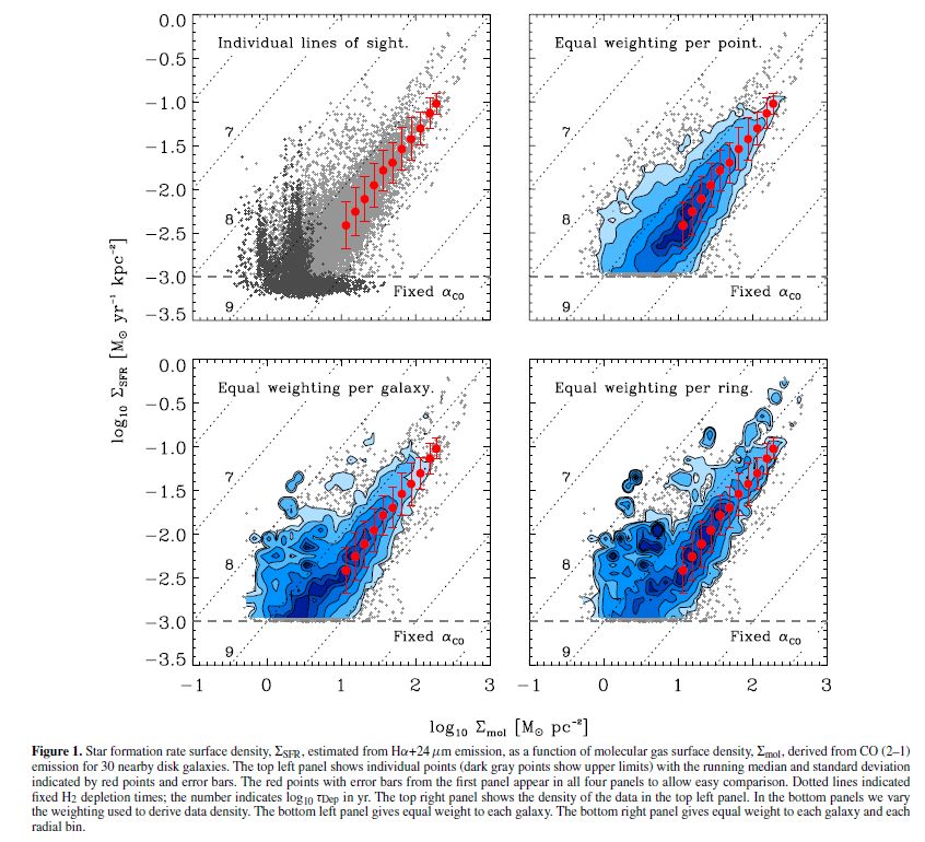
 normalizing per (projected) galaxy surface (requires that galaxies are
 (marginally resolved)
  gas mass per unit area
 Σ 
  star formation rate per
 unit area Σ 

 local galaxies:

 1.4
 Σ ∝ Σ 

 (slope may vary depending on
 SFR assumptions, XCO scaling,
 etc.)

Abbildung 1 Correlation between gas surface density and star
formation surface density , integrating over whole galaxies. Galaxy
classes are indicated in the legend (Kennicutt & Evans 2012)

 use of rotation curve:
 Σ / 
 has units of −1 −2

 similar to [Σ ] = −1 −2

 relation describes what fraction of
 gas is converted into stars per
 orbital period

Abbildung 2 Kennicutt (1998)

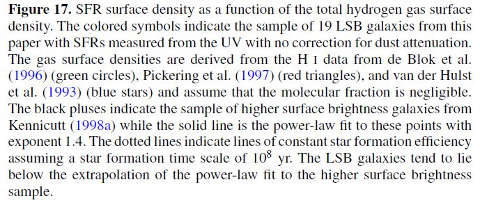
7.1.1.3 High Redshift Galaxies

 adding high z data suggests no
 single relationship but
  normal galaxies
  starburst galaxies

Abbildung 3 Daddi et al. 2010

 but normalizing to dynamical time
 scale still yields a strong
 correlation.

Abbildung 4 Daddi et al. 2010

7.1.1.4 Dwarfs and low surface brightness galaxies

 Only after GALEX (FUV) and Herschel
 (FIR) data was available this could
 be measured because dwarfs are
 too faint in H and the XCO factor is
 definitely different.
Abbildung 5 Wyder et al. 2009

Dwarfs fall below the Kennicutt- Schmidt law!

7.1.2 The Spatially-Resolved Star Formation Rate
Thanks to technological advances!
7.1.2.1 Relationship to Molecular Gas

@ 0.5-1 kpc => very good correlation between molecular gas and SFR

in inner disks of nearby galaxies (CO detectable) we find a roughly
constant depletion time
 ΣH 2
 = ≈ 2 Gyr
 ΣSFR

basically, insensitive to any other property of the galaxy, e.g. orbital time
scale!
Surprising since normalizing to tdyn reduced scatter Kennicutt-Schmidt
law.

Abbildung 6 Leroy et al. 2013

 (Krumholz 2014)

 normalizing K-S law by 

 (difficult to determine!)

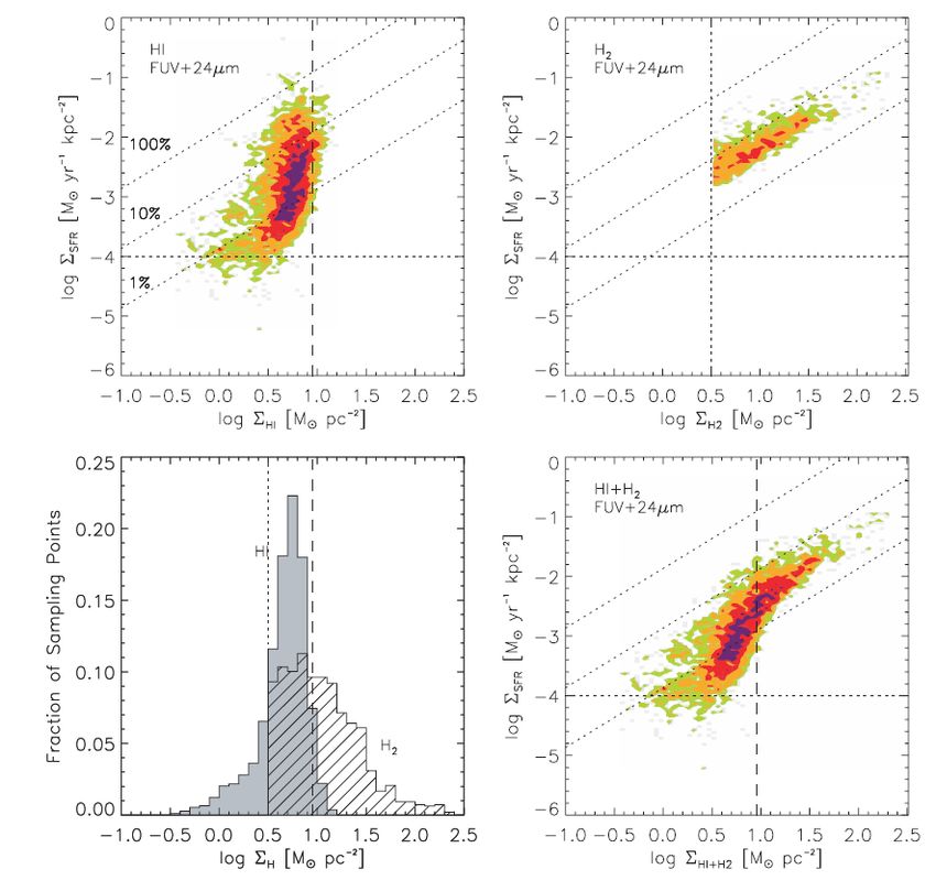
Caveats:
  limited to inner parts of galaxies with significant CO
  limited galaxy sample ≲ 20 Mpc (no starbursts in this volume)
  correlation strength depends on scales over which we average
 o on sufficiently small scales we do not look at an average piece
 of galaxy any more
 o proxies carry different information
 ▪ CO: momentaneous mol. gas content
 ▪ H : average # of stars formed in the last ~5Myr
 ▪ relating each other is misleading
 o on larger scales this averages out
 7.1.2.2 Relationship to Atomic Gas
 Very different results for total (or atomic) gas.
 HI surface density
 reaches a maximum is
 uncorrelated to SFR @
 this max.
 In inner parts of
 galaxies, SF does not
 care about atomic gas.

Abbildung 7 K-S law for HI gas in inner galaxies, averaged for ~ 750 pc scales (Bigiel et al.
2009)

 In contrast to that: in the outer parts of galaxies there seems to be a
 correlation to the HI gas

here very long
 ~100 Gyr

 probably result of very low
 H2-HI ratio of 1-2%

 because if CO is detectable
Abbildung 8 Bigiel et al. 2010, K-S-law for HI gas in outer galaxies on ~750 pc we still find
scales.
 , ~ 2 Gyr
When plotting SFR against mol. + atomic gas we find a clear correlation

 @ high Σ
 most gas is in H2
 ~2 Gyr

 @ low Σ
 most gas is in HI
 ~100 Gyr
 SFR drops by factor
Abbildung 9 Krumholz 2014
 of 50

7.1.3 Star Formation in dense gas
7.1.3.1 Alternatives to CO

So far: CO as H2 proxy
Next brightest mol. line in galaxies: HCN (HCO+, CS, and HNC)

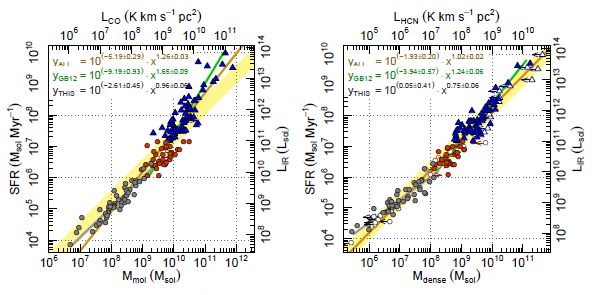
~10 times fainter than CO (100 x mapping times!)
Comparison:
 • Energy levels
 o CO: 5.5, 16.6, 33.3, 55.4 K
 o HCN: 4.3, 12.8, 25.6, 42.7 K
 • Coll. de-excitation rates for 1-0
 o CO: 10 = 3.3 × 10−11 cm3 s−1
 o HCN: 10 = 2.4 × 10−11 cm3 s−1
 • Einstein A-values for 1-0
 o CO: 10 = 7.2 × 10−8 s−1
 o HCN: 10 = 2.4 × 10−5 s−1
 • critical density for 1-0
 o CO: = 2200 cm−3
 o HCN: = 106 cm−3
HCN => tracer of dense gas!
Correlation with SFR but somewhat lower slope than with CO!

Abbildung 10 Usero et al. 2015

7.2 THEORY
Any successful theory needs to reproduce the main observational results:
 • SF appears to be very slow or inefficient ≈ 100 × 
 • in unresolved observations, the SFR rises non-linearly with total gas
 content
 • in central disks of galaxies SF correlates strongly with molecular gas
 and poorly with atomic gas
 • constant in nearby normal galaxies, shorter in actively
 star-forming galaxies
 • A correlation between SF and atomic gas only where the gas
 content is dominated by atomic phase. Then
 , . ≈ 100 × , 
 • If dense gas tracers are used is shorter than for the bulk of the
 molecular gas, but still much longer than 
At present, no theory explains all the observations!
 • top-down model: SF regulated by galactic-scale processes
 • bottom-up model: SF regulated within molecular clouds

7.2.1 The Top-Down approach
7.2.1.1 Hydrodynamics plus Gravity
Simplest ansatz: only hydrodynamics & gravity, no feedback
  baseline models
  study of large-scale gravitational instability
 Ω 
 = Toomre (1964) Q parameter
 Σ
Ω: angular velocity of disk rotation, : gas velocity dispersion, Σ: gas
surface density
 • 1 system stable
Observed galactic disks ≈ 1 for majority of disk and > 1 at edges

If ≈ 1: grav. instability (self-gravity of disk) occurring on galactic scale
might be an important driver of star formation.
If > 1: grav. instability unimportant on large scales, SF occurs locally,
where global structures (e.g. spiral waves) compress the gas.
 • Usually these models give ~1 (rather than 0.01) because nothing
 stops a collapse once it begins.
 • No dependence on metallicity (which is observed)
7.2.1.2 Feedback Regulated Models
Gas-momentum equation without viscosity and with magnetic fields:
 1 2
 ( ⃗) = −∇ ⋅ ( ⃗ ⃗) − ∇ + ⃗⃗ ⃗⃗
 ∇ ⋅ ( − ⃗) + ⃗
 4 2
disk in x-y plane. Only take z-component:
 d 1 1 2
 ( ) = −∇ ⋅ ( ⃗ ) − + ⃗⃗ ) −
 ∇ ⋅ ( + 
 4 8 
Consider some area at constant height , average over :
 1 d⟨ ⟩ 1
 ⟨ ⟩ = − ∫ ∇ ⋅ ( ⃗ ) − + ⃗⃗ ) 
 ∫ ∇ ⋅ ( 
 4 A
 1 2
 − ⟨ ⟩ + ⟨ ⟩ 1
 8 ⟨ ⟩ = ∫ 
 
separate xy components from z component in divergences (and apply
divergence theorem)
 d ⟨ ⟩ 1 2 1 2
 ⟨ ⟩ = − − ⟨ ⟩ + ⟨ ⟩ − ⟨ 2 ⟩ + ⟨ ⟩
 8 4 
 1 1
 − ∫ ∇xy ⋅ ( ⃗ ) + ⃗⃗ ) 
 ∫ ∇ ⋅ ( 
 4 A xy
 d ⟨ ⟩ 1 2 1 2
 ⟨ ⟩ = − − ⟨ ⟩ + ⟨ ⟩ − ⟨ 2 ⟩ + ⟨ ⟩
 8 4 
 1 1
 − ∫ ⃗ ̂ ℓ + ∫ ⃗⃗ ⋅ ̂ ℓ
 
 : boundary of , ̂: unit vector normal to boundary (always lies in xy
plane)

1
 ∫ ⃗ ̂ ℓ:
 
 advection of momentum across edges of the area

 if galaxy with no net flow in galaxy → 0
1
 ∫ ⃗⃗ ⋅ ̂ ℓ: rate at which z momentum is transmitted across
 
 boundary by magnetic stresses, again → 0
 
galactic disk ~ time steady: →0
 
Equation of hydrostatic balance for galactic disk:
 1 2 1 2
 ⟨ + 2 + ⟩− ⟨ ⟩ − ⟨ ⟩ = 0
 8 4 

 1
 ⟨ + 2 + 2 ⟩: upward force due to gradients in the total
 8 
 pressure, incl. turb. pressure 2 and magn.
 pressure 2 /4 
⟨ ⟩: downward force due to gravity
1 
 ⟨ 2 ⟩: forces due to magnetic tension (usually not
4 
 dominant).
⇒ balancing first and last term!
 
force ≡ ≡ momentum flux
 
Each term: rate (per unit area) at which momentum is transported up or
down.

Feedback Ansatz: rate in the first term = rate of momentum injected
 by feedback

 1 2 
 ⟨ + 2 + ⟩ ∼ ⟨ ⟩ Σ 
 8 

 
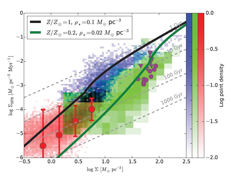
⟨ ⟩: momentum yield per unit mass of stars formed (includes any
 
feedback process we can come up with)

Gravity of an infinite slab of gas: = 2 Σ

 −1
 (⟨ ⟩ Σ ) ∼ 2 Σ ⇒ Σ ∼ 2 ( ) Σ Σ 
 
assuming ∼ 1/ℎ, therefore ℎ ∼ Σ 
 
In such a model we expect the SFR to scale with Σ Σ .
If the gas dominates the gravity:
 2
 Σ ∝ Σ 
If the stars dominate the gravity:
 Σ ∝ Σ Σ∗

If we know ( ) we can compute SFR quantitatively.
 
Example:
 
total momentum yield of supernovae: ( ) ∼ 3000 km s −1
 
 2
 Σ
 • Σ ∼ 0.09 M⊙ pc −2
 Myr −1
 ( )
 100 M⊙ pc−2

~ right magnitude for observed SFRs

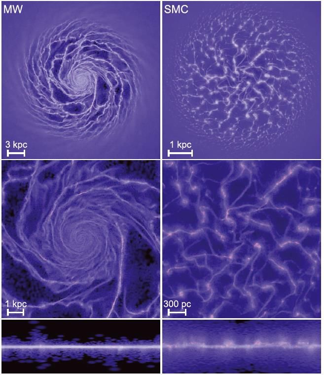
Abbildung 11 Hopkins et al. 2011: SFR versus time from simulations of isolated galaxies performed with (blue) and without (red) a
subgrid mode for stellar feedback. MW (Milky Way) SMC: Small Magellanic Clouds

 Successes:
 • physically motivated
 • allow quant.
 computation of SFR (in models
 and analytically)
 • SFR independent of
 microphysics and cloud scale
 processes
 • Σ ∝ Σ Σ∗ agrees
 with what we find in the outer
 MW.

Problems:
 
 • SFR predictions depends on assumptions about ( )
 
 • In the gas dominated case we expect Σ ∝ Σ 
 2
 , but we observe
 1.4
 (Kennicutt-Schmidt relation) ∝ Σ 
 • Even though the SFR in the outer MW matches the model
 predictions, the model doesn’t care about metallicity. But we
 observe a metallicity dependence
 • The feedback approach doesn’t distinguish between H and H2

• Observations suggest that SF is equally slow in clouds and in whole
 galaxies. In the feedback models this is not required. We can have
 fast SF in clouds and slow in the whole galaxy. But, then why do we
 observe a slow SFR where we have no feedback (as in the solar
 neighborhood)?

7.2.2 The Bottom-Up Approach
Start SF from individual clouds.
 • Which parts of a galaxy’s ISM are eligible to form stars
 • SFR within individual clouds
7.2.2.1 Which gas is star forming?
Observationally: stars form in molecular gas. -> Where is the mol. gas in a
galaxy?
Physical explanation?
H2 and CO are cooling more efficiently?
NO! C+ is as good as CO in cooling and not all H2 is associated with CO!

Instead: H2 is associated with SFR because of shielding!

Thermal balance in the ISM:
Main heating: photo-electric heating and cosmic-ray heating.
Total heating rate per H nucleus:
 Γ = (4 × 10−26 ′ − + 2 × 10−27 ′ ) erg s−1
 : local FUV radiation field
 ′ : local dust metallicity
 ′ : CR ionization rate
 : dust optical depth
If CO has not yet formed -> C+ main coolant ([CII] 158µm fine structure
line, 92 K)

opt. thin gas, LTE: cooling rate Λ
 Λ CII = CII−H C CII 
 CII−H ≈ 8 × 10−10 − CII/ : excitation (by collisions) rate coefficient
 CII = 91 : energy of excited state
 C ≈ 1.1 × 10−4 ′ : carbon abundance relative to hydrogen
 CII = CII : energy of the level
 H : hydrogen number density

From Γ = Λ we find :
 CII
 =−
 − 0.018 ′
 ln (0.36 FUV + ) − ln H,2
 ′
 H
 H,2 =
 100 cm−3

If FUV heating dominates:
 91K
 ≈
 1.0 + − ln FUV + ln H,2
If CR heating dominates:
 91K
 ≈
 4.0 − ln ′ / ′ + ln H,2
Transition at ∼ 3
 ′
CR dominated regime ( = 1) => T=23K (almost as low as in the CO
 ′
dominated region with T~10K)
FUV dominated regime and low opt. depth => T~100 K
Jeans mass:
 3/2
 3
 2 −1/2 3/2
 = = ( ) = 4.8 × 103 ⊙ 2
 

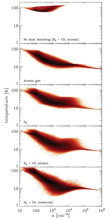
 93 1.5
( 2 = ), so will differ by ( ) ≈ 8.
 100 23

  high (suppresses FUV heating) and lowers the mass that is stable
 against collapse (by ~ one order of magnitude)

Bottom-up models: this change in as a function of regulates the SF
In warm regions (by FUV heating) the gas is thermally stabilized
In cold regions SF proceeds efficiently

 Left: n-T distribution in simulations
 with different treatments of the
 ISM (Glover and Clarke 2012)
 All simulations use identical initial
 conditions, but vary in how the gas
 heating and cooling rates are
 calculated. The top panel ignores
 dust shielding, but includes full
 chemistry and heating and cooling.
 The bottom panel includes all
chemistry and cooling. The middle three panels turn off, respectively, H2
formation, CO formation, and CO cooling. The tail of material proceeding
to high density in some simulations is indicative of star formation.

Relation to H2: H2 depends on FUV shielding
shielding column of hydrogen before H2 can be formed:
 0∗ −1 ( ′ )−1
 H = ≈ 7.5 × 1020 FUV H,2 cm−2
 ℛ
or
 −1 ( ′ )−1
 ΣH = H H = 8.4 FUV H,2 M⊙ pc −2
This corresponds to an optical depth at which the gas becomes molecular:
 −1
 = H = 7.5 FUV H,2 ( ′ )−1
( ≈ 10−21 ′ −2 ). About the same opt. depth at which the transition
from FUV to CR dominated heating occurs.
 −1
 FUV H,2 ~few × 10−1 : ~ const. in the MW disk because of ISM two-
phase equilibrium.
  physical explanation why SF is correlated to molecular gas
  physical reason for breakdown at ΣH ≤ 10 M⊙ pc −2
  metallicity dependence is also explained

7.2.2.2 The Star Formation Rate in Star-Forming Clouds
Overall SFR? Why is the SFR so low?
Turbulent support:

Consider a turbulent medium with linewidth-size relation
 1/2
 ( ) = ( )
 
 : sonic length. What parts of this flow will become Jeans-unstable.
The max. mass that can be held up against turbulence: Bonnor-Ebert
mass:
 3 1.18
 = 1.18 3 = 3 3
 
 2
 : isothermal sound speed, : local gas density (density at the surface of
the Bonnor-Ebert sphere). The corresponding radius is:
 = 0.37 
 a: geometric factor
Virial terms: (a=0.73 max. mass sphere)
 2
 5
gravitational energy: = − = −1.06
 3/2 1/2
 3
Thermal energy: ℎ = 2 = 1.14 | |
 2
 3 
Turbulent energy: = (2 )2 = 0.89 ( ) | |
 2 

  Collapsing parts of the flow where the density is very high
  ≳ 
  ≲ 

  Ansatz: Collapse if: ≲ 

 2 Jeans length at the mean density
 0 =√
 ̅

 = / ̅ , then = 0 /√ 

 0 2 ~1
 ≲ then requires > ≡ ( )
 
mass fraction where ≲ 

 2
 ∞
 1 ∞ ̅̅̅̅̅
 (ln − ln )
 =∫ = ∫ exp [− 2 ] 
 ln 2 2 
 √2 
 1 −2 ln + 2 3ℳ 2
 1/2
 = [1 + erf ( )] ≈ [ln (1 + )]
 2 23/2 4

assume a fraction collapses every free-fall time, then the SFR per is

 1 −2 ln + 2 ~1
 = [1 + erf ( )]
 2 23/2 

more detailed (Hennebelle & Chabrier, Federrath & Klessen):
 1 ∞ 1/2
 = ∫ 
 ln 
 1 − ln + 2 3 2
 = [1 + erf ( )] exp ( )
 2 21/2 8 

 0
 : from observations:
 
 5 2 
In regions where =
 
 1/2 2
then ( ) = 2 ( ) and therefore = 2 ( )
 2 2 

 2 3
and 0 = √ = 2 √
 3 

 0 2 2 
 2
together: = ( ) = ℳ 2 ≈ 0.82 ℳ 2
 15

For ≈ 2, ≈ 0.1 (observed ≈ 0.01) Assuming some local
feedback that decreases further puts it in the right order.

7.2.2.3 Strengths and Weaknesses of the Bottom-Up Models
  B-U models reproduce SFR-ISM phase dependence
  B-U models explain metallicity dependence
  B-U reproduces ≈ 0.01 on all scales

  why ≈ 0.01 instead of ≈ 0.1 is not fully explained
  global regulation of the ISM and its hydro-balance not addressed
 (where does the initial hydrostatic balance comes from?)