Theory of Proton-Coupled Electron Transfer
←
→
Page content transcription
If your browser does not render page correctly, please read the page content below

Theory of
Proton-Coupled Electron Transfer
                        Sharon Hammes-Schiffer
                      Pennsylvania State University
                                  ET
                                           PT
                 De          Dp        H        Ap       Ae

                                       R

Note: Much of this information, along with more details, additional rate
constant expressions, and full references to the original papers, is available
in the following JPC Feature Article:
Hammes-Schiffer and Soudackov, JPC B 112, 14108 (2008)

Copyright 2009, Sharon Hammes-Schiffer, Pennsylvania State University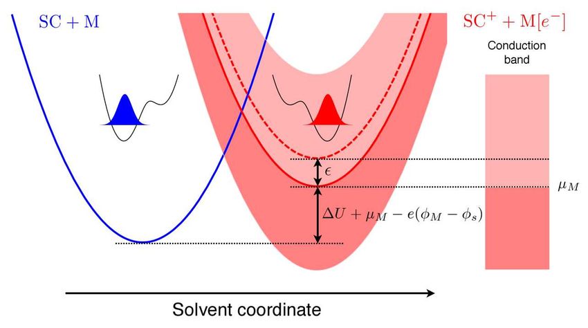
General Definition of PCET
                         ET
                                  PT
           De       Dp        H        Ap   Ae

                              R
• Electron and proton transfer reactions are coupled
• Electron and proton donors/acceptors can be the same or
  different
• Electron and proton can transfer in the same direction
  or in different directions
• Concerted vs. sequential PCET discussed below
• Concerted PCET is also denoted CPET and EPT
• Hydrogen atom transfer (HAT) is a subset of PCET
• Distinction between PCET and HAT discussed below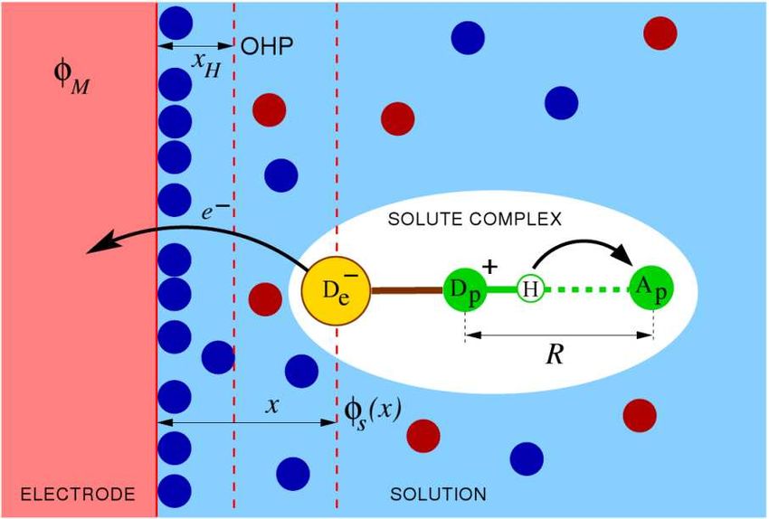
Examples of Concerted PCET

     ET

     PT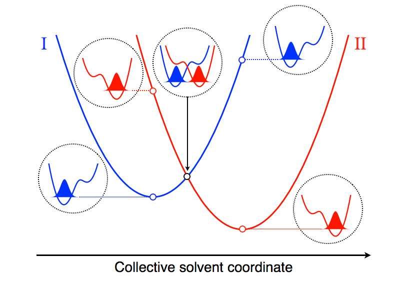
Importance of PCET

• Biological processes
    − photosynthesis          Cytochrome c oxidase
    − respiration             4e− + 4H+ + O2 → 2(H2O)
    − enzyme reactions
    − DNA

• Electrochemical processes
    − fuel cells
    − solar cells
    − energy devices
Theoretical Challenges of PCET
• Wide range of timescales
   − Solute electrons
   − Transferring proton(s)
   − Solute modes
   − Solvent electronic/nuclear polarization
• Quantum behavior of electrons and protons
   − Hydrogen tunneling
   − Excited electronic/vibrational states
   − Adiabatic and nonadiabatic behavior
• Complex coupling among electrons, protons, solvent
Single Electron Transfer
Diabatic states: Marcus theory
(1) D e− A e
(2) D e A e−
Solvent coordinate
ze = ∫ dr ( ρ 2 − ρ1 )Φ in (r )
Nonadiabatic ET rate: k = 2π V122 (4πλ kBT )−1/ 2 exp − ∆G † (k BT )
ℏ
∆G † = ( ∆G + λ ) ( 4λ )
2
V12 : coupling between diabatic states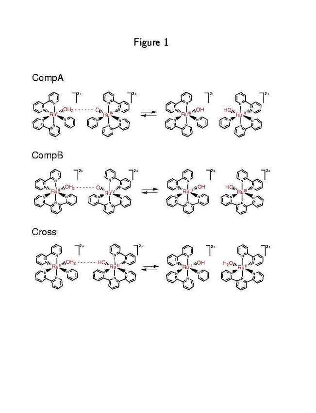
Inner-Sphere Solute Modes
2π 2 2
k= V12 (4πλ k BT ) −1/ 2 ∑ PµI ∑ ϕ µ(1) | ϕυ(2) exp − ∆G1†µ ,2υ (k BT )
ℏ µ υ
vibrational wavefunctions ϕ µ(1) , ϕυ(2)
Assumes solute mode is not coupled to solvent →
Not directly applicable to PCET because proton strongly
coupled to solvent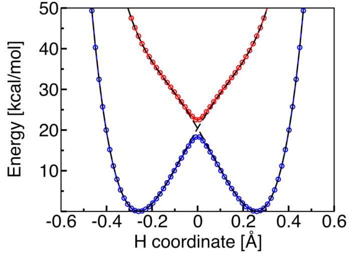
Single Proton Transfer
   Diabatic states:            Solvent coordinate
    (a ) D p H + A p−            z p = ∫ dr ( ρb − ρ a )Φ in (r )
    (b ) D p   HA p            Proton coordinate: rp (QM)

PT typically electronically adiabatic (occurs on ground electronic
state) but can be vibrationally adiabatic or nonadiabatic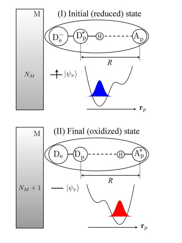
Proton-Coupled Electron Transfer
Soudackov and Hammes-Schiffer, JCP 111, 4672 (1999)
− +
• Four diabatic states: (1a ) D e D p H ⋯⋯ A p A e
(1b ) D e− D p ⋯⋯ HA +p A e
(2 a ) D e + D p H ⋯⋯ A p A e−
(2b ) D e D p ⋯⋯ HA p+ A e−
• Free energy surfaces depend on 2 collective
solvent coordinates zp, ze
PT (1a ) → (1b): z p = ∫ dr ( ρ1b − ρ1a )Φ in (r )
ET (1a ) → (2a ) : ze = ∫ dr ( ρ 2 a − ρ1a )Φ in (r )
• Extend to N charge transfer reactions with 2N states and N
collective solvent coordinates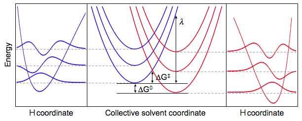
Sequential vs. Concerted PCET (1a ) D e− + D p H ⋯⋯ A p A e (1b ) D e− D p ⋯⋯ HA p+ A e (2 a ) D e + D p H ⋯⋯ A p A e− (2b ) D e D p ⋯⋯ HA +p A e− • Sequential: involves stable intermediate from PT or ET PTET: 1a → 1b → 2b ETPT: 1a → 2a → 2b • Concerted: does not involve a stable intermediate EPT: 1a → 2b • Mechanism is determined by relative energies of diabatic states and couplings between them • 1b and 2a much higher in energy → concerted EPT
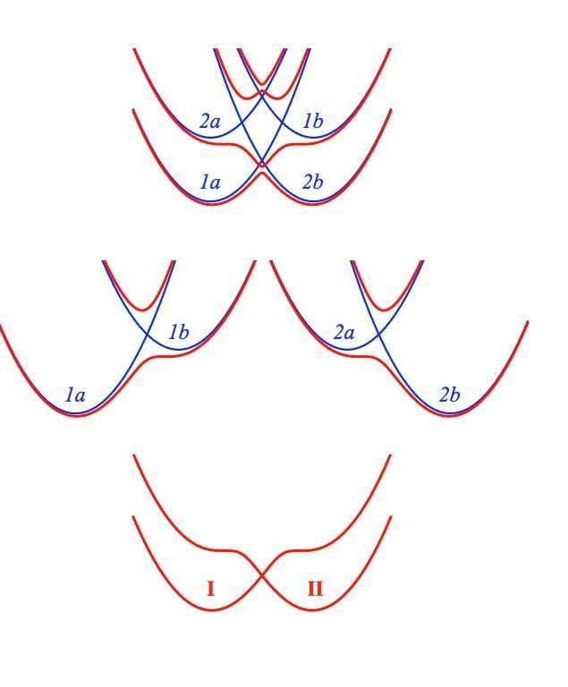
Reactant and Product Diabatic States
Remaining slides focus on “concerted” PCET:
describe in terms of Reactant → Product

• Reactant diabatic state (I)
  - electron localized on donor De
  - mixture of 1a and 1b states

• Product diabatic state (II)
  - electron localized on acceptor Ae
  - mixture of 2a and 2b states

Typically large coupling between a and b PT states and
smaller coupling between 1 and 2 ET states
Diabatic vs. Adiabatic Electronic States
               4 diabatic states: 1a, 1b, 2a, 2b
               4 adiabatic states:
               Diagonalize 4×4 Hamiltonian matrix in basis
               of 4 diabatic states
               Typically highest 2 states can be neglected

                      2 pairs of diabatic states: 1a/1b, 2a/2b
                      2 pairs of adiabatic states:
                      Block diagonalize 1a/1b, 2a/2b blocks
                      Typically excited states much higher
                      in energy and can be neglected

               2 ground adiabatic states from block
               diagonalization above:
               Reactant (I) and Product (II) diabatic states
               for overall PCET reaction
Electron-Proton Vibronic States H treated quantum mechanically Calculate proton vibrational states for electronic states I and II - electronic states: ΨI(re,rp), ΨII(re,rp) - proton vibrational states: ϕIµ(rp), ϕIIν(rp) Reactant vibronic states: ΦI(re,rp) = ΨI(re,rp) ϕIµ(rp) Product vibronic states: ΦII(re,rp) = ΨII(re,rp) ϕIIν(rp) Coupling between reactant and product vibronic states typically much smaller than thermal energy because of small overlap → Describe reactions in terms of nonadiabatic transitions between reactant and product vibronic states Vibronic states depend parametrically on other nuclear coords
2D Vibronic Free Energy Surfaces

                             Reactant (1a/1b)   D−    A

                             Product (2a/2b)    D     A−

• Multistate continuum theory: free energy surfaces depend
  on 2 collective solvent coordinates, zp (PT) and ze (ET)
• Mixed electronic-proton vibrational (vibronic) surfaces
• Two sets of stacked paraboloids corresponding to different
  proton vibrational states for each electronic state
One-Dimensional Slices
• Shape of proton potentials not
significantly impacted by solvent
coordinate in this range
• Relative energies of reactant and
product proton potentials strongly
impacted by solvent coordinate
Mechanism:
1.System starts in thermal equilibrium on reactant surface
2.Reorganization of solvent environment leads to crossing
3.Nonadiabatic transition to product surface occurs with
probability proportional to square of vibronic coupling
4. Relaxation to thermal equilibrium on product surfaceFundamental Mechanism for PCET Solvent Coordinate rp
Fundamental Mechanism for PCET

  Solvent Coordinate   rp
Fundamental Mechanism for PCET

  Solvent Coordinate   rp
Overview of Theory for PCET
Hammes-Schiffer, Acc. Chem. Res. 34, 273 (2001)
ET
PT
De Dp H Ap Ae
R
• Solute: 4-state model (1a ) De− + D p H ⋯⋯ A p A e
(1b) De− D p ⋯⋯ HA p+ A e
(2a ) De + D p H ⋯⋯ A p A e−
(2b) De D p ⋯⋯ HA +p A e−
• H nucleus: quantum mechanical wavefunction
• Solvent/protein: dielectric continuum or explicit molecules
• Typically nonadiabatic due to small coupling
• Nonadiabatic rate expressions derived from Golden RulePCET Rate Expression
Soudackov and Hammes-Schiffer, JCP 113, 2385 (2000)
Reactant (1a/1b) D− A
Product (2a/2b) D A−
2π
∑ PµI ∑ ( 4πλµν kBT )
−1/2 2
k= Vµν exp − ∆Gµν
†
(k BT )
ℏ µ ν
∆Gµν = ( ∆Gµν + λµν ) ( 4λ )
† 2
µν
Vµν = Φ I ( re , rp ) Hˆ Φ II (r , r )
e p ≈ V el S µν
H coordinateExcited Vibronic States
2π
∑ Pµ ∑ ( 4πλµν kBT )
−1/ 2 2
k= I
Vµν exp − ∆Gµν
†
(k BT )
ℏ µ ν
Relative contributions from excited vibronic states determined
from balance of factors (different for H and D, depends on T)
• Boltzmann probability of reactant state
• Free energy barrier
• Vibronic couplings (overlaps)
V ETProton Donor-Acceptor Motion
R
De Dp H Ap Ae
• R is distance between proton donor and acceptor atoms
• R-mode corresponds to the change in the distance R,
typically at a hydrogen-bonding interface
• R-mode can be strongly influenced by other solute nuclei,
viewed as the “effective” proton donor-acceptor mode
ET
V
• PCET rate is much more sensitive to R than to electron
donor-acceptor distance because of mass and length
scales for PT compared to ET
For this PCET reaction, R is distance
between donor O and acceptor N in
PT reactionRole of H Wavefunction Overlap
R
De Dp H Ap Ae
• Rate decreases as overlap decreases (as R increases)
k H ∝ VH2 ∝ ( H overlap) 2
• KIE increases as overlap decreases (as R increases)
k H VH2 ( H overlap) 2
∝ 2 ≈ (for a pair of vibronic states)
k D VD ( D overlap) 2
solid: H
dashed: DInclude Proton Donor-Acceptor Motion
Soudackov, Hatcher, SHS, JCP 122, 014505 (2005)
R
De Dp H Ap Ae
• Vibronic coupling (overlap) depends strongly on R
• Approximate vibronic coupling as
Vµν ( R ) ≈ V el S µν
0
exp −α µν ( R − Req )
ET
Vel: electronic coupling V
0
S µν : proton wavefunction overlap at Req
Req: equilibrium R value
• Derived dynamical rate constant with quantum R-mode and
explicit solvent
• Derived approximate forms for low- and high-frequency R-mode
using a series of well-defined approximationsDynamical Rate for Molecular Environment
∞
1
kdyn = 2
ℏ ∫ j ( t ) dt
−∞
i
j ( t ) = V S µν exp E t
el 0 2
ℏ
2iα
t
× exp α 2 CR ( 0 ) + CR ( t ) − Dɶ ∫ C (τ ) dτ
R
ℏ 0
τ1 τ1
1
t
1
t
− 2 ∫ dτ 1 ∫ dτ 2CE (τ 1 − τ 2 ) − 2 ∫ dτ 1 ∫ dτ 2CD (τ 1 − τ 2 ) CR (τ 1 − τ 2 )
ℏ 0 0
ℏ 0 0
V ETɶ ∂∆ε
Energy gap and its derivative: E ( t ) = ∆ε ( Req , ξ ( t ) ) D =
∂R R = Req
Time correlation functions: CR ( t ) , CE ( t ) , CD ( t )
• Calculate quantities with classical MD on reactant surface
• Includes explicit solvent/protein environment
• Includes dynamical effects of R-mode and solvent/protein
Soudackov, Hatcher, SHS, JCP 2005Closed Analytical Rate Constant
Approximations: short-time, high-T limit for solvent and
quantum harmonic oscillator R-mode
2
∞
V el S µν 2λ ζ
0
k = ∑ Pµ ∑
I
exp α ∫ dτ exp − χτ 2 2 + p(cos τ − 1) + i (q sin τ + θτ
µ ν ℏ2Ω ℏΩ −∞
Parameters depend on T, reorganization energies, reaction
free energies, vibronic coupling exponential Vfactor,
ET mass and
frequency of R-mode, and difference in product and reactant
equilibrium R values
Rate constant expressed in terms of physically meaningful
parameters but requires numerical integration over time
Soudackov, Hatcher, SHS, JCP 2005High-Frequency R-mode
Ω >> kBT
( ∆Gµν + λ )
2 2
π λα − λR
el 0 0
V S µν
k = ∑ Pµ ∑ I
exp − α µν δ R exp −
µ ν ℏ λ kBT ℏΩ 4λ kBT
ℏ 2α µν
2
M, Ω: mass and frequency of R-mode
λα = α: exponential R-dependence of vibronic coupling
2M
δ R = M Ω2δ R 2 2 δR: difference between product and reactant
equilibrium values of R
Assumption of derivation (strong-solvation limit): λ > ∆Gµν
0
In this limit, sole effect of R-mode on rate constant is that
vibronic coupling is averaged over ground-state vibrational
wavefunction of R-mode
For very high Ω, use fixed-R rate constant expressionLow-Frequency R-mode Ω
Reorganization Energies
• Reorganization energy λ in previous expressions refers to
   solvent/protein reorganization energy (outer-sphere)
• Inner-sphere reorganization energy (intramolecular solute
  modes) can also be included
  - high-T limit (low-frequency modes): add inner-sphere
    reorganization energy to solvent reorganization energy
  - low-T limit (high-frequency modes): modified rate constant
    expression has been derived
  (Soudackov and Hammes-Schiffer, JCP 2000)
• Calculation of reorganization energies
  - Outer-sphere: dielectric continuum models or molecular
     dynamics simulations
  - Inner-sphere: quantum mechanical calculations on solute
Input Quantities • Reorganization energies (λ) - outer-sphere (solvent): dielectric continuum model or MD - inner-sphere (solute modes): QM calculations of solute • Free energy of reaction for ground states (driving force) (∆G0) - QM calculations or estimate from pKa’s and redox potentials • R-mode mass and frequency (M, Ω) - QM calculation of normal modes or MD - R-mode is dominant mode that changes proton donor-acceptor distance • Proton vibrational wavefunction overlaps (Sµν , αµν) - approximate proton potentials with harmonic/Morse potentials or generate with QM methods - numerically calculate H vibrational wavefunctions w/ Fourier grid methods • Electronic coupling (Vel) - QM calculations of electronic matrix element or splitting Note: this is a multiplicative factor that cancels for KIE calculations
Warnings about Prediction of Trends
           Edwards, Soudackov, SHS, JPC A113, 2117 (2009)

• Experimentally challenging to change only a single parameter
  Examples:
 Increasing R often decreases Ω; may impact KIE in opposite way
 Changing driving force by altering pKa can also impact R
• Relative contributions from pairs of vibronic states are
  sensitive to parameters, H vs. D, and temperature
 Must perform full calculation (converging number of reactant and product
 vibronic states) to predict trend
• High-frequency and low-frequency R-mode rate constants
  are qualitatively different
 Example:
 Low-frequency expression predicts KIE decreases with T
 Fixed-R and high-frequency expressions can lead to either increase
 or decrease of KIE with T
Driving Force Dependence
Edwards, Soudackov, SHS, JPC A 2009; JPC B 113, 14545 (2009)
Free energy vs. Solvent coordinate
−∆G 0 < λ −∆G 0 > λ
• Theory predicts inverted region behavior V ET
not experimentally accessible for PCET
due to excited vibronic states with
enhanced couplings
• Apparent inverted region behavior could be
observed experimentally if changing driving force also impacts
other parameters (e.g., increasing |∆pKa| also increases R)Applications to PCET Reactions
• Amidinium-carboxylate salt bridges (Nocera), JACS 1999
• Iron bi-imidazoline complexes (Mayer/Roth), JACS 2001
• Ruthenium polypyridyl complexes (Meyer/Thorp), JACS 2002
• DNA-acrylamide complexes (Sevilla), JPCB 2002
• Ruthenium-tyrosine complex (Hammarström), JACS 2003
• Soybean lipoxygenase enzyme (Klinman), JACS 2004, 2007
• Rhenium-tyrosine complex (Nocera), JACS 2007
• Quinol oxidation (Kramer), JACS 2009
• Osmium aquo complex/SAM/gold electrode (Finklea), JACS 2010
Experimental groups in parentheses, followed by journal and year of
Hammes-Schiffer group application
Theory explained experimental trends in rates, KIEs, T-dependence,
pH-dependence
ET
PTDistinguishing between HAT and PCET
Skone, Soudackov, SHS, JACS 128, 16655 (2006)
• Overall HAT and PCET usually vibronically nonadiabatic since
vibronic coupling much less than thermal energy: Vµν τp
• HAT ↔ electronically adiabatic PT
PCET ↔ electronically nonadiabatic PTQuantify Nonadiabaticity: Vibronic Coupling
Georgievskii and Stuchebrukhov, JCP 2000; Skone, Soudackov, SHS, JACS 2006
( sc )
VDA = κVDA
(ad)
Electronically nonadiabatic PT:κ ≈ 2π p , p > 1
m
( ad )
VDA = ∆/2
Vc : energy at crossing point
E : tunneling energy (vibrational ground state)
τeRepresentative Chemical Examples
Phenoxyl/Phenol and Benzyl/Toluene self-exchange reactions
DFT calculations and orbital analysis:
Mayer, Hrovat, Thomas, Borden, JACS 2002
benzyl/toluene phenoxyl/phenol
C---H---C O---H---O
SOMO
DOMO
HAT PCET
ET and PT between ET and PT between
same orbitals different orbitalsPCET vs. HAT: Adiabaticity Parameter
Skone, Soudackov, SHS, JACS 2006
Benzyl-toluene: C---H---C, electronically adiabatic PT, HAT
p ≈ 4, τ p ≈ 4τ e
V el = 14, 000 cm -1
(sc)
VDA ≈ VDA
(ad)
=∆ 2
Phenoxyl-phenol: O---H---O, electronically nonadiabatic PT, PCET
p ≈ 0.01, τ e ≈ 80τ p
V el = 700 cm −1
(sc)
VDA ≈ VDA
(na)
= V el ϕ D(1) | ϕ A(2)Electrochemical PCET Theory
Venkataraman, Soudackov, SHS, JPC C 112, 12386 (2008)
Derived expressions for current densities j(η)
• Current densities obtained by explicit integration over x
∞
ja = F ∫ dx CSC ( x ) ka ( x )
xH
• Gouy-Chapman-Stern model for double layer effectsRate Constants for Electrochemical PCET
• Nonadiabatic transitions between electron-proton vibronic states
• Integrate transition probability over ε, weighting by Fermi
distribution and density of states for metal electrode
ka ( x ) = ∫ d ε 1 − f ( ε ) ρ ( ε ) Wa ( x, ε )
• Similar transition probabilities with modified reaction free energy:
∆Gµν ( x, ε ) ≈ ∆U µν − ∆U 00 + ε − eη + eφs ( x )Characteristics of Electrochemical PCET
• pH dependence: buffer titration, kinetic complexity, H-bonding
• Kinetic isotope effects Req
• Non-Arrhenius behavior at high T
De Dp Ap
• Asymmetries in Tafel plots, αΤ ≠ 0.5
H
at η=0 (observed experimentally)
δReq = 0
Effective activation energy contains δReq = 0.05 Å
T-dependent terms ±2α µν δ Req kBT
due to change in Req upon ET;
different sign for cathodic
and anodic processes →
asymmetries in Tafel plots
Cathodic transfer coefficient:
α T (η = 0) ≈ 0.5 − α 00δ Req kBT Λ 00
Venkataraman, Soudackov, SHS, JPC C 2008Photoinduced PCET
Venkataraman, Soudackov, SHS, JCP 131, 154502; JPC C 114, 487 (2009)
Homogeneous Interfacial: molecule-semiconductor interface
• Developed model Hamiltonian
• Derived equations of motion for reduced density matrix
elements in electron-proton vibronic basis
• Enables study of ultrafast dynamics in photoinduced processesBeyond the Golden Rule
Navrotskaya and Hammes-Schiffer, JCP 131, 024112 (2009)
• Derived rate constant expressions that interpolate between
golden rule and solvent-controlled limits
• Includes effects of solvent dynamics
• Golden rule limit
- weak vibronic coupling, fast solvent relaxation
- rate constant proportional to square of vibronic coupling,
independent of solvent relaxation time
• Solvent-controlled limit
- strong vibronic coupling, slow solvent relaxation
- rate constant independent of vibronic coupling,
increases as solvent relaxation time decreases
• Interconvert between limits by altering physical parameters
• KIE behaves differently in two limits, provides unique probewebPCET
http://webpcet.chem.psu.edu
• Interactive Java applets allow
users to perform calculations on
model PCET systems and
visualize results
• Harmonic, Morse, or general
proton potentials
• “Exact”, fixed R, low-frequency
or high-frequency R-mode rate
constant expressions
• Plot dependence of rates and
KIEs as function of temperature
and driving force
• Analyze contributions of vibronic
states
• Access via free registrationYou can also read