Stress-based topology optimization of compliant mechanisms using nonlinear mechanics
←
→
Page content transcription
If your browser does not render page correctly, please read the page content below
Mechanics & Industry 21, 304 (2020)
                                                                                                                            Mechanics
 c G. Capasso et al., Published by EDP Sciences 2020
https://doi.org/10.1051/meca/2020011
                                                                                                                           &Industry
                                                                                                                             Available online at:
                                                                                                                          www.mechanics-industry.org

    REGULAR ARTICLE

Stress-based topology optimization of compliant mechanisms
using nonlinear mechanics
Gabriele Capasso 1, * , Joseph Morlier 2 , Miguel Charlotte 2 , and Simone Coniglio 2,3
1
    DMSM, ISAE-SUPAERO, 10 Avenue Edouard Belin, Toulouse, France
2
    Univ Toulouse, ISAE Supaero-INSA-Mines Albi-UPS, CNRS UMR5312, Institut Clément Ader, Toulouse, France
3
    Airbus Operations SAS, 316 Route de Bayonn, 31300 Toulouse, France

              Received: 12 July 2019 / Accepted: 29 January 2020

              Abstract. The present work demonstrates how a light structure can be easily designed through Topology
              Optimization even including complex analysis and sizing criteria such as hyperelastic Neo-Hookean materials
              for nonlinear analysis and aggregated stress constraints. The SIMP approach was adopted and two different
              strategies were analysed using an in house versatile MATLAB code. MMA was used as reference optimizer (in
              structural optimization) whereas a unified aggregation and relaxation method was adopted to deal with stress
              constraints. Feasibility was analyzed from the viewpoint of allowable stress verification. Two test cases are then
              studied: a morphing airfoil (for aeronautical applications) and a geometric inverter (for mechanics and bio-
              medical applications). For both, a hyperelastic Neo-Hookean material was chosen. Finally a complementary
              study on the effects of constraints and the input force intensity is also presented.

              Keywords: Topology optimization / Nonlinear mechanics / Stress-based optimization / Morphing /
              Compliant mechanism

1 Introduction                                                                focuses on the SIMP approach and the code developed in
                                                                              our study is largely inspired by the top88.
The past twenty years have seen increasingly rapid                               In the literature, several promising applications of TO
advances in the field of structural optimization: in par-                     to classical aerospace structures can be found [9–13].
ticular, Topology Optimization (TO) is becoming a key                         Recently, researchers have shown an increased inter-
figure in the research panorama. This method leads to                         est in alternative architectures presenting wings with a
an optimal structural efficiency, through the removal of                      variable geometry, better known as “morphing wings”
unnecessarily placed material, in order to accomplish the                     [14–17]. Different types of morphing have been tested
minimization of a given objective (such as the compli-                        both numerically [18] and experimentally [19], reveal-
ance of the system). Since the pioneering work of Bendsoe                     ing the advantages in terms of aerodynamic drag, noise
and Kikuchi (1988) [1] a number of approaches have been                       and vibration control with respect to conventional air-
proposed, among which are: density-based methods (the                         craft configuration, based on flight control surfaces. Two
well-known SIMP algorithm) [2,3], evolutionary strategies                     main categories can be distinguished [20]: planform mor-
[4] and level-set based methods [5,6].                                        phing, based on the modification of the plant itself of the
   Moreover, several researchers have tried to implement                      wing, and performance morphing, which leads to variat-
and diffuse simple and efficient codes. One of the most                       ing the airfoil in shape (shape morphing) or in incidence
well-known and important results is due to Andreassen                         (twist morphing). In this paper, a shape morphing design
et al. [7], who created a very simple and efficient 88-line                   is analyzed.
code written in MATLAB, capable of optimizing an MBB                             Earlier work on TO was restricted to linear struc-
beam through a SIMP algorithm. Compared to other                              tural designs. Recent research explored the influence of
available codes and the same 99-line code (published by                       nonlinear mechanics on the TO in several simple applica-
Sigmund et al. [8]), the former needs much less computa-                      tions, including geometrical nonlinearity [21–24], material
tional power, thanks to judicious use of vectorization and                    nonlinearity [25–30] and both geometrical and material
pre-allocation of most of the variables. The present work                     nonlinearities simultaneously [31–33]. Work from [24] evi-
                                                                              dences the differences encountered in a TO problem,
                                                                              according to the choice of a linear or a nonlinear analysis,
     *   e-mail: gabriele.capasso@student.isae-supaero.fr                     leading to totally different results.

    This is an Open Access article distributed under the terms of the Creative Commons Attribution License (http://creativecommons.org/licenses/by/4.0),
                  which permits unrestricted use, distribution, and reproduction in any medium, provided the original work is properly cited.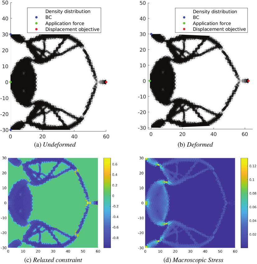
2                                      G. Capasso et al.: Mechanics & Industry 21, 304 (2020)

   The introduction of Nonlinear Mechanics into the               the different test-cases, outlining the relative mathemati-
TO of a morphing wing has already been treated by                 cal formalization. Optimized designs and numerical results
Bhattacharyya et al. [9]: in particular, geometric and            are finally reported and discussed in Section 5.
material nonlinearities have been investigated. In [9], the
optimization problem presents the objective of minimizing
the actuating force, under constraints of desired volume          2 Theoretical background
fraction, compliance and trailing edge displacement. The
obtained structure is, in fact, a compliant mechanism             In this section the basic principles of nonlinear mechanics
capable of getting a geometric advantage. The first of            and Topology Optimization are explored.
the two parts of the present work focuses on the same
structure, whilst the objective is to design the lightest         2.1 Nonlinear mechanics
structure under stress constraints, in order to conceive a
feasible structure.                                               The present work focuses on the design of large-
   In recent years other compliant mechanisms have fre-           displacement mechanisms, in which material doesn’t fol-
quently been proposed for aerospace systems due to their          low traditional linear mechanics. This topic will be just
advantages over traditional rigid-link mechanisms. As             introduced in this section, although it is largely explained
compliant mechanisms can be manufactured using fewer              in [43].
parts (usually one single part), they are lighter than their         Mechanical nonlinearities are distinguishable into four
traditional counterparts. They are also easy to manufac-          main categories [43]: (1) geometric nonlinearity (nonlinear
ture with modern 3D printing techniques, and do not               strain-displacement relation), (2) material nonlinearity
require assembly. The ability to 3D print mechanisms and          (nonlinear constitutive relation), (3) kinematic nonlin-
tools on board the International Space Station (or future         earity (non-constant displacement BCs, contact) and (4)
bases on the Moon and Mars) will save substantially on            force nonlinearity (follow-up loads).
the cost and time involved in transporting these devices             The resolution of a Nonlinear Finite Element Anal-
from Earth. To be prepared for deep-space exploration             ysis (NFEA) is not straight-forward, since the global
and habitation in the future, research and technology             system is nonlinear: in [43] several methods are illus-
development concerning the utilization of additively con-         trated. The most common algorithm is the one which
struct structures from insitu materials is incorporated into      goes under the name of Newton-Raphson, which is usually
the in-space manufacturing technology roadmap [34].               modified through the introduction of a step-force control.
   A compliant mechanism has been investigated by                 This method guarantees better stability than the simple
Conlan-Smith and James [35]. Their study focuses on               Newton-Raphson, preserving the quadratic convergence
the optimal design via Topology Optimization of a bio-            [43].
inspired structure. The second part of the present work
is inspired from [35], and aims at solving the same opti-         2.2 Topology Optimization (TO)
mization problem by considering feasibility constraints, in
terms of admissible stresses.                                     Topology Optimization methodology is a classical way to
   Stress-based Topology Optimization is an active                obtain an optimal structure by removing material where
research field. Several examples available in literature          necessary. Currently, the four most common methods used
show the challenge posed by stress constraint in TO               to solve the optimization problem are:
problems. Essentially, two problems arise [36]: first, a
large number of constraints must be considered, since                –   density-based methods [2,3];
unlike stiffness, stress is a local quantity; second, stress is      –   evolutionary strategies [4];
highly nonlinear with respect to design variables. Recent            –   level-set based methods [5,6];
advances show possibilities to overcome these difficulties           –   geometric feature based [44–46].
[37–42]. There are few recent examples in the literature          The former is the main subject of the present article and
where the stress distribution is considered as a con-             will be explained in the following section.
straint in TO problems with geometrical nonlinearities
(as for instance [39]). The introduction of both stress con-
                                                                  2.2.1 SIMP algorithm
straint and nonlinear mechanics into a TO using nonlinear
mechanics is the main challenge of the present work.              The density-based approach, also known as Solid Isotropic
   The present work aims at designing two compliant               Material with Penalization (SIMP), is the most popular
mechanisms: a morphing wing and a geometric inverter.             TO method. SIMP has a solid mathematical foundation
The former is treated as an academic example conceived            [1,47–50]. This method is capable of handling various
to validate the method, while the latter is a more realis-        objectives and constraints, and is relatively easy to
tic test-case. In both mentioned parts of this article, the       implement within a finite element environment.
optimal design is achieved using a nonlinear analysis of a           The basic idea behind NFEA based SIMP is that each
hyperelastic material through TO, considering the stress          finite element is associated with a fictitious pseudo-density
as a constraint of the problem. Section 2 illustrates the         variable 0 ≤ ρ ≤ 1, that essentially parameterizes the
theoretical background behind the optimization problem.           topology. The pseudo-densities are optimized to reach
Section 3 details the mathematical formulation and the            the desired objective. The general algorithm is detailed
newly introduced elements of the paper. Section 4 presents        in Algorithm 1.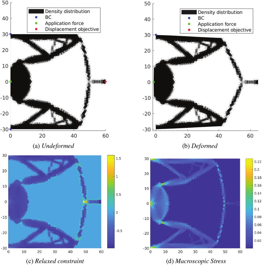
G. Capasso et al.: Mechanics & Industry 21, 304 (2020)                                 3

Algorithm 1 SIMP Algorithm                                       The chosen material is described by the potential
   Initialization:                                             density defined in [9,53] and reported in the formula
     Densities, mesh-independency filter                       below:
   Main loop:
                                                                            1                        1
     while convergence not reached do                                  Φ=     λ[log(J)]2 − µ log(J) + µ[tr(C) − 3].        (1)
        FE Analysis                                                         2                        2
        Objective and Constraints evaluation
                                                               Here J is the determinant of the deformation gradient
        Derivatives evaluation
                                                               F ; the term tr(C) denotes the trace of the right Cauchy-
        Mesh-independency filter applied to sensitivity
                                                               Green deformation tensor C = F T F ; finally,
        Update of density
        Mesh-independency filter applied to density
                                                                               E                               νE
     end while                                                         µ=                 and       λ=
   Density results analysis                                                 2(1 + ν)                     (1 − 2ν)(1 + ν)

                                                               constitute the Lamé constants of the material which are
                                                               seen as functions of Poisson ratio ν and Young Modulus
   In [51] the reader can find an exhaustive review on         E. This latter is supposed to be related to the density
numerical instabilities typical of TO. They include essen-     ρ of each element (e), through one of the two following
tially checkerboard patterns, mesh-dependencies and local      relations:
minima. To deal with the first two issues, a mesh-
independency filter can be applied [51]. A fundamental                                   Ee = ρpe E0                       (2)
aspect of such filters is the distinction between the physi-
cal densities ρ and the merely numerical ones x: the latter
category constitutes the design variable array updated in
the optimization process at each iteration; once having
updated numerical densities, these are filtered to obtain                     Ee = Emin + ρpe (E0 − Emin )                 (3)
the physical distribution of the material. NFEA is based
on physical densities ρ.                                       which will be used in order to make comparisons in our
                                                               forthcoming NFEA. Following [7], equation (2) is referred
                                                               to as calssical SIMP and equation (3) as modified SIMP.
2.2.2 Optimizer: method of moving asympthotes
When the number of design variables is very large, gra-        3.2 Nonlinear finite elements analysis
dient based optimization methods are the most efficient
algorithms. They are preferred to gradient-free optimiza-      We treat the NFEA as another minimization sub-problem
tion methods since the latter typically require many           in the global optimization: the function to minimize is
evaluations.                                                   the total energy of the system, given by both internal
   As shown in [9], the MMA is one of the most suitable        and external forces, while the constraints are the displace-
optimizers which could substitute the Optimality Criteria      ments imposed in the boundary conditions. The domain
adopted in the 88-line code by Sigmund [52], in order to       is decomposed using triangular elements.
accelerate convergence.                                           The definition of the objective function derives from
   This method is based on a local convex approxima-           the Principle of Virtual Works, where the external work
tion of objective and constraint function: this needs as       is computed as the product between the force and the
input the local evaluation of the objective function, the      displacement of the point of application:
constraints and all their derivatives with respect to the                             Z
numerical densities x.                                                     Υtot [U ] = Φ[U ]dΩ − Fext Uapp .            (4)
   The solution is said to have reached convergence when
the first order Karush Kuhn Tucker (KKT) conditions are
satisfied to an absolute tolerance of 2 × 10⁻³ .               Here, U represents the vector of the nodal displacements
                                                               which has to be determined by Variational Principle. In
                                                               order to make the Optimization Toolbox in MATLAB
3 New formulation                                              more efficient, we have to provide it with the gradient and
                                                               the Hessian of the total energy. The gradient will be the
3.1 Material description                                       residual R, computed as the difference between internal
                                                               and external forces:
A nonlinear hyperelastic material was investigated: the
same methods described in [9] were adopted, but modify-                          Def   δΥtot [U ]
ing the proposed algorithm in order to achieve the same                     R[U ] =               = Fint [U ] − Fext       (5)
                                                                                         δU
results as well as a fast convergence. Moreover, far too
little attention has been paid to the feasibility of the       where
structure itself: this can be observed by the absence of
a constraint related to the maximum stress supportable
                                                                                                Z
                                                                                                    ∂Φ[U ]
by the material.                                                                 Fint [U ] =               dΩ.             (6)
                                                                                                     ∂U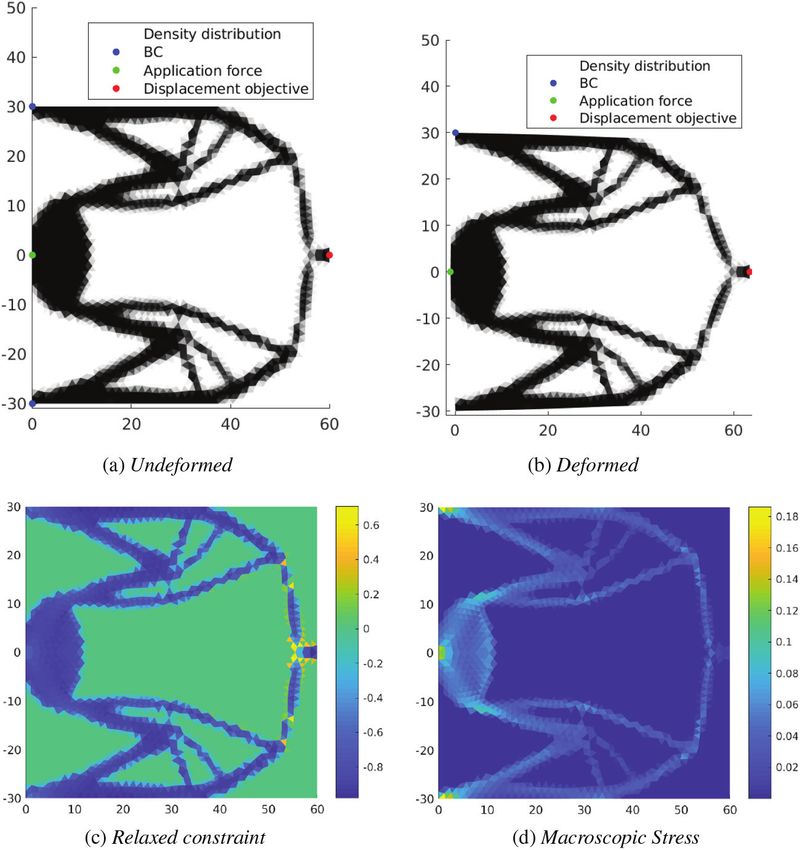
4                                             G. Capasso et al.: Mechanics & Industry 21, 304 (2020)

The Hessian will be simply the tangent stiffness matrix                where S0 is the second Piola-Kirchoff stress considering
KT , computed as the second derivative of the compliance               a material with full Young Modulus E = E0 (i.e. ρ = 1).
to the nodal displacements:                                            To access singular optima classic of mathematical program
                                                                       with vanishing constraints, a relaxation method is adopted
                                           ∂2Φ
                                      Z
                     ∂R[U ]
                    Def                                                [40]. In particular, the relaxed constraint is defined as:
           KT [U ] =        =                     dΩ.            (7)
                      ∂U T                ∂U ∂U T
                                                                                                          σ̃i
The equilibrium condition is satisfied when:                                             g i = ρ˜i            −1 ≤0                (13)
                                                                                                         σlim
                           R[UF ] = 0.                           (8)                 ρ−ρmin
                                                                       where ρ˜i = ρmax −ρmin . In classical SIMP formulation (see
The MATLAB tool fmincon is a suitable instrument to                    Eq. (2)), we have ρmin = 0.1 and ρmax = 1 while in
perform NFEA, since it treats this sub-problem as a con-               modified SIMP (see Eq. (3)) ρmin = 0 and ρmax = 1.
strained minimization problem. Moreover, it contains a
stable implementation of the Newton-Raphson Method                     3.4 Adjoint sensitivity analysis
in the Interior-Point Region [54]. This feature turns the
fmincon process into a fast and reliable solver for nonlinear          The method which is going to be illustrated has been
mechanical problems.                                                   proposed by Bhattacharyya [9]. Since the objective and
                                                                       constraint function depend both on density distribution
3.3 Stress constraint treatment                                        and nodal displacements, an adjoint sensitivity analysis
                                                                       is to be performed. In particular, we use an augmented
The Second Piola-Kirchoff stress S relates forces in the               Lagrangian L[ρ, UF (ρ)], which may be defined as follows:
reference configuration with areas also measured in the
reference configuration (see [53]). It can be calculated as
twice the derivative of the potential energy function with                                     L = f + λT R.                       (14)
respect to the right Cauchy-Green deformation tensor:
                                                                       Here f indicates a general function, indifferently the
             ∂Φ                                                        objective or the constraint; λ is a Lagrange multiplier
         S=2    = λ log(J)C −1 + µ(I − C −1 ).                   (9)   ensuring that the residual of forces R vanishes as required
             ∂C
                                                                       in equation (8). Deriving this expression and using the
The Cauchy stress, σ, which relates the forces in the                  chain rule, we obtain:
deformed configuration with areas in the deformed con-
figuration, can then be defined as:                                      dL   ∂f    ∂f dUF                     ∂R   ∂R dUF
                                                                            =    +         + λT                   +              . (15)
                                                                         dρ   ∂ρ   ∂UF dρ                      ∂ρ   ∂UF dρ
                                 1
                          σ=       F SF T .                     (10)
                                 J                                                                                     d
                                                                       Collecting all the implicit terms indicated by dρ , we
As a consequence, the microscopic (local) stress tensor                obtain:
will be evaluated as:
                                                                          dL     ∂f     T ∂R       ∂f    T ∂R     dUF
                    1                                                          =     +λ      +        +λ              . (16)
               σ=     [λ log(J)I + µ(B − I)]                    (11)       dρ    ∂ρ       ∂ρ      ∂UF      ∂UF     dρ
                    J
where B is the left Cauchy-Green tensor, which is defined              In order to eliminate the implicit dependence of free nodal
as B = F F T , and I is the second-order identity tensor.              displacements on density distribution, the lagrangian mul-
Here, microscopic stress was considered by calculating the             tiplier can be computed, remembering the definition
Von-Mises stress, under the hypothesis of plain strain. It is          of the derivative of the residual related to the nodal
important to underline the fact that this does not depend              displacements, as follows:
directly on density distribution. In this work the unified
approach proposed by Verbart et al. [40] was adopted to                                      ∂f ∂R −1     ∂f
                                                                                   λT = −             =−     K −1 .                (17)
incorporate stress constraints in topology optimization.                                    ∂UF ∂UF      ∂UF T
Assuming that the densities in SIMP represent a porous
micro-structure, one can distinguish the stress at macro-              Finally, we can obtain:
scopic (effective) versus microscopic levels [55]. The former
is the stress computed using the Young modulus of the                                       dL   ∂f      ∂R
SIMP model (c.f. Eqs. (2)–(3). The latter is computed                                          =    + λT    .                      (18)
                                                                                            dρ   ∂ρ      ∂ρ
considering a stress model that mimics the behavior of
the “local stress” in a rank-2 layered composite [55]. For
this reason we identify the microscopic stress as:                     One can observe that the evaluation of gradients only
                                                                       requires a linear system of equation resolution, extremely
                                 1                                     convenient if compared with direct or finite difference
                          σ̃ =     F S0 F T                     (12)   approaches.
                                 J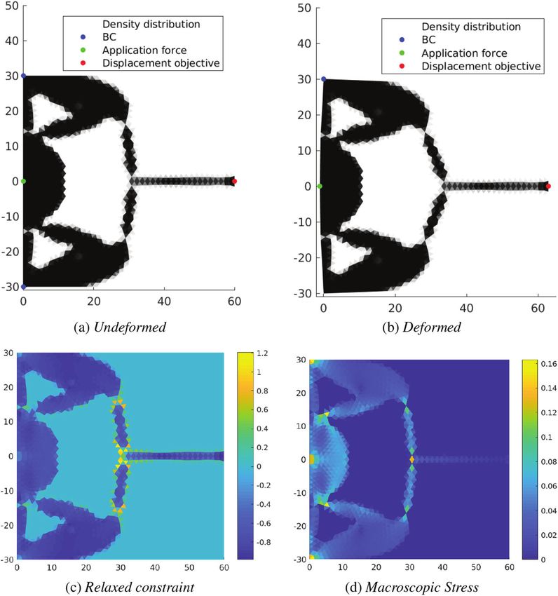
G. Capasso et al.: Mechanics & Industry 21, 304 (2020) 5
3.5 Density filtering
As pointed out in Section 2.2, a mesh-independency filter
was applied to deal with certain numerical instabili-
ties, namely checkerboard patterns and mesh-dependent
solutions [51].
Here the method suggested by Bruns and Tortorelli [56]
was implemented, where:
P
wij xi
ρj = Pi . (19)
i wij
Here wij is the weight associated with the ith ele-
ment within the prescribed neighborhood of the jth one,
determined as: Fig. 1. Initial domain: airfoil optimization problem.
wij = max(0, Rmin − rij ). (20) Using the classical SIMP approach (see Eq. (2)), the
whole problem can be formalized as follows:
The parameter Rmin , called filter radius, is the radius of
the specified neighborhood and rij the distance between
min0.1≤ρ≤1 V
the centroids of the two elements. This formulation pro-
s.t. U e ≤ U0 (22)
posed in [56] is valid under the assumption of uniform
σi ≤ σlim ∀i = 1, . . . , N.
mesh. This filter makes the results independent from
the adopted mesh, improving the resolution as Rmin
decreases. However, the maximal resolution is linked to Here V represents the volume fraction, Ue the displace-
the mesh itself, since the minimum applicable value Rmin ment at the trailing edge and σlim is the highest tolerable
cannot be smaller than the size of the largest element. stress in the structure (to avoid failure). The constraint
When computing derivatives with respect to the numer- relative to the σ in each element is due to the desire to
ical densities x (necessary to gradient-based optimization design a feasible structure while not reaching the weakest
methods), two steps are followed: firstly, derivatives with one: in particular, we will consider the Von-Mises stress,
respect to physical densities ρ have to be computed; then, under the hypothesis of plain strain. Finally, the con-
chain rule is applied to obtain the desired gradient. straint on Ue derives from the necessity of designing an
efficient shape morphing wing.
We shall also perform further analyses based on the
3.6 Constraint aggregation modified SIMP approach (see Eq. (3)), for comparisons.
The new optimization problem is then:
Treating the relaxed stress distribution, there would be an
excess of constraints. So the maximum may be taken into
account to represent the whole domain. Given the fact min0≤ρ≤1 V
s.t. Ue ≤ U0
that the max function is non-derivable, the lower bound (23)
Kreisselmeier-Steinhauser function [36,57] was employed:
σi ≤ σlim ∀i = 1, . . . , N
C ≥ Cmin .
N
!
1 1 X P gi
max gi ≈ GlKS = log e . (21) Here another constraint has to be added, since the vol-
i P N i=1 ume fraction minimization under stress constraint, would
generate gray regions, preventing the creation of a con-
The larger the factor P , the better the approximation tinuous chain between force application point and trailing
of the max, but also the more expensive the computa- edge. Such constraint will be an inferior limit on the com-
tional cost of the overall optimization process. In fact the pliance C of the trailing edge region [35]: this value is
non-linearity of the optimization problem is enhanced by arbitrarily defined as the initial compliance.
the use of higher values of P . Therefore, P has to be cho-
sen as an appropriate compromise between computational 4.2 Second optimization problem: geometric inverter
burden and accuracy in stress control.
The second optimization problem is a more realistic test
case, inspired by the work in [35]. Figure 2 illustrates the
4 Applications initial domain.
The idea is to design a compliant mechanism which
4.1 First optimization problem: NACA airfoil would invert the input displacement, creating as output
another displacement on the opposite side of the structure.
As an academic example, this part focuses on the The actual input is a force. The optimized mechanism
minimization of the weight of a shape morphing wing. is defined as the one capable of reaching the highest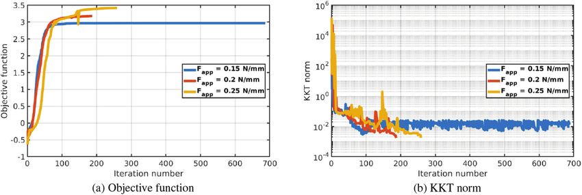
6 G. Capasso et al.: Mechanics & Industry 21, 304 (2020)
Table 1. Default parameters used in the Airfoil optimiza-
tion problem.
Number of design variables 2065
Number of nodes 1136
Number of degrees of freedom 2152
Young Modulus E0 [MPa] 15
Minimum Young Modulus Emin [MPa] 0.015
Poisson ratio ν 0.3
Lamé first parameter λ0 [MPa] 8.65
Lamé second parameter µ0 [MPa] 5.77
Minimum Lamé first parameter λmin [MPa] 0.00865
Minimum Lamé second parameter µmin [MPa] 0.00577
Displacement constraint U0 [mm] −21
Stress constraint σlim [MPa] 1
Chord length c [mm] 150
Abscissa force’s application point xapp /c 0.3
Ordinate force’s application point yapp [mm] 5
Intensity applied force Fext [N/mm] 7
Fig. 2. Geometric inverter scheme. Limits of Boundary Conditions x/c [%] 35 − 65
Penalization factor p 3.0
Radius filter Rmin [mm] 6.0
ratio between output and input; as the two displacements Aggregation constant P 4
have opposite signs, this is translated into a minimization
problem:
The advantage of our methodology is that stress dis-
min0≤ρ≤1 Uout /Uin tribution is already computed in our optimization loop
s.t. V ≤ V0 (“Constraints evaluation” in Algorithm 1).
(24)
σi ≤ σlim ∀i = 1, . . . , N
C ≥ Cmin . 5.1 NACA airfoil
The second pseudo-density parameterization of the SIMP A first analysis is performed on the two problems 22 and
Algorithm is adopted. Before the main loop, the topol- 23, considering the same domain (represented in Fig. 1).
ogy is initialized by imposing ρ = V0 in every element of The parameters adopted in this section are reported in
the domain. The constraints are quite similar to the ones Table 1.
adopted in the previous section. We have thus:
5.1.1 First formulation results
– volume fraction: the structure has to be as light as
possible, to reduce costs and weight; In this subsection, the results to the problem (22) are pre-
– stress: the whole mechanism has to support the sented. The base structure can be observed in Figure 3a.
applied load without breaking, or reaching the yield This can be decomposed into four main sectors:
point;
– compliance: a continuous chain between input and – Front sector: This is responsible for stress redistribu-
output is ensured, by imposing that the output tion, as illustrated in Figure 3d. The stresses use this
region has to keep the same compliance at the first path in order to create an equilibrating moment. The
iteration loop (where ρ = V0 in every finite element) middle part, situated between the front chain and
[35]. the application point of the external force, is empty:
in fact, the volume fraction constrained minimiza-
Another aspect which appeared fundamental is the sym- tion produces this result, where the stresses have to
metric nature of the domain: to accelerate computation, be collocated in an intermediate location. Moreover,
only half of the whole domain has been simulated. this sector connects the two series of points where
the homogeneous Boundary Conditions are applied.
– Central chain: This sector is the transmitter of forces
5 Results and discussion between the application point of the external force
and the rear chain (discussed later), as shown in
In this section, numerical results are presented and dis- the macroscopic stress distribution (Fig. 3d). It is
cussed. Simulations have been performed using a unique directly linked to all the other parts of the optimized
MATLAB code, adopting the original MMA code pro- structure.
vided by Svanberg [52] and without altering its default – Inferior chain: It is the main link between the central
parameters. Given the fact that the constraint is approxi- chain and the inferior BCs. In the base structure, It
mated (as explained in Sects. 3.3 and 3.6) stress distribu- is also directly linked to the front part: this is due to
tion post-processing on the optimal structure is necessary. the fact that it starts exactly at the left limit of the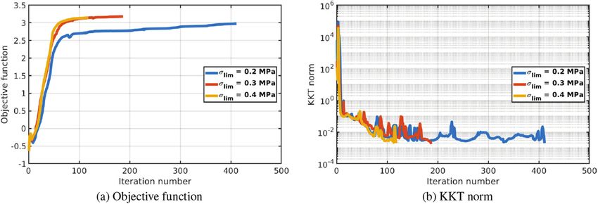
G. Capasso et al.: Mechanics & Industry 21, 304 (2020) 7
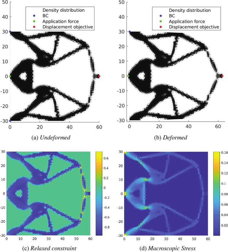
Fig. 3. Results relative to the Airfoil problem (first formulation).
inferior boundary points affected by the application The differences are evident by comparing Figure 3 and
of homogeneous BCs. Figure 4.
– Rear chain: This is the only part not interested in As was visible in the previous numerical experiment, the
any redistribution of stresses, as shown in Figure 3c aggregation method does not always guarantee the respect
and d. Its main role is transmitting the commanded of the stress limits: this is a consequence of the GKS
displacement at the trailing edge, thanks to an input approximation. This time, an overshoot can be found on
force provided by the central chain. This sector the filled structure. A lower limit on the stress should have
affects the volume fraction negatively, given that it been introduced in order to adapt to the real constraint.
doesn’t have to carry any stress. The logic behind the optimal structure presented in
Figure 4 (solution of the problem (22)) is unaltered com-
The optimized structure in deformed configuration is pared with to the first one in Figure 3 (solution of the
illustrated in Figure 3b. The reader can observe the logic problem (23)).
at the base of the mechanism. By introducing a single However, this formulation leads to a more efficient
input force at the node in green, the effort is transmitted application of the stress constraint, since all empty
to the rear chain through the central sector. Simultane- elements do not contribute to the macroscopic stress dis-
ously, the inferior chain and the front sector connect the tribution. An immediate consideration is the removal of
central chain to the nodes in blue (where homogeneous most of the Front sector and the Rear chain from the pre-
Dirichlet Boundary Conditions are applied). Finally, the vious results: globally the obtained volume fraction would
rear chain converts the input force into a displacement at be inferior.
the trailing edge. As a consequence, the modified SIMP approach (see
The distribution of the relaxed constraint proves the Eq. (3)) is more suitable for topology optimization prob-
approximated nature of the GKS function: this is not lems presenting a stress constraint. This consideration is
always guaranteed, but it is the product of a compro- applied in the second part of the present work.
mise between precision, stability and computational cost.
However, the only elements where the relaxed constraints 5.2 Geometric inverter
are not satisfied are, effectively, “empty”.
Out of the previous academic examples, the second formu-
5.1.2 Second formulation results lation has been identified as a better compromise between
severity of the penalization on stress constraint and real-
When using the second formulation to parameterize the ity of the final structure, leading to a much lighter final
topology, a totally different structure is obtained. Results structure. However, a lower limit on the stress has to be
from problem (23) are presented in this subsection. introduced.
8                                     G. Capasso et al.: Mechanics & Industry 21, 304 (2020)

                             Fig. 4. Results relative to the Airfoil problem (second formulation).

Table 2. Default parameters used in the Inverter opti-              – Central Bulb: It absorbs the applied force and
mization problem (symmetrical problem).                               transmits it to the rest of the structure.
    Number of design variables                      2464            – Support Net: It guarantees an efficient redistribution
    Number of nodes                                 1293              of stresses all over the structure: the ramifications
    Number of degrees of freedom                    2543              create the necessary moments to equilibrate the
    Young Modulus E0 [MPa]                          11                whole mechanism. In fact, as the available vol-
    Minimum Young Modulus Emin [MPa]                0.011             ume fraction constrained, the resulting positioning
    Poisson ratio ν                                 0.4               produces the best compromise.
    Lamé’s first parameter λ0 [MPa]                15.71           – Angular chain: This connects the Support Net with
    Lamé’s second parameter µ0 [MPa]               3.93              the clamped point, guaranteeing the force equilib-
    Minimum Lamé’s first parameter λmin [MPa]      0.01571           rium of the structure.
    Minimum Lamé’s second parameter µmin [MPa]     0.00393         – Terminal chain: It make the morphing nature of the
    Stress constraint σlim [MPa]                    0.3               whole mechanism possible, generating the displace-
    Domain width c [mm]                             60                ment in output.
    Domain height c [mm]                            60
    Intensity applied force Fext [N/mm]             0.2            The relaxed stress constraint and macroscopic stress
    Penalization factor p                           3.0          distributions present some differences: in fact, the former
    Radius filter Rmin [mm]                         1.25         reports a stress constraint violation in the elements of
    Aggregation constant P                          4            the terminal chain of the actuator, where the displace-
                                                                 ments are higher, due to the aggregation; this violation
                                                                 disappears in the macroscopic stress distribution. On the
                                                                 contrary, the maximum effective stress is in the areas of
  In the second test case of the present article, modified       higher curvature.
SIMP was adopted. Moreover, only half of the domain
has been considered in the simulation to accelerate com-
                                                                 5.2.1 Influence of stress constraint
putation (symmetric properties have been exploited). All
the parameters characterizing the Inverter problem are           Further numerical analyses were performed, in order to
reported in Table 2.                                             investigate the effects of the stress constraint. In particu-
  In Figure 5 the final structure is presented. In the           lar, both increases and decreases on the stress limits were
deformed configuration (Fig. 5b), the gain in terms of           considered.
displacement inversion is easily visible.                           If the stress limit decreases to 0.2 MPa, the obtained
  Each half of the compliant mechanism can be decom-             structure is totally altered (results reported in Fig. 6).
posed into four main sectors:                                    However, the global decomposition follows the same logic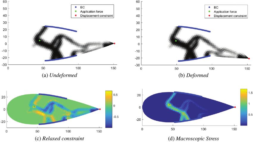
G. Capasso et al.: Mechanics & Industry 21, 304 (2020)                               9

                                      Fig. 5. Results relative to the Inverter problem.

adopted in the previous section. Four main differences          Table 3. Numerical results of the Inverter optimization
may be noticed:                                                 problem (24) with variations in σlim .
                                                                            σlim [MPa]    Objective   N. iterations
   – the Central Bulb is more compact and does not
     present any hole;                                                      0.2           2.9807      411
                                                                            0.3           3.1823      187
   – the Support Net presents only two ramifications;
                                                                            0.4           3.1455      118
   – the Angular Chain and the Support Net cannot be
     distinguished;
   – the Terminal Chain is much longer than before.               In Table 3 the numerical results are shown for each
                                                                value of σlim . In particular, it has been demonstrated that
   The reader can easily understand the necessity of intro-     higher limit in terms of allowed stress doesn’t necessarily
ducing an additional buckling constraint if the stress limit    imply an augmentation in final performances. Moreover,
is exaggeratedly low.                                           the number of iterations to convergence augments as σlim
   An analogue analysis was performed for an augmented          decreases.
allowed limit stress of the material (results reported in
Fig. 7). The differences are less evident than an analogue
                                                                5.2.2 Influence of the amplitude of the applied load
reduction on stress limits. However, the Support Net is
more ramified, allowing for a different allocation of the       The applied load shows little differences with respect to
efforts.                                                        the base structure. In particular, the Support Net is less
   Another fundamental aspect is the imperfect exploita-        ramified for higher loads : this reflects again the same
tion of the material: in fact, the stress constraint isn’t      effect of a very small reduction in acceptable limit stress.
active, leading to a structure where the maximum macro-            Moreover, as the amplitude of the force increases,
scopic stress isn’t reached (refer to Fig. 7d).                 an evident overshoot on the macroscopic stress can be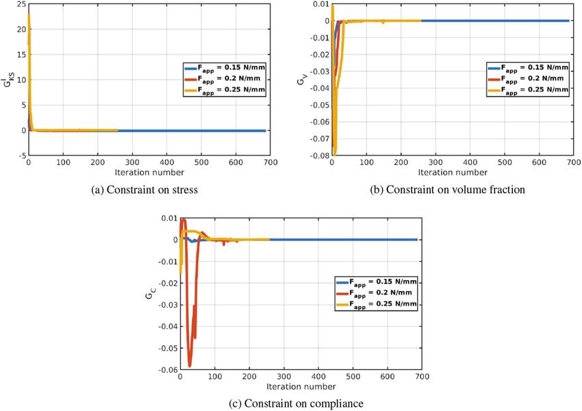
10                                   G. Capasso et al.: Mechanics & Industry 21, 304 (2020)

                              Fig. 6. Results relative to the inverter problem (σ = 0.2 MPa).

Table 4. Numerical results of the Inverter optimization        geometric inverter. A continuous material distribution
problem (24) with variations in Fapp .                         problem following the SIMP approach was formulated
          Fapp [N/mm]    Objective   N. iterations             to find the optimal layout throughout a design domain.
                                                               For our purpose, a hyperelastic Neo-hookean material was
          0.15           2.9684      687                       chosen.
          0.20           3.1823      187                          We considered two TO problems. The first one con-
          0.25           3.4236      259
                                                               sists in the minimization of the volume fraction of a
                                                               NACA 0033 airfoil, which must be conceived as capa-
observed: this leads to the idea that another approxima-       ble of reaching a fixed displacement at its trailing edge.
tion for the max is needed.                                    The second TO problem aims at maximizing the geomet-
   In the Appendix, different designs of the optimized         ric gain in a structure with given volume fraction, in order
structure are presented.                                       to design a geometric inverter starting from a rectangular
   In Table 4 the numerical results are presented for each     initial domain. The stress distribution was considered as
value of Fapp . By increasing the amplitude of the applied     the main constraint in all the problems presented in this
load, the geometric advantage improves: however, the gain      paper. In particular, a relaxation and aggregation method
isn’t proportional to the relative augmentation in terms of    was adopted to treat this constraint optimally.
applied force. On the other hand, a general rule governing        The problem of morphing wing design was solved using
the number of iterations cannot be exploited.                  two different models of the relation between Young Mod-
                                                               ulus E and density ρ of each element, namely classical
6 Conclusion                                                   SIMP and modified SIMP (see Eqs. (2)–(3)). The objec-
                                                               tive is always to minimize the volume fraction V , under
Topology Optimization was used to design two differ-           constraints of performance (in terms of trailing edge dis-
ent compliant mechanisms: a morphing wing and a                placement) and of feasibility (in terms of stress). Results
G. Capasso et al.: Mechanics & Industry 21, 304 (2020) 11
Fig. 7. Results relative to the inverter problem (σ = 0.4 MPa).
showed a substantial gain in terms of V when we adopted The position of the input force was considered as an
the modified SIMP rather than classical SIMP: we pass input of each optimization problem presented in this
from a volume fraction of 51.64% to 19.62%. The second paper, but could be treated as a new design variable as
structure is also easier to manufacture using a 3-D print- well.
ing technique or additive manufacturing, which are the Moreover, the two optimization problems could be
natural outputs of Topology Optimization. extended to 3D analysis, allowing also the introduction
Modified SIMP approach was applied to parameterize of more realistic Boundary Conditions.
the domain in the geometric inverter problem. The first Future works will focus on the application of stress-
results show a ratio of 318% between output and input based TO on the design of a morphing winglet subject to
displacement (respectively Uout and Uin in Fig. 2). Several very high deformations.
analyses were performed, by modifying the stress limits Looking forward, further attempts with different opti-
or the applied load. One can observe that increasing the mization problems could prove beneficial to literature on
stress constraint does not imply a significant gain in terms the subject.
of structure performances. By analyzing the effects of the
applied load, the geometric gain increases as the force
increases, but the relation is not linear.
Looking at the number of iterations, by reducing the References
allowed stress, convergence results to be slower; on the
other hand, a general dependence between number of [1] M.P. Bendsøe, N. Kikuchi, Generating optimal topologies in
iterations and applied load cannot be proved. structural design using a homogenization method, Comput.
Globally, the present work demonstrated how a light Methods Appl. Mech. Eng. 71, 197–224 (1988)
structure can be easily designed through TO even with [2] M.P. Bendsøe, O. Sigmund, Material interpolation schemes
hyperelastic material responses and stress constraints. in topology optimization, Arch. Appl. Mech. 69, 635–654
Nonlinear stress constraints were treated trough aggrega- (1999)
tion based on the lower bound Kreisselmeier-Steinhauser [3] M. Zhou, G. Rozvany, The COC algorithm, Part II: topo-
function: effects of different aggregation functions could logical, geometrical and generalized shape optimization,
be further investigated. Comp. Methods Appl. Mech. Eng. 89, 309–336 (1991)12 G. Capasso et al.: Mechanics & Industry 21, 304 (2020)
[4] Y.M. Xie, G.P. Steven, A simple evolutionary procedure [22] H.C. Gea, J. Luo, Topology optimization of structures with
for structural optimization, Comput. Struct. 49, 885–896 geometrical nonlinearities, Comput. Struct. 79, 1977–1985
(1993) (2001)
[5] G. Allaire, F. Jouve, A.M. Toader, Structural optimiza- [23] S.M. Han, S.I. Kim, Y.Y. Kim, Topology optimization of
tion using sensitivity analysis and a level-set method, J. planar linkage mechanisms for path generation without pre-
Comput. Phys. 194, 363–393 (2004) scribed timing, Struct. Multidiscipl. Optim. 56, 501–517
[6] M.Y. Wang, X. Wang, D. Guo, A level set method for struc- (2017)
tural topology optimization, Comput. Methods Appl. Mech. [24] C.B.W. Pedersen, T. Buhl, O. Sigmund, Topology synthesis
Eng. 192, 227–246 (2003) of large-displacement compliant mechanisms, Int. J. Numer.
[7] E. Andreassen, A. Clausen, M. Schevenels, B.S. Lazarov, Methods Eng. 50, 2683–2705 (2001)
O. Sigmund, Efficient topology optimization in MATLAB [25] M.P. Bendsøe, J.M. Guedes, S. Plaxton, J.E. Taylor, Opti-
using 88 lines of code, Struct. Multidiscip. Optim. 43, 1–16 mization of structure & material properties for solids
(2010) composed of softening material, in IUTAM Symposium on
[8] O. Sigmund, A 99 line topology optimization code writ- Optimization of Mechanical Systems. Springer, Netherlands
ten in Matlab, Struct. Multidiscipl. Optim. 21, 120–127 (1996), pp. 17–24
(2001) [26] M. Bogomolny, O. Amir, Conceptual design of reinforced
[9] A. Bhattacharyya, C. Conlan-Smith, K.A. James, Topol- concrete structures using topology optimization with elasto-
ogy optimization of a bi-stable airfoil using nonlinear plastic material modeling, Int. J. Numer. Methods En. 90,
elasticity. In: 18th AIAA/ISSMO Multidisciplinary Anal- 1578–1597 (2012)
ysis and Optimization Conference. American Institute of [27] K. Maute, S. Schwarz, E. Ramm, Adaptive topology opti-
Aeronautics and Astronautics (2017) mization of elastoplastic structures, Struct. Optim. 15,
[10] G. Capasso, R. Amargier, S. Coniglio, J. Morlier, C. Mabru, 81–91 (1998)
M. Di Sciuva, Structural optimization for propulsion [28] G.H. Yoon, Y.Y. Kim, Topology optimization of material-
aiframe, M.Sc. thesis, Politecnico di Torino, 2019 nonlinear continuum structures by the element connectivity
[11] G. Capasso, S. Coniglio, M. Charlotte, J. Morlier, Opti- parameterization, Int. J. Numer. Methods Eng. 69, 2196–
misation topologique de structures adaptatives (bi-stables) 2218 (2007)
en mécanique non-linéaire, in 14éme Colloque National en [29] K. Yuge, N. Iwai, N. Kikuchi, Optimization of 2-d
Calcul des Structures (2019) structures subjected to nonlinear deformations using the
[12] S. Coniglio, C. Gogu, R. Amargier, J. Morlier, Pylon homogenization method, Struct. Optim. 17, 286–299 (1999)
and engine mounts performance driven structural topology [30] K. Yuge, N. Kikuchi, Optimization of a frame structure
optimization, in World Congress of Structural and Multi- subjected to a plastic deformation, Struct. Optim. 10, 197–
disciplinary Optimisation. Springer (2017), pp. 1349–1363 208 (1995)
[13] J.H. Zhu, W.H. Zhang, L. Xia, Topology optimization in [31] X. Huang, Y. Xie, Topology optimization of nonlinear
aircraft and aerospace structures design, Arch. Comput. structures under displacement loading, Eng. Struct. 30,
Methods Eng. 23, 595–622 (2016) 2057–2068 (2008)
[14] P. Bettini, A. Airoldi, G. Sala, L.D. Landro, M. Ruzzene, A. [32] X. Huang, Y.M. Xie, G. Lu, Topology optimization of
Spadoni, Composite chiral structures for morphing airfoils: energy-absorbing structures, Int. J. Crashworthiness 12,
numerical analyses and development of a manufacturing 663–675 (2007)
process. Compos. Part B: Eng. 41, 133–147 (2010) [33] D. Jung, H.C. Gea, Topology optimization of nonlin-
[15] P.R. Budarapu, Y.B. Sudhir Sastry, R. Natarajan, Design ear structures, Finite Elem. Anal. Des. 40, 1417–1427
concepts of an aircraft wing: composite and morphing airfoil (2004)
with auxetic structures, Front. Struct. Civil Eng. 10, 394– [34] M.J. Werkheiser, J. Dunn, M.P. Snyder, J. Edmunson, K.
408 (2016) Cooper, M.M. Johnston, 3d printing in zero-g ISS tech-
[16] K.C.W. Cheung, Digital cellular solids : reconfigurable com- nology demonstration, in AIAA SPACE 2014 Conference
posite materials. PhD thesis, Massachusetts Institute of and Exposition. American Institute of Aeronautics and
Technology (2012) Astronautics (2014)
[17] A. Airoldi, M. Crespi, G. Quaranti, G. Sala, Design of a [35] C. Conlan-Smith, A. Bhattacharyya, K.A. James, Optimal
morphing airfoil with composite chiral structure, J. Aircraft design of compliant mechanisms using functionally graded
49, 1008–1019 (2012) materials, Struct. Multidiscipl. Optim. 57, 197–212 (2017)
[18] S. Joshi, Z. Tidwell, W. Crossley, S. Ramakrishnan, Com- [36] R. Yang, C. Chen, Stress-based topology optimization,
parison of morphing wing stategies based upon aircraft per- Struct. Optim. 12, 98–105 (1996)
formance impacts, in 45th AIAA/ASME/ASCE/AHS/ASC [37] G. Da Silva, E. Cardoso, Stress-based topology optimiza-
Structures, Structural Dynamics Materials Conference. tion of continuum structures under uncertainties, Comp.
American Institute of Aeronautics and Astronautics (2004) Methods Appl. Mech. Eng. 313, 647–672 (2017)
[19] J.M. Martinez, D. Scopelliti, C. Bil, R. Carrese, P. [38] C. Kiyono, S. Vatanabe, E. Silva, J. Reddy, A new multi-
Marzocca, E. Cestino, G. Frulla, Design, analysis and exper- p-norm formulation approach for stress-based topology
imental testing of a morphing wing, in 25th AIAA/AHS optimization design. Comp. Struct. 156, 10–19 (2016)
Adaptive Structures Conference. American Institute of [39] S.J. Moon, G.H. Yoon, A newly developed QP-relaxation
Aeronautics and Astronautics (2017) method for element connectivity parameterization to
[20] D. Wagg, I.P.W. Bond, M. Friswell, Adaptive structures – achieve stress-based topology optimization for geometri-
engineering applications (2007) cally nonlinear structures, Comp. Methods Appl. Mech.
[21] T. Buhl, C. Pedersen, O. Sigmund, Stiffness design of Eng. 265, 226–241 (2013)
geometrically nonlinear structures using topology optimiza- [40] A. Verbart, M. Langelaar, F. van Keulen, A unified
tion, Struct. Multidiscip. Optim. 19, 93–104 (2000) aggregation and relaxation approach for stress-constrainedG. Capasso et al.: Mechanics & Industry 21, 304 (2020) 13
topology optimization, Struct. Multidiscipl. Optim. 55, [49] M. Zhou, G. Rozvany, The COC algorithm, Part II: Topo-
663–679 (2016) logical, geometrical and generalized shape optimization,
[41] C. Le, J. Norato, T. Bruns, C. Ha, D. Tortorelli, Stress- Comp. Methods Appl. Mech. Eng. 89, 309–336 (1991)
based topology optimization for continua, Struct. Multidis- [50] T. Bruns, A reevaluation of the simp method with filter-
cipl. Optim. 41, 605–620 (2010) ing and an alternative formulation for solid–void topology
[42] M. Bruggi, P. Duysinx, Topology optimization for mini- optimization, Struct. Multidiscip. Optim. 30, 428–436
mum weight with compliance and stress constraints. Struct. (2005)
Multidiscipl. Optim. 46, 369–384 (2012) [51] O. Sigmund, J. Petersson, Numerical instabilities in
[43] N.H. Kim, Introduction to Nonlinear Finite Element Anal- topology optimization: a survey on procedures dealing
ysis. Springer US (2014) with checkerboards, mesh-dependencies and local minima,
[44] S. Coniglio, J. Morlier, C. Gogu, R. Amargier, Generalized Struct. Optim. 16, 68–75 (1998)
geometry projection: a unified approach for geometric fea- [52] K. Svanberg, The method of moving asymptotes|a new
ture based topology optimization, Arch. Comput. Methods method for structural optimization, Int. J. Numer. Methods
Eng. 1–38 (2019) Eng. 24, 359–373 (1987)
[45] W. Zhang, W. Yang, J. Zhou, D. Li, X. Guo, Structural [53] R.W. Ogden, Non-Linear Elastic Deformations. Courier
topology optimization through explicit boundary evolution, Corporation (2013)
J. Appl. Mech. 84, 011011 (2016) [54] P.Y. Papalambros, D.J. Wilde, Principles of Optimal
[46] W. Zhang, J. Yuan, J. Zhang, X. Guo, A new topology opti- Design. Cambridge University Press (2000)
mization approach based on moving morphable components [55] P. Duysinx, M.P. Bendsøe, Topology optimization of contin-
(MMC) and the ersatz material model, Struct. Multidiscipl. uum structures with local stress constraints, Int. J. Numer.
Optim. 53, 1243–1260 (2015) Methods Eng. 43, 1453–1478 (1998)
[47] G.I. Rozvany, Aims, scope, methods, history and uni- [56] T. Bruns, D. Tortorelli, Topology optimization of non-linear
fied terminology of computer-aided topology optimization elastic structures and compliant mechanisms. Comput.
in structural mechanics, Struct. Multidiscip. Optim. 21, Methods Appl. Mech. Eng. 190, 3443–3459 (2001)
90–108 (2001) [57] G. Kreisselmeier, R. Steinhauser, Systematic control design
[48] G.I. Rozvany, M. Zhou, T. Birker, Generalized shape by optimizing a vector performance index, in Computer
optimization without homogenization, Struct. Optim. 4, aided design of control systems. Elsevier (1980), pp. 113–
250–252 (1992) 117
Cite this article as: G. Capasso, J. Morlier, M. Charlotte, S. Coniglio, Stress-based topology optimization of compliant
mechanisms using nonlinear mechanics, Mechanics & Industry 21, 304 (2020)14 G. Capasso et al.: Mechanics & Industry 21, 304 (2020)
Appendix A
Fig. A.1. Results relative to the inverter problem: applied force Fapp = 0.15 N/mm.G. Capasso et al.: Mechanics & Industry 21, 304 (2020) 15
Fig. A.2. Results relative to the inverter problem: Variation of the applied force Fapp = 0.25 N/mm.
Fig. A.3. Convergence curves for problem (24): variations in σlim .16 G. Capasso et al.: Mechanics & Industry 21, 304 (2020)
Fig. A.4. Evolution of optimization constraints (expressed in negative null form) for problem (24): variations in σlim .
Fig. A.5. Convergence curves for problem (24): variations in Fapp .G. Capasso et al.: Mechanics & Industry 21, 304 (2020) 17 Fig. A.6. Evolution of optimization constraints (expressed in negative null form) for problem (24): variations in Fapp .
You can also read