Supplementary Materials for - Science
←
→
Page content transcription
If your browser does not render page correctly, please read the page content below
Supplementary Materials for
Estimating infectiousness throughout SARS-CoV-2 infection course

 Terry C. Jones1,2,3†, Guido Biele4,5†, Barbara Mühlemann1,2, Talitha Veith1,2, Julia Schneider1,2,
  Jörn Beheim-Schwarzbach1, Tobias Bleicker1, Julia Tesch1, Marie Luisa Schmidt1, Leif Erik
 Sander6, Florian Kurth6,7, Peter Menzel8, Rolf Schwarzer8, Marta Zuchowski8, Jörg Hofmann8,
     Andi Krumbholz9,10, Angela Stein8, Anke Edelmann8, Victor Max Corman1,2, Christian
                                             Drosten1,2*

                        Correspondence to: christian.drosten@charite.de

This PDF file includes:

       Supplementary Text
       Figs. S1 to S17
       Tables S1 to S5

                                                                                                      1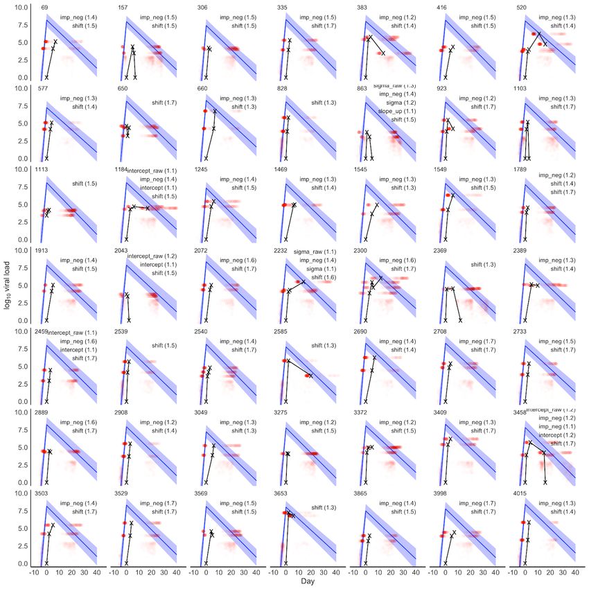
Supplementary Text

Per-subject day of detection and peak viral load
First-positive samples may be obtained at different time points in the course of the infections of
different individuals. Comparisons of viral loads from uncertain infection time points may
therefore be misleading. Even when reliably known, differences or lack of differences in first-
positive viral loads may not be present at other time points in the course of infections. These
important concerns are even more pressing in a dataset containing subjects who were PAMS at
the time of detection, because the time range of their samples will be broader, and possibly
include the period of virus increase. Our mean estimated time of infection detection of 7.30
(7.11, 7.50) days after peak viral load with standard deviation of 7.68 (7.58, 7.77) days makes it
clear that the first-positive viral loads in our dataset are derived from samples spanning a broad
infection time range. It must be remembered that Figs. 2A, 2B, 2D, 2E, 2F and the
horizontal/vertical lines in Fig. 2C are all based on viral loads from the first positive test and that
differences or similarities at time of detection might not be present at other time points.

We cannot use results from the time series analysis to answer questions regarding temporal
differences between PAMS and Hospitalized subjects. This is because we do not have sufficient
time series data to determine with certainty whether the peak viral load of PAMS subjects differs
from that of Hospitalized subjects as it does in the first-positive tests. A first-positive viral load
difference due to time of detection is quite plausible since PAMS subjects are likely to be
detected earlier when contact tracing is used, and younger PAMS subjects are likely detected
earlier in community and employee testing. On the other hand, symptomatic cases are often
detected by doctors, with the patients only later referred to Charité – Universitätsmedizin for
further tests, possibly resulting in later first-positive RT-PCR tests in our dataset. PAMS subjects
over age 70 are less likely to present at test centers, so may be detected later than symptomatic
elders, with lower first-positive viral loads, as in Fig. 2A.

Time to peak viral load
Our estimate of 4.31 (4.04, 4.60) days from onset of shedding to peak viral load is similar to the
upper bounds of those in a non-symptoms-driven study of basketball players, including 35
subjects with a leading negative test often obtained within two days of the first positive test (18).
There, the time from a negative test to peak viral load was estimated at 2.9 days (95% CI: 0.7,
4.7) for symptomatic and 3.0 days (1.3, 4.3) for asymptomatic subjects. These estimates of time
to peak viral load can be considered vis-à-vis estimates of incubation time of 4.8-6.7 days from
studies of symptomatic patients (4, 39–43). If these estimates are reasonably accurate, the time
difference suggests that peak viral load occurs 1-3 days before symptom onset, in accordance
with other studies (41, 98). Also of note, our 1.8 (1.3, 2.6) day estimate of the time from
undetectable to peak infectiousness is similar to the 1.5 day period of rise in pre-symptomatic
shedding calculated by Lau et al. (99).

                                                                                                      2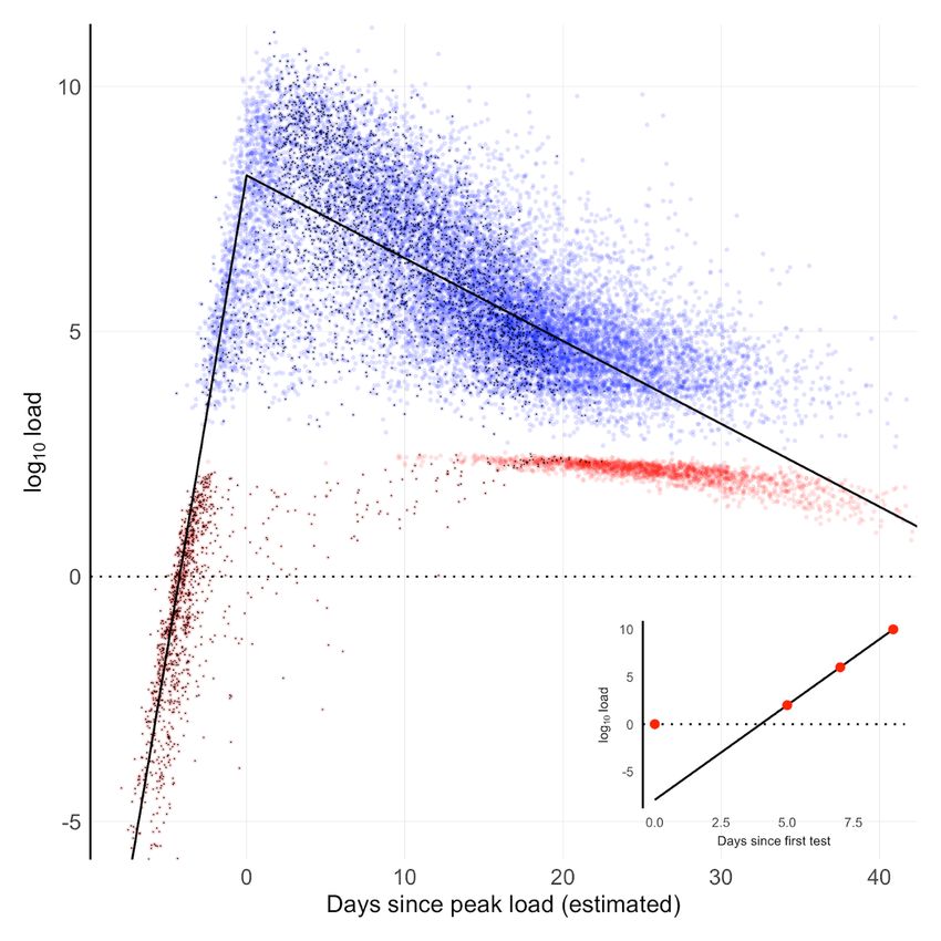
Viral load decline over time
Our estimate of the viral load decline slope of -0.17 overlaps the lower end of the -0.15 (95% CI:
-0.19 to -0.11) range of one study (74) and is steeper than other estimates, spanning -0.15 to -
0.06 (41, 100). This could be because our data is from the full time course of infections,
incorporating information from estimated day of infection and peak viral load, and we have
many subjects with multiple tests who were never hospitalized, whereas the other studies involve
symptomatic hospitalized patients. A ballpark calculation suggests that our estimate is
reasonable. Successful culture isolation has not been achieved beyond 9-10 days after symptom
onset (19, 20, 35, 45, 46) in non-severe cases, with viral load falling to somewhere between 5.4
and 6.6 log10 RNA copies by that time (19, 20, 63). We estimate a mean peak viral load of 8.1
(8.0, 8.3), so a viral load decline from that peak range to 6.0 at our mean slope would take 11.8
to 13.5 days. This suggests peak viral load occurs roughly 1-3 days prior to onset of symptoms,
matching the estimate above. The rate of viral load decline is likely influenced by disease
severity, treatment, comorbidities, and patient immune status, with no simple causation, as
suggested by reports of slower decline of viral load in mild infections (1) but also prolonged
elevated viral load time courses of critical or severe hospitalized cases (63, 101, 102).

Onset of symptoms data from a hospitalized cohort
We examined patient-estimated day of onset of symptoms reported by a Charité –
Universitätsmedizin cohort of 171 hospitalized patients (76, 77) for whom RT-PCR time series
data was also available. These data suggest a time from peak viral load to onset of symptoms of
4.3 days, higher than the two 1-3 day ballpark estimates above. However, it must be remembered
that this is a small, entirely hospitalized cohort, and that patient recall of the day of symptom
onset is not fully reliable, so the 4.3 day figure must also be considered approximate. The
posterior distribution of the estimated duration from peak viral load to reported symptom onset
for these patients is shown in Fig. S15.

Indication of higher B.1.1.7 viral loads from other studies
The main text cites differences in Ct values that indicate a higher viral load in B.1.1.7 from two
U.K. studies (47, 48) focussed on vaccine efficacy and mortality. These are large, well-controlled
studies, and although they were not focussed on viral load, a viral load difference can clearly be
seen and estimated from plotted Ct values.

Several other papers or preprints are mentioned below. These point in the same direction, though
sometimes incidentally, perhaps with some uncertainty, or with small sample sizes.

Figure 1E in a preprint from Parker et al. (49) on altered subgenomic RNA expression, shows a
lower Ct value for an E gene RT-PCR, but there is no mention of the difference. As with the
vaccine trial and mortality studies just mentioned, this study is focussed on a very different
aspect of SARS-CoV-2 but happens to show a plot with lower B.1.1.7 Ct values from which one
can estimate a viral load difference.

In the paper of Kidd et al. (50) the results point in the same direction, but the original sample
categorization was based on RT-PCR S gene target failure (SGTF) collected about a month
before the B.1.1.7 variant was officially recognized. SGTF is only an indicator of the 69/70

                                                                                                    3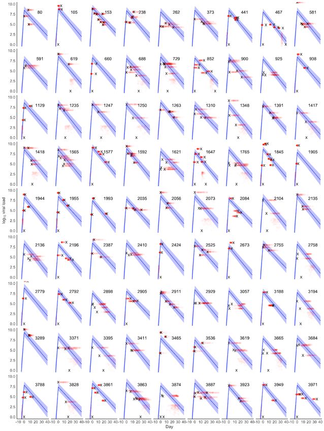
deletion in the spike protein, not of the full complement of B.1.1.7 differences, and confirmatory
full genome sequencing does not seem to have been done. The samples are collected from a
similar time span and region as those in the Golubchik study (below) in which 1299 of 1387
(93.6%) of the samples did not have the N501Y change, so it seems possible that the Kidd et al.
data categorization may not cleanly separate B.1.1.7 from non-B.1.1.7 cases.

The preprint from Golubchik et al. (51) also points in the direction of a higher B.1.1.7 viral load,
but is based on counting the number of mapped sequencing reads. While the authors show a
correlation between number of mapped reads and Ct values, a given number of aligned reads
(e.g., 104 in their Fig. 1) often ranges over about 10 Ct values (i.e., ~3 orders of magnitude)
which cannot be considered a particularly precise quantification for assessing a viral load
difference of ~1, especially with only 88 samples and the likelihood (as the authors clearly state)
of unknown variation in time-of-infection sampling, which our manuscript shows can produce
misleading results.

The preprint from Kissler et al. (52) presents data from seven cases. The difference in the means
is estimated at ~0.3 log10, but three of the seven B.1.1.7 samples show a viral load that is 1 or 2
log10 above the non-B.1.1.7 mean. The 90% credible intervals for the mean viral load are fully
overlapping: (15.8, 22.0) for B.1.1.7 and (19.0, 21.4) for non-B.1.1.7 viral load, from which
nothing can be reliably concluded (and the authors do not make any such claim).

                                                                                                   4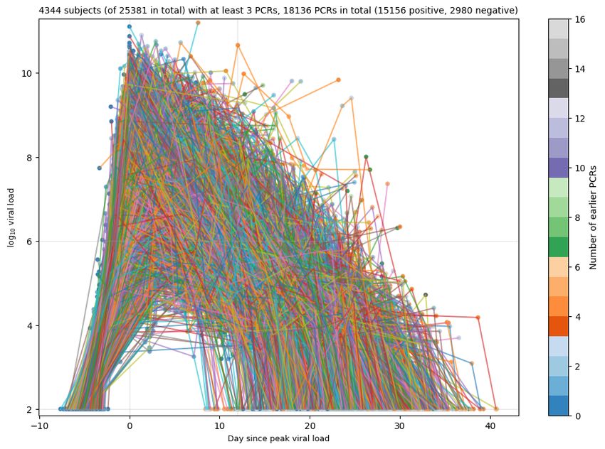
Supplementary Figures

                        5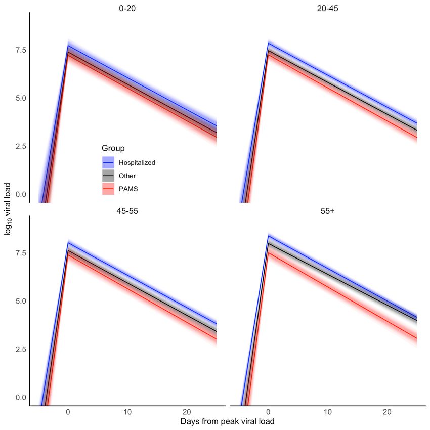
6
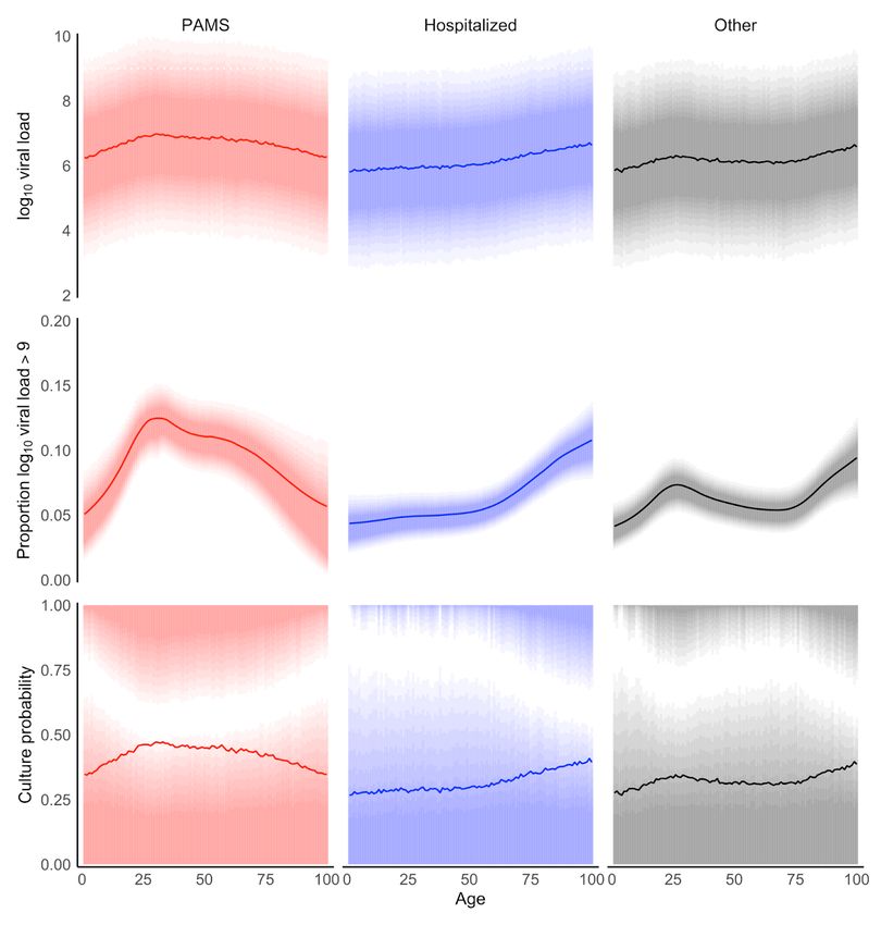
Fig. S1: Estimated and observed mean viral load for subjects younger than 25 years,
stratified by subject group. Observed mean viral loads and 95% confidence intervals are shown
by white points and vertical lines (subject counts are given for each age year and also indicated
by circle size). Model-predicted mean viral loads and credible intervals are shown by the
roughly-horizontal line and shaded region in each plot. Solid black points indicate mean viral
load per age in the full sample.

                                                                                               7
Fig. S2: Mean and 90% highest posterior density regions for posterior predictions of first-
positive viral load and derived variables by age and clinical status. All panels show
predictions for non-B.1.1.7 cases. Top row: log10 viral load at the first positive test. The solid
line indicates the mean. We obtained posterior predictions by applying a post-processing step to
the model-estimated age-wise expected viral loads. The post-processing step estimated, for each
age year, parameters of a mixture of two normal distributions, which was constrained to have the
same mean as the model-estimated viral load and to fit the observed bimodal-distribution of viral
load (cf Fig. 2A). Posterior predictions were then generated from these mixture distributions. The

                                                                                                8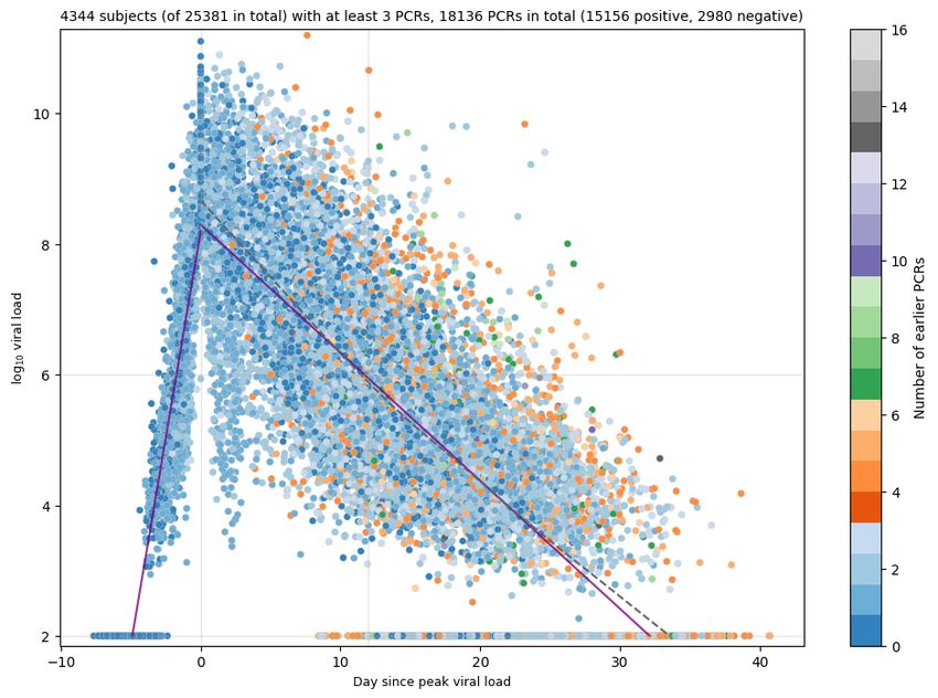
post-processing is further described in the Digital Supplement. Middle row: Estimated
proportion of subjects with high viral loads derived from viral load distributions shown in the top
row. Bottom row: Proportion of positive cultures derived from the top row and the viral load -
culture probability association shown in Fig. 2C. This differs from Fig. 2E which did not use the
post-processing described above.

                                                                                                 9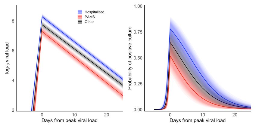
Fig. S3: Characteristics of subjects with first-positive viral load above 9 log10. A) The area of
each rectangle indicates the proportion of participants in the age group. B) Relative risk of being
a high viral load subject at the time of detection, calculated as the proportion of the group among
high viral load subjects divided by the proportion of the same group among all subjects.

                                                                                                 10
Fig. S4: Pre-inoculation viral loads resulting in B.1.1.7 and B.1.177 cell culture isolation
success. Distributions of viral loads from B.1.1.7 and B.1.177 samples for which Caco-2 cell
culture isolation was attempted. The crosses indicate the means and confidence intervals of
culture-positive samples. Viral loads are those obtained from samples prior to cell culture
inoculation. While no statistically significant difference is seen between the means of the viral
load distributions of successful isolations, there are insufficient sample numbers to claim that the
means are the same (Materials and Methods). The many samples with viral loads in excess of 8
that did not result in successful isolation are indicative of sample uncertainty due to the routine
diagnostic laboratory context, including uncontrolled pre-analytical parameters such as
transportation time and temperature.
11Fig. S5: Group-level parameter distributions for the Bayesian model of viral load over
time. The mean values are followed by 90% credible intervals in parentheses. These are results
for the 4344 subjects with RT-PCR results on at least three days.
12Fig. S6: Highest posterior density region (HDR) for peak viral load and culture probability
by clinical status and age. Top row: 90% HDR for estimated peak viral load. The solid line in
each plot indicates the mean. Middle row: 90% HDR for proportion of subjects with a peak
log10 viral load higher than nine. Bottom row: 90% HDR for estimated peak culture probability.
The HDR for the PAMS and Other groups shows a bi-modal distribution of peak culture
probability for some age groups. For PAMS subjects younger than ~40 years, the results suggest
that the majority of participants have a lower culture probability, whereas a minority of subjects
have a high culture probability. For subjects aged ~45 years old, less than 10% have the
estimated mean culture probability.
13Fig. S7: Bayesian viral load time series estimation for subjects with at least three RT-PCR
results. The plot shows the placement in time of 18,136 RT-PCR viral load values from 4344
subjects with at least three RT-PCR results. Points with central black dots indicate the first test of
a subject. Because RT-PCR tests have a limit of detection of around 100 RNA copies (when
sample dilution is accounted for) and false negatives are more likely when the true viral load is
low, we imputed log10 viral load values of negative tests (shown in red, with observed positive-
test viral loads in blue). The permissible range of imputed log10 values for negative tests is -Inf to
+3. Note that choosing a lower upper limit for trailing negative tests would lead to slightly
steeper decrease in viral load. Negative imputed values are allowed to capture situations in which
a leading negative test is followed several days later by low, positive viral load(s). In this
scenario the infection occurred between the leading negative test and the first positive test. The
inset in the bottom right corner shows that fitting a line through the first-positive tests means that
estimated log10 viral loads at the time of the leading negative test should be allowed to be
14negative. However, negative values for imputed log10 viral loads should not be interpreted as
suggesting the presence of a fractional virus particle. Instead, by allowing imputation of negative
log10 viral loads, we calculate a more accurate estimation of increasing viral load at the
beginning of the infection, based on these negative tests that may in fact conceal viral
concentrations below the limit of detection.
1516
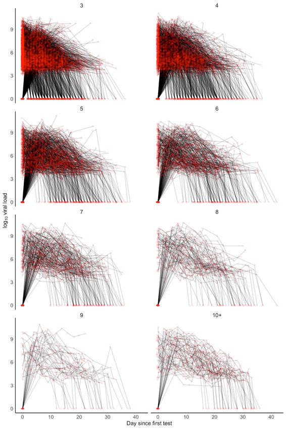
Fig. S8: Raw data of participants with time course data. The red dots show viral load data
points, with results from individuals connected by lines. Panels show data from participants with
different numbers of test results.

                                                                                               17
Fig. S9: Viral load and culture probability time courses according to clinical status. PAMS
and Other subjects have lower viral loads than Hospitalized and thus also infectivity throughout
the infection. This suggests that the higher observed first-positive viral load for PAMS subjects
(Figs. 2A, 2C) is due to those samples being collected at earlier time points in infections.
1819
Fig. S10: Associations between age and subject-level model parameters. A) Slope of viral
load increase. B) Peak viral load. C) Slope of viral load decline. The left column shows
conditional effects, that is the associations with age after adjusting for clinical status, gender, and
random effects of test centers. Gray shading shows 90% credible intervals. The histograms on
the right show posterior distributions of subject-level parameter estimates. The gray histogram at
the bottom of panel C shows the age distribution of the sample.

                                                                                                    20
Fig. S11: Bayesian model parameters according to number of RT-PCR test results. A) Viral
loads from subjects with at least three RT-PCR results were modeled in a single estimation.
Resulting model parameters for subsets of subjects with exactly three, exactly four, etc., results
from this overall estimation are shown. B) Model parameters for seven separate estimations,
involving progressively smaller subsets of subjects with increasingly many RT-PCR results each,
from subjects with at least three results (n=4344) to those with at least nine (n=100). Table S5
provides additional detail regarding cardinality and model parameters, together with a
comparison of parameter values from the alternate simulated annealing approach.
21A
22B
Fig. S12: Simulated annealing viral load time series estimation for subjects with at least
three RT-PCR results. The plots show an example placement in time of 18,136 RT-PCR viral
load values from 4344 subjects with at least three RT-PCR results. The RT-PCR time series for
each subject may include a single negative result before the positive values or a single negative
result after the positives. The 2980 negative outcomes have their viral loads set to 2.0, in
accordance with our SARS-CoV-2 RT-PCR limit of detection calculation and a sample dilution
factor of ~20 (19). A) Each RT-PCR result is shown as a colored dot, where color indicates the
number of earlier RT-PCR results in the time series for the subject in question. The x-axis
intercept of the left-hand side increase line (slope 1.27) gives an estimated time from infection to
peak viral load of 4.89 days. The right-hand side log10 viral load decline line has slope -0.20 per
day and the height of the day zero intercept of the decline line is at viral load 8.30. The slopes of
both lines and the height of their intersection were optimized using a simulated annealing
algorithm that also simultaneously assessed small random adjustments of the time series for each
person forward or backwards in time to better locate it with respect to the day of maximum viral
load (Supplementary Text). Linear regression lines (purple) are separately fitted through the
results that occur before and after the day of peak viral load (x=0). A LOWESS fit (gray dotted
line) is plotted through the points after the peak viral load. The plot shows just one example run.
Statistics for the optimization parameters for subjects with three to nine RT-PCR results over 100
runs are given in Table S5. B) Shows the same data as A, except lines join the successive viral
23load results for each person. This makes it possible to see the overall pattern of viral load rise
and fall based on per-subject trajectories. Dot color is the same as in A. Line colors are
arbitrarily chosen to connect all RT-PCR results for each subject.
24Fig. S13: Estimated viral load courses according to age and clinical status. The figure shows
that, in all age groups and throughout the infection course, Hospitalized patients have the highest
estimated viral load, followed by the Other and then PAMS groups.
25Fig. S14: Viral load time course stratified by primary test center category. The primary test
center category is defined as the one with the longest duration between consecutive tests from
that type. If there are types with equal duration, subjects are assigned to the most severe type in
the order Hospitalized, Other, PAMS. If assignment to a unique category is not possible, a
subject is assigned to a catch-all category (labeled X). Hospitalized patients (e.g., WD, IDW,
ICU) had the highest peak loads, followed by subjects from the Other category (ED, OD, CP).
Patients with COVID-19 test centers (C19) as their primary test center had the lowest viral loads.
The white dotted line shows the mean viral load. Test center abbreviations are described in Table
S1.
26Fig. S15: Patient-reported onset of symptoms compared to estimated day of peak viral
load. The top left histogram is the posterior distribution of the median number of days from peak
viral load to the patient-reported day of symptom onset for the 171 people in the Charité –
Universitätsmedizin cohort with an RT-PCR test time series. The larger histogram shows 4000
overlapping histograms for subject-level estimates, where each histogram shows the distribution
of estimated onset days over the 171 people.
2728
Fig. S16: Posterior predictive check for the estimated time course model with a mixture
model for infection course placement in time. Eighty one arbitrarily-selected posterior
predictions from the 4344 subjects with RT-PCR results on at least three days are shown, to give
an impression of the results of the Bayesian positioning of viral load series in time. Blue lines are
expected viral load time courses, i.e., the average over all time courses, estimated for each
subject. The shaded blue region indicates the 90% credible interval of the expected time course.
The x markers indicate observed measurements, with day zero being the day of the first
measurement. Red points are observed measurements after alignment in time and imputation of
viral loads for negative tests. Numbers are randomly-assigned subject IDs.

                                                                                                  29
Fig. S17: Posterior predictive check for 49 subjects with the highest R-hat values. See Fig.
S16 for an explanation of the graphs. Parameters with R-hat values larger than 1.1 (in
parentheses) are shown in each panel. Large R-hat values are due to time courses that could
either be located at the beginning of the infection, or after viral load decline has begun. Possible
solutions for the placement of the time series for these subjects include a mixture-model
approach for the time series day shift, or a prior that favours negative shifts over positive day
shifts, assuming that infections are more likely to be detected at their beginning. Numbers are
randomly-assigned subject IDs.
30Supplementary tables
Test context Center Center type N N tests N subjects Mean log10 N % Positivity
abbr. positive tested load hosp. hosp. rate
PAMS C19 COVID-19 test center 6159 163,489 71,128 6.9 49 1 3.8
Hospitalized WD Ward 4140 226,691 107,452 6.0 4140 100 1.8
H Hospital 1996 71,745 39,462 6.3 1996 100 2.8
ICU Intensive care unit 630 8,518 5196 6.3 630 100 7.4
IDW Infectious diseases ward 69 186 154 6.1 69 100 37.1
Other ED Emergency department 8224 187,624 131,091 6.5 2457 30 4.4
OD Outpatient department 744 63,296 46,143 5.7 51 7 1.2
AIR Airport 487 41,907 36,799 6.0 3 1 1.2
? Unclassified 634 36,052 22,256 5.9 40 6 1.8
RES Age residence 1121 24,500 9225 6.0 61 5 4.6
PRI Prison 206 13,976 5565 5.7 0 0 1.5
LW Labor ward 99 12,423 10,001 5.5 18 18 0.8
CP Company physician 202 12,406 6747 5.8 4 2 1.6
L Other laboratory (not 455 9964 6691 6.0 1 0 4.6
Labor Berlin)
SM Sports Medicine 116 5921 1301 5.2 0 0 2.0
PHD Public health department 70 813 657 5.5 0 0 8.6
FM Forensic medicine 29 112 80 7.2 0 0 25.9
Table S1: Test center categories and test counts for 25,381 positive subjects. First-positive
RT-PCR tests are broken down according to test center type and category. A context of ‘Other’
is assigned to all centers that are not COVID-19 community centers (C19) or that indicate
subjects who were hospitalized. For example, emergency departments fall into the Other
category because subjects presenting there are not categorized as formally hospitalized at that
point. The number of tests in the denominator of the final column includes all initial negative
tests on subjects, in order to accurately reflect the detection rate according to center type. For
example, if a subject tested negative at the airport, then negative at a sports medicine facility, and
then positive at a COVID-19 test center, all three tests are counted. Note that the table is
primarily focussed on test counts, not subjects. To obtain the subject counts for the PAMS and
Other categories discussed in the main text, sum the “N positive” column for the context and
subtract the sum of the “N hosp.” column to exclude those who were ever hospitalized. Thus the
PAMS category has 6159 - 49 = 6110 subjects, and the Other category has 12,387 - 2635 = 9752
subjects. The total for the Hospitalized category is the sum of the “N positive” column for that
category (6835) plus the hospitalized counts from the PAMS (49) and Other (2635) contexts, so
9519 in total.
31N log10 viral load
Window Model B.1.1.7 non-B.1.1.7 B.1.1.7 non-B.1.1.7 Effect B.1.1.7
Inf unadjusted 1533 23,848 7.3 (7.2, 7.4) 6.3 (6.3, 6.3) 0.99 (0.92, 1.05)
Inf RE, unadjusted 1533 23,848 6.8 (6.7, 6.9) 5.9 (5.8, 5.9) 0.93 (0.86, 0.99)
Inf RE, adjusted 1533 23,848 6.8 (6.7, 6.9) 5.9 (5.8, 5.9) 0.93 (0.86, 0.99)
5 unadjusted 1533 1582 7.3 (7.2, 7.4) 6.3 (6.2, 6.3) 1.04 (0.94, 1.14)
5 RE, unadjusted 1533 1582 7.1 (7.0, 7.2) 6.0 (5.9, 6.2) 1.02 (0.92, 1.11)
5 RE, adjusted 1533 1582 7.2 (7.0, 7.3) 6.1 (6.0, 6.3) 1.04 (0.94, 1.14)
1 unadjusted 1533 977 7.3 (7.3, 7.4) 6.4 (6.2, 6.5) 0.97 (0.85, 1.09)
1 RE, unadjusted 1533 977 7.1 (7.0, 7.2) 6.1 (6.0, 6.2) 1.00 (0.88, 1.11)
1 RE, adjusted 1533 977 7.2 (7.0, 7.3) 6.2 (6.0, 6.3) 1.03 (0.92, 1.14)
1 RE, adjusted, paired 1453 977 7.2 (7.1, 7.4) 6.2 (6.0, 6.4) 1.04 (0.92, 1.15)
Table S2: First-positive viral load comparison between B.1.1.7 and non-B.1.1.7
subjects. Each row shows the estimated effect of B.1.1.7 in an alternative analysis. Window:
Number of days within which non-B.1.1.7 cases must occur in a test center with B.1.1.7 cases to
be included in the analysis: Inf. (all non-B.1.1.7 included), or 5 or 1 for inclusion of non-B.1.1.7
cases detected +/-5 days or +/- 1 day of B.1.1.7 cases. Model: RE test center random effects,
adjusted for age, PCR type, clinical status (PAMS, Hospitalized, Other), and gender; paired: only
test centers that report both B.1.1.7 and non-B.1.1.7 centers are included. Effects are given with
90% credible intervals. N: subject count for B.1.1.7 and non-B.1.1.7 cases. Load: Estimated viral
load (after adjustment, if any). Effect: Viral load difference between B.1.1.7 and non-B.1.1.7
cases.
32Grouping variable Estimate N Increasing slope Days to peak viral load Peak viral load Decreasing slope
Female 2051 1.97 (1.83, 2.13) 4.30 (3.99, 4.62) 8.12 (7.93, 8.30) -0.171 (-0.176, -0.167)
Gender Male 2287 1.97 (1.82, 2.13) 4.32 (3.98, 4.67) 8.16 (7.97, 8.34) -0.165 (-0.170, -0.161)
Female - Male 0.00 (-0.17, 0.17) -0.02 (-0.39, 0.34) -0.03 (-0.12, 0.06) -0.006 (-0.011, 0.000)
Yes 3494 1.92 (1.80, 2.05) 4.46 (4.17, 4.76) 8.27 (8.08, 8.45) -0.169 (-0.172, -0.165)
Hospitalized No 850 2.14 (1.90, 2.42) 3.70 (3.27, 4.16) 7.60 (7.39, 7.79) -0.166 (-0.173, -0.159)
No - Yes 0.22 (-0.02, 0.47) -0.75 (-1.20, -0.30) -0.68 (-0.83, -0.52) 0.003 (-0.005, 0.010)
Yes 262 2.24 (1.88, 2.65) 3.41 (2.84, 4.04) 7.28 (6.95, 7.59) -0.173 (-0.186, -0.159)
PAMS No 4082 1.95 (1.83, 2.08) 4.37 (4.10, 4.66) 8.20 (8.01, 8.37) -0.168 (-0.171, -0.164)
No - Yes -0.29 (-0.68, 0.06) 0.96 (0.33, 1.53) 0.92 (0.62, 1.21) 0.005 (-0.009, 0.018)
Table S3: Viral load time series estimation parameters according to gender and clinical
status. Parameter values and their differences are shown for subject groupings according to
gender, whether the subject was ever hospitalized, and clinical status at time of first-positive RT-
PCR test. The four columns on the right show means and differences in mean for model
parameters, with 90% credible intervals given in parentheses. The slope refers to the gradient of
the log10 viral load increase or decrease. N: number of subjects in the grouping. The Female and
Male subject counts sum to 4338 (not 4344) due to missing gender information for six subjects.
33Age Peak culture Peak viral load Peak culture probability Peak culture probability
Peak viral load
group probability difference to 45-55 difference to 45-55 ratio to 45-55
0-5 7.37 (7.01, 7.77) 0.54 (0.39, 0.71) -0.52 (-0.84, -0.17) -0.15 (-0.26, -0.04) 0.78 (0.61, 0.94)
5-10 7.54 (7.18, 7.91) 0.58 (0.43, 0.75) -0.35 (-0.69, 0.02) -0.11 (-0.22, 0.00) 0.84 (0.69, 1.00)
10-15 7.37 (6.99, 7.79) 0.55 (0.37, 0.73) -0.52 (-0.90, -0.13) -0.14 (-0.27, -0.03) 0.79 (0.60, 0.96)
15-20 7.53 (7.26, 7.81) 0.59 (0.45, 0.73) -0.36 (-0.57, -0.11) -0.10 (-0.17, -0.03) 0.85 (0.74, 0.95)
20-45 7.59 (7.40, 7.78) 0.61 (0.47, 0.73) -0.30 (-0.40, -0.19) -0.08 (-0.12, -0.05) 0.88 (0.82, 0.93)
45-55 7.89 (7.69, 8.09) 0.69 (0.55, 0.81) - - -
55-65 8.10 (7.91, 8.30) 0.74 (0.61, 0.86) 0.21 (0.13, 0.30) 0.05 (0.03, 0.08) 1.08 (1.04, 1.12)
65+ 8.38 (8.19, 8.55) 0.80 (0.67, 0.90) 0.49 (0.38, 0.61) 0.11 (0.08, 0.15) 1.17 (1.10, 1.25)
Table S4: Estimated peak viral load and peak culture probability by age group, with
differences between age groups. Mean peak viral load and culture probability are given, with
90% credible intervals in parentheses. Differences are the younger group minus the older group,
also with 90% credible intervals in parentheses.
34Min. Total Hosp. PCR Positive PCRs PAMS Hospital +ve Method Days to peak Peak viral load Decline slope
PCR subject subjects count (%) +ve PCRs PCRs (%)
days count (%) (%)
3 4344 3494 18,136 15,156 (83.6) 694 (4.6) 10,730 (70.8) SA 4.93 (4.84, 5.02) 8.30 (8.29, 8.31) -0.20 (-0.20, -0.20)
(80.4)
Bayes 4.31 (4.04, 4.60) 8.14 (7.96, 8.32) -0.17 (-0.17, -0.16)
4 2352 1979 12,160 10,202 (83.9) 234 (2.3) 7729 (75.8) SA 4.65 (4.57, 4.73) 8.29 (8.28, 8.30) -0.18 (-0.19, -0.18)
(84.1)
Bayes 4.58 (4.27, 4.89) 8.27 (8.04, 8.51) -0.18 (-0.18, -0.17)
5 1272 1082 7840 6676 (85.2) 78 (1.2) 5206 (78.0) SA 4.59 (4.50, 4.68) 8.32 (8.31, 8.33) -0.18 (-0.18, -0.18)
(85.1)
Bayes 4.52 (4.15, 4.89) 8.21 (7.91, 8.48) -0.18 (-0.18, -0.17)
6 680 592 4880 4203 (86.1) 23 (0.5) 3362 (80.0) SA 4.93 (4.77, 5.09) 8.39 (8.38, 8.40) -0.18 (-0.18, -0.18)
(87.1)
Bayes 4.94 (4.51, 5.38) 8.42 (8.12, 8.69) -0.18 (-0.19, -0.18)
7 371 331 3026 2632 (87.0) 6 (0.2) 2166 (82.3) SA 5.20 (4.98, 5.43) 8.48 (8.47, 8.50) -0.19 (-0.19, -0.19)
(89.2)
Bayes 5.07 (4.58, 5.62) 8.54 (8.16, 8.89) -0.19 (-0.20, -0.19)
8 187 168 1738 1527 (87.9) 4 (0.3) 1290 (84.5) SA 5.36 (4.92, 5.79) 8.58 (8.56, 8.59) -0.19 (-0.19, -0.19)
(89.8)
Bayes 4.80 (4.15, 5.49) 8.60 (8.19, 9.03) -0.20 (-0.21, -0.19)
9 100 91 1042 925 (88.8) 0 (0.0) 812 (87.8) SA 5.93 (5.74, 6.12) 8.50 (8.48, 8.52) -0.19 (-0.19, -0.19)
(91.0)
Bayes 5.27 (4.39, 6.22) 8.49 (7.84, 9.11) -0.19 (-0.21, -0.18)
Table S5: Viral load time series estimation parameters according to minimum number of
RT-PCR results. Parameter values and confidence or credible intervals for two viral load time
series placement estimations: simulated annealing (SA) and a hierarchical Bayesian model
(Bayes). The simulated annealing results for each number of minimum RT-PCR results are
means, computed from 100 independent iterations of the optimization, with a +/- 1.96 standard
deviation range given in parentheses. Columns, left to right: the minimum number of days a
subject must have a RT-PCR result on; the number of subjects with results on at least that many
days; the number (and percentage) of subjects in the Hospitalized category; the total number of
RT-PCR test results in the estimation; the number (and percentage) of positive results; the
number (and percentage) of positive results obtained in a test center detecting PAMS infections;
the number (and percentage) of positive results obtained in a hospital; the estimation method; the
estimated number of days from infection to peak viral load; the estimated peak viral load; and the
estimated slope of the viral load decline line (linear in change in log10 viral load, i.e., exponential
decline).
35You can also read