Leveraging Convolutional Pose Machines for Fast and Accurate Head Pose Estimation - Idiap Publications
←
→
Page content transcription
If your browser does not render page correctly, please read the page content below
Leveraging Convolutional Pose Machines
for Fast and Accurate Head Pose Estimation
Yuanzhouhan Cao1 , Olivier Canévet 1 and Jean-Marc Odobez1,2
Abstract— We propose a head pose estimation framework
that leverages on a recent keypoint detection model. More
specifically, we apply the convolutional pose machines (CPMs)
to input images, extract different types of facial keypoint
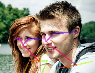
features capturing appearance information and keypoint re- Fig. 1: Example of body landmark detection with CPM [3].
lationships, and train multilayer perceptrons (MLPs) and con-
volutional neural networks (CNNs) for head pose estimation. We are interested in using the predictions of the nose, eyes,
The benefit of leveraging on the CPMs (which we apply anyway and ears to estimate the head pose (yaw, pitch, and roll)
for other purposes like tracking) is that we can design highly
efficient models for practical usage. We evaluate our approach In this paper, we propose to use the landmark detections as
on the Annotated Facial Landmarks in the Wild (AFLW) well as the features of the CPMs to predict the head pose. Our
dataset and achieve competitive results with the state-of-the- work is motivated by the fact that the detections of the CPMs
art.
(namely the nose, eyes, and ears) are extremely reliable (see
Fig. 1), and that the CPMs is often applied anyway for scene
I. I NTRODUCTION
perception, e.g. for tracking people. In this context, the head
Head pose estimation has been a difficult research topic pose can be obtained as a by-product on top of the CPMs.
in computer vision for decades. It can be exploited for Our head pose estimation system is illustrated in Fig. 2.
head gesture recognition [4], and more importantly, as a For a given input color image, we first apply the CPMs to
proxy for gaze [5], it is an important non-verbal cue that extract features including keypoints, confidence maps, and
can inform about the attention of people by itself [1]. As feature maps. Then we train a predictor to output the head
such, it can be used in many human analysis tasks and in pose from them. In this contex, our contributions are:
particular for human-robot interaction (HRI) [7], [18], [8], • We investigate several strategies to leverage the output
social event analysis [12], driver assistance system [2], and of the CPMs (landmarks, confidence maps, features);
gaze estimation [6]. The purpose of head pose estimation is • We investigate several predictors (multilayer percep-
to predict the head pose expressed as three rotation angles trons, convolutional neural networks);
(roll, pitch, yaw). Conventional methods estimate the head • We investigate several strategies for head pose estima-
pose either by fitting facial points to a 3D model [21], tion (pose angle regression, pose likelihood regression).
[13], [19], matching facial point clouds with pose candidates • We achieve competitive head pose predictors making an
through a triangular surface patch descriptor [14], or using error of less than 10◦ for roll, pitch, and yaw.
bayesian methods, especially for tracking tasks [17]. Our system can be viewed as a simple strategy on top of the
Recently, head pose estimation considerably benefit- CPMs to estimate the head pose of detected persons1 .
ted from the success of convolutional neural networks
(CNNs) [9]. Ranjan et al. [16] propose a unified deep II. C ONVOLUTIONAL POSE MACHINES
learning framework for head pose estimation, face detection, The first part of our head pose estimation approach is
landmark localization and gender recognition. Patacchiola et to extract features capturing appearance information and
al. [15] propose a deep learning model to estimate the head facial keypoint relationships. We apply the convolutional
pose of in-the-wild face images. Other works also include pose machines (CPMs) [3] to extract the features.
depth data in CNNs, like Borghi et al. [2] which generate The CPM is a real-time multi-person keypoint detection
face from depth data to predict the head pose of drivers. model (see Fig. 1 for an illustration). In the rest of the paper,
Apart from head pose, body pose and body landmark we equally use keypoint and landmark to name the body
detection have also considerably improved, e.g. with the part predicted by the CPMs. We illustrate the architecture of
introduction of the convolutional pose machines (CPMs) [3]. the CPMs in Fig. 2. It takes as input a color image of size
The CPMs aim at localizing the body landmarks (eyes, ears, h × w and simultaneously output body part confidence maps
nose, shoulders, etc.) and the body limbs (arms, legs, etc.) and affinity fields that encode part-to-part association. The
and leverage the context by iteratively refining its predictions. color image is first fed into a VGG-19 network, generating
Fig. 1 depicts CPM results on some face images. a set of feature maps F that is input to the following stages.
1 Idiap Research Institute, Switzerland. yuanzhouhan.cao@idiap.ch, 1 The code to train the model and to run a real time demo on a
olivier.canevet@idiap.ch, odobez@idiap.ch webcam is available at https://gitlab.idiap.ch/software/
2 Ecole Polytechnique Fédérale de Lausanne (EPFL), Switzerland. openheadpose.
Convolutional Pose Machine                       CPM Output

                                                        S
            color image                      Branch 1                                     keypoints

                                                        L                                                    MLPs/
                                       F                              Stage t       confidence maps                     head pose
              h× w          VGG 19           Branch 2                  (t ≥ 2)
                                                                                                             CNNs

                                                                                       feature maps

Fig. 2: Architecture of our head pose estimation system. It takes as input the color images and outputs CPM features. The
CPM features are fed into MLPs or CNNs for head pose estimation.
                                                                                      (a)                  (b)                 (c)
Each stage contains two branches that have same network
                                                                                 coordinates          confidence maps      feature maps
structures. The top branch produces a set of confidence maps
S and the bottom branch produces a set of affinity fields L.
After each branch, the feature maps F, the confidence maps                       fc 64, relu          5x5 conv 512,      9x9 conv 512,
                                                                                                           relu               relu
S and the affinity fields L are concatenated to be the input
of the following stage. More stages lead to more refined                                                                             /2

predictions. In this paper, we use the CPMs with 6 stages.                       fc 128, relu                            9x9 conv 128,
                                                                                                                 /2
   What makes the CPM very efficient is that it makes use                                                                     relu
of the context and of powerful VGG features, by refining                                                                             /2
its own predictions all along stages t ≥ 2, which leads to                                            5x5 max pool        9x9 max pool
accurate localization of the body joints.                                                                        /2                  /2
   During training, two L2 loss functions are applied at the                         fc                    fc                  fc
end of each stage, one at each branch respectively. The loss
values of both branches are added up and backpropagated
to update network weights. In our head pose estimation, we                       Head Pose             Head Pose           Head Pose
apply the CPMs trained on the Microsoft COCO dataset [10]
with 18 body keypoints (including nose, eyes, ears, and                   Fig. 3: Structures of our proposed head pose estimation
shoulders) to extract the features. We directly apply this                models. (a) MLPs taking as input keypoint coordinates. (b)
network without finetuning.                                               CNNs taking as input the confidence maps of keypoints. (c)
                                                                          CNNs taking as input feature maps. The number of hidden
                  III. P ROPOSED METHOD                                   nodes in the last fully-connected layer depends on the loss.
   In this section, we elaborate our head pose estimation
approach. Specifically, for an input image, we first obtain the           to be the face center. The width w of the face region is
keypoints, the confidence maps, and the feature maps through              defined as the horizotal distance between two eyes, and the
the CPMs. Then we train multilayer perceptrons (MLPs) or                  height h is defined as the larger vertical distance between the
convolutional neural networks (CNNs) to predict the head                  nose and the two eyes. The normalized coordinate vectors
pose expressed as angles of pitch, roll and yaw.                          of all the keypoints are concatenated to be the input of our
A. Keypoint-based head pose estimation                                    head pose estimation model. Since some keypoints may not
   The outputs of the CPM are confidence maps and part                    exist in an input image, the concatenated coordinate vector
affinity fields. The position of a body keypoint can be                   contains missing values. We apply the probabilistic principal
obtained by selecting the pixel with the maximum confidence               analysis (PPCA) [20] to fill these missing values.
value that is above a predefined threshold. If all the values                We train multilayer perceptrons (MLPs) for head pose
in a confidence map are smaller than the threshold, then                  estimation. The structure of our MLPs is illustrated in
the corresponding keypoint is considered not to be in the                 Fig. 3(a). It contains 3 fully-connected layers and rectified
input image. The position of a keypoint is represented as a               linear units (ReLUs) are applied after the first two fully-
two dimensional coordinate vector (x, y). Since our task is               connected layers. The MLPs take as input the normalized
to estimate the head pose, we only consider 8 keypoints in                coordinates of keypoints and output the head pose.
the upper body: nose, neck, eyes, ears and shoulders. The                 B. CPM-feature based head pose estimation
obtained coordinate is normalized as:

                                x − xc y − yc
                                                                            In order to achieve more accurate head pose estimation,
                 (xn , yn ) =         ,         ,         (1)             for an input image, we extract deeper features from different
                                  w      h
                                                                          layers of the CPMs and train convolutional neural networks
where (xc , yc ) is the center of the face region and (w, h) is           (CNNs). Specifically, we extract the confidence maps and
the size of the face region. In practice, we use the center of            the feature maps. The structure of CNNs trained on the
nose and eyes:                                                            confidence maps are illustrated in Fig. 3(b). It contains one

                  xnose + xleye + xreye ynose + yleye + yreye             convolution layer, one ReLU, one max pooling layer and one
   (xc , yc ) =                        ,                        (2)
                           3                     3                        fully-connected layer.
As for the feature maps, we extract the output of two ground-truth angle d in radians, we generate two gaussian
different layers from the CPMs: the output of the VGG- distributions with a variance σ , and the mean values are
19 network (F in Fig. 2), and the output of the second d and d − 2π (shown in red and blue) respectively. For
last convolution layer of the Branch 2 in the last stage. each bin, we assign the maximum value of the two gaussian
The dimension of the two sets of feature maps is 128. distributions to be the likelihood of the corresponding angle
The structure of the CNNs trained on these feature maps range.
is illustrated in Fig. 3(c). It contains two convolution layers When our models predict angle likelihoods, b in Eq. 3
followed by two ReLUs, one max pooling layer and one is the number of bins. The last fully-connected layers
fully-connected layer. in Fig. 3 have 3b hidden nodes. y = (lr > , lp > , ly > ) and
Our CNNs for head pose estimation take as input the face y∗ = (l∗r > , l∗p > , l∗y > ) in Eq. 3 are predicted and ground-truth
regions in the CPM features. We crop the face regions based likelihoods respectively.
on the positions of nose and eyes as illustrated in Fig. 4.
We first get the vertical distance d between the nose and the π
2
center of the eyes. Then we crop a square of size 5d × 5d
around the nose, with 3d above the nose, 2d below the nose,
2.5d left and right to the nose. The positions of nose and eyes
are predicted by the CPMs. In our experiments, we also crop - π d π
the face regions according to the ground-truth face rectangles
ground truth angle ground-truth likelihoods
of the dataset. The height and the width of the cropped face
regions are rescaled to 128.
Fig. 5: Conversion of ground-truth angles to likelihoods.
The values of likelihoods are generated from two gaussion
distributions with mean values of d and d − 2π (shown in
red and blue) respectively, where d is the ground-truth angle
in radians.
d
IV. E XPERIMENTS
We now present the results of our method of head pose
estimation. We show that our method is able to leverage the
CPMs output and yields competitive results with the state-
Fig. 4: Illustration of cropping. We crop the face regions of-the-art Hyperface model.
in the confidence maps and the feature maps based on the
positions of nose and eyes. A. Dataset
We evaluate our head pose estimation on the Annotated
C. Loss function Facial Landmarks in the Wild (AFLW) dataset [11]. The
AFLW is a large-scale, multi-view, real-world face dataset
Our head pose estimation models are trained by minimiz-
gathered from Flickr, exhibiting a large variety in face
ing the mean squared error (MSE) between the predictions
appearance (e.g. pose, expression, ethnicity, age, gender) as
and the ground-truth values, defined as:
well as general imaging and environmental conditions. It
11 3 b contains about 25k faces annotated with facial landmarks,
L(y, y∗ ) = ∑ ∑ (y p (i) − y∗p (i))2 . (3) face rectangles, head pose, etc. In our experiments, the input
3 b p=1 i=1 to the convolutional pose machine (CPMs) network is the
We consider two types of model predictions: angles and AFLW faces with the largest possible contexts.
angle likelihoods. When our models directly predict the head
pose expressed as roll, pitch and yaw angles, the last fully- B. Evaluation protocol
connected layers in Fig. 3 have 3 hidden nodes. The value We divide the AFLW into train, validation, and test sets:
of b is 1 in Eq. 3 and y = (ar , a p , ay ) and y∗ = (a∗r , a∗p , a∗y ) for all the faces in the AFLW dataset, there are 17,081 faces
are model prediction and ground-truth respectively. with nose and two eyes annotated, and 19,887 faces with
The angles of roll, pitch and yaw are periodic. Consider nose and two eyes detected by the CPMs. We select an
a ground-truth value of 0◦ , the predictions of 1◦ and 359◦ intersection of 15,230 faces, and randomly split these images
should have the same loss values. Directly predicting the into a training set of 9,138 images, and a validation set and
pose angles does not consider this discontinuity. In addition, a test set of 3,046 images each.
the predictions lack confidence. In order to solve these To allow a fair comparison with the Hyperface method
drawbacks, we convert the ground-truths from angles to angle which also uses the AFLW dataset, we contact the authors
likelihoods as illustrated in Fig 5. Specifically, we first evenly to get their own train and test sets. This other “split” of the
discretize the range of [−π, π] into several bins. Then for a AFLW is only used in Table V for comparison.We apply the following measures to evaluate the head pose TABLE I: Head pose estimation results based on facial
estimation: keypoint positions. The first two rows are MLPs trained with
3 keypoints and 5 keypoints estimated by the CPMs. The
• mean absolute error (MAE): N ∑n |yn − y∗n |, where y∗n is
1
last row are the results of MLPs trained with 5 ground-truth
the ground truth value (roll, pitch or yaw) of image n, yn
keypoints.
is the estimated value by our method, and N is the total
number of images in the test set. This MAE represents Accuracy (%) Error
the error that our method does in estimating the three δ < 5◦ δ < 10◦ δ < 15◦ MAE
angles. r: 68.8 r: 87.9 r: 93.5 r: 5.04
3 keypoints
• accuracy with threshold τ: percentage of yn s.t. p: 33.6 p: 60.1 p: 78.7 p: 9.53
from CPM
|yn − y∗n | = δ < τ, where yn is the estimated value and y: 35.5 y: 62.5 y: 77.5 y: 10.65
y∗n the ground truth. The “accuracy below a threshold” is 5 keypoints r: 71.9 r: 89.2 r: 94.1 r: 4.72
p: 43.4 p: 72.6 p: 89.0 p: 7.52
an interesting cue because an error of 10◦ (for example) from CPM
y: 44.9 y: 70.9 y: 83.6 y: 9.19
in the estimation is actually very small to the human
eye. This score considers correct an estimation which 5 AFLW annotations r: 85.8 r: 97.9 r: 99.4 r: 2.77
(sanity check)
p: 49.9 p: 78.6 p: 92.1 p: 6.45
is below threshold τ from the correct value. y: 55.6 y: 85.5 y: 96.5 y: 5.46
C. Keypoint-based head pose estimation results
In this section, we evaluate our MLPs trained on the regions in the confidence maps are cropped using the ground-
coordinate vectors of keypoints (see Sec. III-A). As explained truth face rectangles without contexts. In order to crop the
in Sec. IV-A, we only kept the images from AFLW for which neck and shoulders in the confidence maps with 8 keypoints,
the CPMs could detect the nose and both eyes. we crop the ground-truth face rectangles with some contexts.
We train two MLPs, one by using 3 keypoint coordinates Specifically, 25% of the hight above, 75% of the hight below,
(nose and two eyes), and another one by using 5 keypoints 50% of the width left and right. From Table II we can see
(two ears in addition). These keypoints are the coordinates that experiment with more keypoint confidence maps leads
of the detected keypoints by the CPMs (see Fig. 1 as an to better performance (row “5 confidence maps from stage 6”
illustration). better than row “3 confidence maps from stage 6”). However,
Table I shows the results of the two networks. The MLPs using 8 keypoints does not further improve the performance,
trained on 3 keypoints achieve an error of 10.65◦ on average this is caused by the inconsistency of shoulders and head, as
for the yaw, and an accuracy of 62.5% with a 10◦ threshold. a front looking face may have multiple shoulder positions.
The MLPs trained on 5 keypoints achieve an error of The confidence maps in the aforementioned experiments
9.19◦ for the yaw, and an accuracy of 70.9% with a 10◦ are extracted from the last stage (stage 6) of the CPM. We
threshold. We can see that using more keypoints yields better have also investigated the use of features in the earlier stages
performance. of the CPM, namely stage 1 and stage 3 (rows “5 confidence
As a sanity check, we also train MLPs with the ground- maps from stage 1” and “5 confidence maps from stage 3”),
truth annotations of the AFLW dataset. This corresponds which are less refined that in stage 6. We observe that that our
to the ideal case where we train with perfect locations (as CNN models trained on the confidence maps of stage 6 have
opposed to keypoints detected by CPMs as in the previous the best performance. We can conclude that the late feature
2 cases). We see in Table I that with more accurate locations are better for head pose estimation, which was expected as
of face landmarks, we can achieve more satisfactory pose the late features are more refined, and better localize the
estimations: 5.46◦ average error for the yaw, and 96.5% body landmarks.
accuracy with a 10◦ threshold.
We have also investigated the cropping of the face regions
D. CPM-feature based head pose estimation results from confidence maps. So far, the face regions are cropped
using the ground-truth face rectangles in the AFLW dataset.
In this section we present our head pose estimation re- However, in practice, the ground-truth rectangles are not
sults based on the confidence maps and the feature maps available. We crop the face areas using the CPM estimated
respectively. We also show the results of the angle likelihood facial keypoints as illustrated in Sec. III-B. We also crop
regression. the face areas with some additional context. Specifically,
Confidence map-based. Each confidence map represents the we crop a square of size 10d × 10d centred at the nose,
probability of existence of a body landmark (or keypoint) at where d is the vertical distance between the nose and the
all the positions of an input image. We train convolutional center of eyes in Fig. 4. From the table, rows “5 confidence
neural networks with different number of keypoints and show maps + estimated cropping” and “[...] context”, we can see
the results in the first 4 rows of Table II. Specifically, the 3 that the results of cropping using ground-truth face rectangles
keypoints are nose and eyes, the 5 keypoints are the 3 key- (i.e. AFLW annotations) outperform the results of cropping
points plus ears, and the 8 keypoints are the 5 keypoints plus using estimated facial keypoints. The performance can be
neck and shoulders. All the confidence maps are extracted further improved with more accurate face localization. Some
from the last stage of the CPM network (stage 6). The face cropping examples are shown in Fig. 6.TABLE II: Head pose estimation based on confidence maps
Est
with the variation of number of keypoints. By default, the
confidence maps are extracted from the last stage. The “con-
text” indicates that the confidence maps are cropped with
Est
Context contexts, and the “estimated” indicates that the confidence
maps are cropped based on the CPM estimated keypoints.
GT Accuracy (%) Error
δ < 5◦ δ < 10◦ δ < 15◦ MAE
3 confidence maps r: 80.2 r: 95.8 r: 98.2 r: 3.38
from stage 6
p: 44.7 p: 76.6 p: 91.8 p: 6.91
GT y: 44.1 y: 74.7 y: 89.2 y: 7.40
Context
8 confidence maps r: 79.1 r: 94.7 r: 97.8 r: 3.59
from stage 6
p: 45.0 p: 77.8 p: 92.4 p: 6.69
y: 45.2 y: 74.2 y: 89.2 y: 7.45
Fig. 6: Cropping examples. The first two rows are the exam- 8 confidence maps r: 73.2 r: 92.7 r: 97.2 r: 4.06
ples of cropping using estimated facial keypoints without from stage 6 p: 43.0 p: 75.0 p: 90.4 p: 7.13
and with context respectively. The second two rows are + context y: 45.0 y: 73.6 y: 87.4 y: 7.64
the examples of cropping using ground-truth face rectangles 5 confidence maps r: 80.3 r: 95.7 r: 98.2 r: 3.37
from stage 6
p: 46.5 p:79.0 p: 92.9 p: 6.55
without and with context respectively. y: 46.9 y:76.2 y: 90.1 y: 7.04
5 confidence maps r: 76.0 r: 93.1 r: 97.0 r: 3.91
from stage 1
p: 44.9 p: 76.9 p: 92.0 p: 6.76
y: 42.7 y: 72.4 y: 86.6 y: 8.02
Overall, we can see from Table II that using 5 keypoint
confidence maps yields the best estimation of the head pose. 5 confidence maps r: 73.8 r: 92.3 r: 97.3 r: 4.13
from stage 3
p: 42.4 p: 73.6 p: 89.9 p: 7.25
y: 44.5 y: 73.2 y: 87.5 y: 7.66
Feature map-based. We are now interested in whether the
features of the first part of the CPM (i.e. VGG features) are 5 confidence maps r: 75.5 r: 92.3 r: 96.0 r: 4.09
+ estimated cropping
p: 43.9 p: 74.6 p: 90.5 p: 7.12
sufficient for head pose estimation. To this purpose, we train y: 40.8 y: 68.3 y: 82.7 y: 9.08
a first network taking as input feature maps from the VGG- 5 confidence maps, r: 66.3 r: 87.4 r: 94.3 r: 5.15
19 network (F in Fig. 2), and another network that takes as + estimated cropping p: 42.0 p: 72.5 p: 89.3 p: 7.47
+ context y: 37.3 y: 64.6 y: 79.2 y: 9.96
input the second last convolution layer of Branch 2 in the last
stage. Both of the feature maps have 128 channels. We crop
the face regions using the ground-truth face regions without TABLE III: Head pose estimation using feature maps ex-
context. The results are illustrated in Table III, from which tracted from different layers of the CPM network. The first
we can see that the results using the feature maps of the last row are the results of using the output of the VGG-19
stage significantly outperform the results using the VGG-19 network (F in Fig. 2), the second row are the results of using
feature maps. This makes sense since the features of stage 6 the output of the second last convolution layer of Branch 2
are specifically trained for body parts, especially nose, ears, in the last stage.
and eyes.
Accuracy (%) Error
Angle likelihood regression. In all the aforementioned δ < 5◦ δ < 10◦ δ < 15◦ MAE
experiments, the outputs of the CNNs are pose angles. The r: 43.6 r: 67.2 r: 80.7 r: 9.14
Features F
CNNs are trained by minimizing the mean square errors be- from VGG
p: 31.7 p: 58.3 p: 77.1 p: 9.87
tween ground-truth and estimated angles. In this section, we y: 20.1 y: 35.9 y: 48.2 y: 18.60
train CNNs by minimizing the mean square errors between Last features r: 79.9 r: 95.8 r: 98.3 r: 3.44
from stage 6
p: 49.0 p:81.8 p: 94.4 p: 6.10
ground-truth and estimated angle likelihoods, as illustrated y: 51.4 y: 80.5 y: 92.8 y: 6.41
in Sec. III-C. The inputs of the CNNs are confidence maps
of 5 facial keypoints generated from the last stage of the TABLE IV: Head pose estimation using angle likelihood
CPM, and the face regions are cropped with the ground-truth regression. The ground-truth likelihoods are generated with
face rectangles without context. We discretize the range of different number of discretizing bins and σ in Sec. III-C.
[−π, π] into different number of bins, and use the Gaussian
distributions with different variance σ . We report the errors σ = 0.1 σ = 0.3 σ = 0.5
in Table IV. As we can see from the table that the best r: 5.33 r: 3.86 r: 3.88
performance is achieved when the number of bins is 180 180 bins p: 7.36 p: 7.14 p: 7.09
and σ = 0.3. But the results are roughly the same as by y: 7.47 y: 7.04 y: 7.38
directly regressing the angles. r: 5.75 r: 4.07 r: 4.05
240 bins p: 7.48 p: 7.28 p: 7.28
y: 7.65 y: 7.25 y: 7.52
E. Stage-of-the-art comparison
r: 5.87 r: 4.18 r: 4.19
In this section, we compare our head pose estimation 360 bins p: 7.72 p: 7.32 p: 7.36
y: 7.85 y: 7.34 y: 7.71
method with the Hyperface method [16].TABLE V: Head pose estimation on the Hyperface split the success of the CPM, our system can be seen as a simple
of the AFLW dataset. The first 4 rows are results of our method to get head pose as a by-product of the CPM.
approach and the last row are the results in [16]. Our
models are trained using feature maps. The “GT” and “Est” VI. ACKNOWLEDGEMENT
indicate the face region cropping scheme, and the “angle” This work was supported by the European Union under the EU
and “likelihood” indicate the loss function during training. Horizon 2020 Research and Innovation Action MuMMER (Mul-
tiModal Mall Entertainment Robot), grant agreement no. 688147,
Accuracy (%) Error http://mummer-project.eu/.
δ < 5◦ δ < 10◦ δ < 15◦ MAE
r: 71.4 r: 91.1 r: 96.2 r: 4.58 R EFERENCES
GT, angle p: 50.4 p: 79.6 p: 93.1 p: 6.34 [1] S. Ba and J. Odobez. A study on visual focus of attention recognition
y: 45.6 y: 72.3 y: 86.1 y: 8.21 from head pose in a meeting room. In Proc. Workshop on Machine
r: 73.5 r: 92.1 r: 96.6 r: 4.21 Learning for Multimodal Interaction (MLMI), May 2006.
GT, likelihood p: 48.9 p: 79.1 p: 91.6 p: 6.57 [2] G. Borghi, M. Venturelli, R. Vezzani, and R. Cucchiara. Poseidon:
y: 46.5 y: 73.0 y: 86.4 y: 8.43 Face-from-depth for driver pose estimation. 2017.
[3] Z. Cao, T. Simon, S.-E. Wei, and Y. Sheikh. Realtime multi-person
r: 64.8 r: 85.6 r: 93.6 r: 5.54
Est, angle p: 46.5 p: 76.5 p: 90.0 p: 7.23 2d pose estimation using part affinity fields. In CVPR, 2017.
[4] C. Chen, Y. Yu, and J.-M. Odobez. Head nod detection from a full
y: 39.1 y: 65.1 y: 76.8 y: 11.38
3d model. In Int. Conf. on Computer Vision Workshop,, 2015.
r: 66.6 r: 86.3 r: 93.6 r: 5.37 [5] K. Funes and J.-M. Odobez. Person independent 3d gaze estimation
Est, likelihood p: 42.9 p: 74.0 p: 88.4 p: 7.57 from remote rgb-d cameras. In ICIP, 2013.
y: 40.2 y: 67.5 y: 81.2 y: 10.58 [6] K. A. Funes Mora and J.-M. Odobez. Gaze estimation in the 3d space
using rgb-d sensors: Towards head-pose and user invariance. Int. J.
r: 76.0 r: 95.0 r: 97.0 r: 3.92 Comp. Vis., 2017.
Hyperface p: 51.0 p:81.0 p: 95.0 p: 6.13 [7] M. A. Goodrich and A. C. Schultz. Human-robot interaction: A survey.
y: 46.0 y: 76.0 y: 89.0 y: 7.61 Found. Trends Hum.-Comput. Interact., 1(3), 2007.
[8] M. F. Jung. Affective grounding in human-robot interaction. In IEEE
Int. Conf. Hum.-Robot Interact., 2017.
[9] A. Krizhevsky, I. Sutskever, and G. E. Hinton. Imagenet classification
For a fair comparison with the Hyperface method which with deep convolutional neural networks. In NIPS. 2012.
also uses the AFLW, we contact the authors to get their own [10] T.-Y. Lin, M. Maire, S. Belongie, J. Hays, P. Perona, D. Ramanan,
P. Dollár, and C. L. Zitnick. Microsoft coco: Common objects in
train and test sets of the AFLW. So here, neither the train context. In Proc. Eur. Conf. Comp. Vis., 2014.
set nor the test set is the same as in the previous sections. [11] P. M. R. Martin Koestinger, Paul Wohlhart and H. Bischof. Annotated
Our CNNs are trained on the feature maps that are ex- Facial Landmarks in the Wild: A Large-scale, Real-world Database
for Facial Landmark Localization. In Proc. First IEEE Int. Workshop.
tracted from the second last convolution layer of the Branch Benchmarking Facial Image Anal. Technol., 2011.
2 in the last stage of the CPM. During training, we apply [12] S. Muralidhar, L. S. Nguyen, D. Frauendorfer, J.-M. Odobez,
M. Schmid Mast, and D. Gatica-Perez. Training on the job: Behavioral
the regression on both pose angles and likelihoods. The analysis of job interviews in hospitality. In ACM ICMI, 2016.
face regions in the features maps are cropped using both [13] G. P. Meyer, S. Gupta, I. Frosio, D. Reddy, and J. Kautz. Robust
ground-truth face rectangles as well as the CPM estimated model-based 3d head pose estimation. In Proc. IEEE Int. Conf. Comp.
Vis., 2015.
facial keypoints without contexts. We show the results in [14] C. Papazov, T. K. Marks, and M. Jones. Real-time 3d head pose and
Table V. Note that the accuracies in [16] are reported as facial landmark estimation from depth images using triangular surface
curves in a 2-D coordinate system, with the x axis to be patch features. In Proc. IEEE Conf. Comp. Vis. Patt. Recogn., 2015.
[15] M. Patacchiola and A. Cangelosi. Head pose estimation in the wild
the thresholds and y axis to be the accuracies. We obtain using convolutional neural networks and adaptive gradient methods.
the rough accuracies of δ < 5◦ , δ < 10◦ , δ < 15◦ from these Pattern Recogn., 71, 2017.
[16] R. Ranjan, V. M. Patel, and R. Chellappa. Hyperface: A deep multi-
curves. We can see that our approach, yields competitive task learning framework for face detection, landmark localization, pose
results with the Hyperface. More importantly, our method estimation, and gender recognition. IEEE Trans. Pattern Analysis and
takes much less time to process. As reported in [16], on Machine Intelligence, 2017.
[17] E. Ricci and J. Odobez. Learning large margin likelihood for realtime
a GTX TITAN-X GPU, it takes the Hyperface 3 seconds head pose tracking. In IEEE International Conference on Image
output head pose from an image. We test our method on a Processing, november 2009.
[18] S. Sheikhi and J. Odobez. Combining dynamic head pose and gaze
GTX 1080-TI GPU, and it takes around 0.0001 seconds to mapping with the robot conversational state or attention recognition in
output head pose from a confidence map, and around 0.2 human-robot interactions. Pat. Recog. Letters, 66:81–90, Nov. 2015.
seconds to output head pose from an image (including the [19] M. Storer, M. Urschler, and H. Bischof. 3d-mam: 3d morphable
appearance model for efficient fine head pose estimation from still
CPM processing) images. In Proc. IEEE Int. Conf. Comp. Vis. Workshops, 2009.
[20] M. E. Tipping and C. M. Bishop. Probabilistic principal component
V. C ONCLUSION analysis. J. of the Royal Stat. Society, 61:611–622, 1999.
[21] Y. Yu, K. A. F. Mora, and J. Odobez. Robust and accurate 3d head
We have proposed a head pose estimation approach lever- pose estimation through 3dmm and online head model reconstruction.
aging the convolutional pose machines. Our method takes as In Int. Conf. Auto. Face Gesture Recogn., 2017.
input either facial keypoints, or confidence maps, or feature
maps of the CPMs. We have shown that such method can
obtain competitive performance with the state-of-the-art.
Given the impact of face localization on performance, one
future direction is to learn how the face should be cropped
before applying our pose estimation method. Overall, withYou can also read