Interlinked Convolutional Neural Networks for Face Parsing
←
→
Page content transcription
If your browser does not render page correctly, please read the page content below
Interlinked Convolutional Neural Networks for
                                                            Face Parsing

                                                                  Yisu Zhou, Xiaolin Hu, Bo Zhang

                                                     State Key Laboratory of Intelligent Technology and Systems
                                            Tsinghua National Laboratory for Information Science and Technology (TNList)
                                                          Department of Computer Science and Technology
                                                             Tsinghua University, Beijing 100084, China
arXiv:1806.02479v1 [cs.CV] 7 Jun 2018

                                                Abstract. Face parsing is a basic task in face image analysis. It amounts
                                                to labeling each pixel with appropriate facial parts such as eyes and
                                                nose. In the paper, we present a interlinked convolutional neural network
                                                (iCNN) for solving this problem in an end-to-end fashion. It consists of
                                                multiple convolutional neural networks (CNNs) taking input in differ-
                                                ent scales. A special interlinking layer is designed to allow the CNNs
                                                to exchange information, enabling them to integrate local and contex-
                                                tual information efficiently. The hallmark of iCNN is the extensive use
                                                of downsampling and upsampling in the interlinking layers, while tra-
                                                ditional CNNs usually uses downsampling only. A two-stage pipeline is
                                                proposed for face parsing and both stages use iCNN. The first stage lo-
                                                calizes facial parts in the size-reduced image and the second stage labels
                                                the pixels in the identified facial parts in the original image. On a bench-
                                                mark dataset we have obtained better results than the state-of-the-art
                                                methods.

                                                Keywords: Convolutional neural network, face parsing, deep learning,
                                                scene labeling

                                        1     Introduction

                                        The task of image parsing (or scene labeling) is to label each pixel in an im-
                                        age to different classes, e.g., person, sky, street and so on [1]. This task is very
                                        challenging as it implies jointly solving detection, segmentation and recognition
                                        problems [1]. In recent years, many deep learning methods have been proposed
                                        for solving this problem including recursive neural network [2], multiscale convo-
                                        lutional neural network (CNN) [3] and recurrent CNN [4]. To label a pixel with
                                        an appropriate category, we must take into account the information of its sur-
                                        rounding pixels, because isolated pixels do not exhibit any category information.
                                        To make use of the context, deep learning models usually integrate multiscale in-
                                        formation of the input. Farabet et al. [3] extract multi-scale features from image
                                        pyramid using CNN. Pinheiro et al. [4] solve the problem using recurrent CNN,
                                        where the coarser image is processed by a CNN first, then the CNN repeatedly
                                        takes its own output and the finer image as the joint input and proceeds. Socher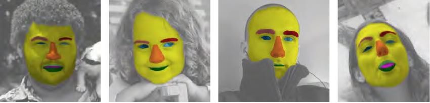
2      Y. Zhou, X. Hu, B. Zhang

et al. [2] exploit structure of information using trees. They extract features from
superpixels using CNN, combine nearby superpixels with same category recur-
sively.
    As a special case of image parsing, face parsing amounts to labeling each
pixel with eye, nose, mouth and so on. It is a basic task in face image analysis.
Compared with general image parsing, it is simpler since facial parts are regular
and highly structured. Nevertheless, it is still challenging since facial parts are
deformable. For this task, landmark extraction is a common practice. But most
landmark points are not well-defined and it is difficult to encode uncertainty
in landmarks like nose ridge [5]. Segmentation-based methods seem to be more
promising [5][6].
    In the paper, we present a deep learning method for face parsing. Inspired by
the models for general image parsing [3][4], we use multiple CNNs for processing
different scales of the image. To allow the CNNs exchange information, an in-
terlinking layer is designed, which concatenates the feature maps of neighboring
CNNs in the previous layer together after downsampling or upsampling. For this
reason, the proposed model is called interlinked CNN or iCNN for short. The
idea of interlinking multiple CNNs is partially inspired by [7] where multiple
classifiers are interlinked.
    Experiments on a pixel-by-pixel [5] labeling version of the Helen dataset [8]
demonstrate the effectiveness of iCNN compared with existing models.

2     iCNN
The overall structure of the proposed iCNN is illustrated in Fig. 1. Roughly
speaking, it consists of several traditional CNN in parallel, which accept input
in different scales, respectively. These CNNs are labeled CNN-1, CNN-2, ... in
the order of decreasing scale. The hallmark of the iCNN is that the parallel
CNNs interact with each other. From left to right in Fig. 1, the iCNN consists
of alternating convolutional layers and interlinking layers, as well as an output
layer, which are described as follows.

2.1   Convolutional Layers
The convolutional layers are the same as in the traditional CNN, where local
                                                                      (l)
connections and weight sharing are used. For a weight kernel wuvkq , the output
of a unit at (i, j) in the l-th layer is
                                C X P1 X P2
                                                                    !
                     (l)                     (l)   (l−1)
                               X
                    yijq = f                wuvkq yi+u,j+v,k + b(l)         (1)
                            k=1 u=1 v=1

where P1 and P2 denote the size of the weight kernel in the feature map, C
denotes the number of channels in the (l − 1)-th layer, b(l) denotes the bias in
the l-th layer, and f (·) is the activation function. Throughout the paper, tanh
                                                                    (l)
function is used as the activation function. If we use Q kernels wuvkq , that is,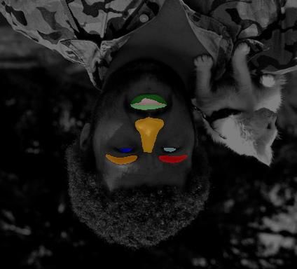
Repeat three times
            3 channels
              {R,G,B}

    CNN-1                                                     24                                        24               2L+8                      L channels        L channels
                                      8 channels                                  8 channels
                                                           channels                                  channels

                  ½ downsampling

    CNN-2                                 16                 48                       16                               16
                                                                                                        40
                                        Chan-              Chan-                    Chan-             Chan-          Chan-
                                         nels               nels                     nels              nels           nels
                  ½ downsampling

    CNN-3

                  ½ downsampling 24 channels       72 channels                 24 channels      56 channels     24 channels

    CNN-4
                                                                                                                         (L: the number of label channels)

                                   32 channels     56 channels                 32 channels

            Input layer            Convolutional       Interlinking            Convolutional   Interlinking     Convolutional                Convolutional      Output layer
                                       layer              layer                    layer          layer             layer                        layer

Fig. 1. The structure of the iCNN. Black solid arrows: convolution and nonlinear transformation as described in (1). Black dotted arrow:
convolution. Black open arrow: softmax. Green arrows: downsampling (mean pooling). Black dashed arrows: pass the feature maps to
the next layer. Blue arrows: downsampling (max pooling) the feature maps and pass them to the next layer. Yellow arrows: upsampling
                                                                                                                                                                                  iCNN for Face Parsing

(nearest neighbor) the feature maps and pass them to the next layer. Best viewed in color.
                                                                                                                                                                                  3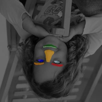
4      Y. Zhou, X. Hu, B. Zhang

q = 1, . . . , Q, then a total number of Q feature maps (the q-th feature map
               (l)
consists of yijq for all i, j) will be obtained in the l-th layer.
    The operation in the bracket in (1) can be implemented by tensor convolution.
The surrounding of feature maps in the (l − 1)-th layer are padded with zeroes
such that after convolution and activation the resulting feature maps in the l-th
layer has the same size in the first two dimensions as the feature maps in the
(l − 1)-th layer.

2.2   Interlinking Layers
In conventional CNN [9][10], there are downsampling layers which perform local
max pooling or average pooling. They can realize shift invariance, which is im-
portant for pattern recognition. Downsampling reduces the size of feature maps.
This is not a problem for pattern recognition (instead it is preferred because
it reduces the computational burden in subsequent layers), but becomes prob-
lematic for scene parsing if an end-to-end model is desired. The output of an
end-to-end model should have the same size as the input image in the first two
dimensions because we have to label every pixel. Considering this requirement,
we do not perform downsampling in the first CNN (top row in Fig. 1). The other
CNNs (other rows in Fig. 1) process the input in smaller scales, and we do not
perform downsampling in their own previous feature maps, either (black dashed
arrows in Fig. 1).
    These parallel CNNs process different scales of the input, which contain dif-
ferent levels of fine to coarse information. To let each CNN utilize multi-scale
information, a special layer is designed. Consider CNN-k. In this layer, the fea-
ture maps from its own previous layer and those from the previous layer of
CNN-(k − 1) and CNN-(k + 1) are concatenated. But the three types of fea-
ture maps cannot be concatenated directly because they have different sizes in
the first two dimensions: those from CNN-(k − 1) are larger than those from
CNN-k and those from CNN-(k + 1) are smaller than those from CNN-k. Our
strategy is to downsample those from CNN-(k − 1) and upsample those from
CNN-(k + 1) such that they have the same size as those from CNN-k in the first
two dimensions. Max pooling is used for downsampling and nearest neighbor
interpolation is used for upsampling. By performing downsampling/upsampling
and then concatenation, we have interlinked the parallel CNNs.

2.3   Output Integration
It has been seen that after either the convolutional layer or interlinking layer,
the size of the feature maps of each CNN in the first two dimensions do not
change. Only CNN-1’s feature maps have the same size as the output tensor in
the first two dimensions. To utilize the information of other CNNs, we perform
the following steps for k = 4, 3, 2 in sequel:
1. upsample CNN-k’s final feature maps to match the size of CNN-(k − 1)’s
   feature maps in the first two dimensions,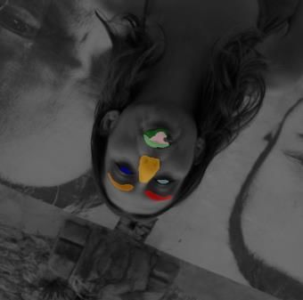
iCNN for Face Parsing         5

 2. concatenate these feature maps with those from CNN-(k − 1), and
 3. perform convolution and nonlinear transformation using (1) to obtain a
    bunch of CNN-(k − 1)’s final feature maps.

After these operations, an additional convolutional layer without nonlinear trans-
formation is used in CNN-1 with L feature maps, where L denotes the number
of different labels. See Fig. 1 for illustration.

2.4   Output Layer

Only CNN-1 has a softmax layer in the end, which output the labels of each
pixel. The output is a 3D tensor with the first two dimensions corresponding to
the input image and the third dimension corresponding to the labels. At each
location of the pixel, the one-hot representation is used for labels, that is, there is
only one element equal to one and others equal to zero along the third dimension.

2.5   Training

The cross-entropy function is used as the loss function. Same as other CNNs,
any minimization technique can be used. Stochastic gradient descend is used in
this project.

2.6   Parameter Setting

For this particular application, the input image has a size of either 64 × 64 or
80 × 80. There are two stages in the proposed face parsing pipeline where in
the first stage the entire image is resized (downsampling) to 64 × 64 and in the
second stage 64 × 64 and 80 × 80 patches are extracted in the original image to
cover the eye/nose/eyebrow and the mouth, respectively. See the next section
for details. For RGB images, the input has three channels. The input image is
then downsampled to 1/2, 1/4 and 1/8 size using a 2 × 2 mean pooling. In all
convolutional layers and all CNNs, the size of the receptive field is set to 5 × 5
(the first two dimensions) except in the last convolutional layer of CNN-1 (the
black dotted arrow) where 9 × 9 is used.

3     Face Parsing with iCNNs

Usually a face image for parsing is large, e.g., the images of Helen dataset [8]
for this task are of the size 256 × 256 [5]. If we input such large images to the
proposed iCNN, both training and testing are slow. To speed up the process we
separate the face parsing procedure into two stages, and both stages use iCNN.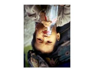
6         Y. Zhou, X. Hu, B. Zhang

3.1     Stage 1: Facial Parts Localization
The goal of this stage is to localize the facial parts including the eyes, nose
and so on with iCNN. Note that we do not label the Face Skin part in this
project, since it has a large area, which is unsuitable for the proposed iCNN to
process. The input image is preprocessed by subtracting the mean and dividing
the norm. The input image as well as its label map is resized to 64 × 64 in the
first two dimensions (both the input image and the output map are 3D tensors)
by downsampling. The output tensor has 9 channels corresponding to the label
maps of background, left eyebrow, left eye, right eyebrow, right eye, nose, upper
lip, inner mouth and lower lip, respectively (Fig. 2). Except the first label map
(background), each median axis of the label map is calculated, and scaled back
to original image to obtain the estimation of the part location. For mouth related
parts (upper lips, inner mouth, lower lips), a shared median axis is calculated.
For the first five parts, 64 × 64 patches are extracted from the original input face
image. For mouth-related parts, a 80 × 80 patch is extracted.

                       iCNN

    64x64 RGB
      image

                                      64x64 RGB Patches                    80x80 RGB Patch

                                                                              iCNN
                 Map results to
                 original image

Fig. 2. The pipeline for face parsing. In the first stage, the entire image is resized to
64 × 64 with aspect ratio kept. It is input to an iCNN and obtain ten label maps where
the first is the background and the others are facial components. The median point
of each component except the two lips and in-mouth is calculated. Since the lips and
in-mouth are processed together, these three parts are first merged together and then
a joint median point is calculated. A 64 × 64 or 80 × 80 patch is extracted around the
median point. In the second stage, with mirroring operation (right eye and eyebrows
flipped), six small parts are processed by four iCNNs to get exact segmentation at the
pixel level. Best viewed in color.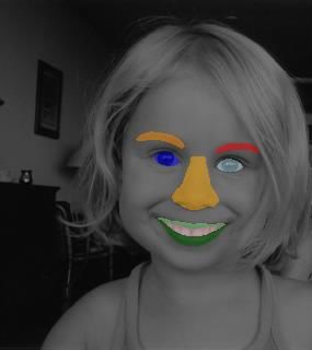
iCNN for Face Parsing        7

3.2   Stage 2: Fine Labeling
In the previous stage, we have extracted the five 64 × 64 patches and one 80 × 80
patch from the original image. Then we use four iCNNs to predict the labels of
the pixels in each patch (Fig. 2). The four iCNNs are used for predicting eye-
brows, eyes, nose, and mouth components, respectively. Note that one iCNN is
used for predicting both left eyebrow and right eyebrow. Since the left eyebrow
and right eyebrow are symmetric, during training the image patches of right eye-
brows are flipped and combined with image patches of left eyebrows. Therefore
this iCNN has only one label map in the output. In testing, the predicted label
maps of right eyebrows are flipped back. Similarly, one iCNN is used for predict-
ing both left eye and right eye. The iCNN for the nose has only one label map
in the output and the iCNN for the mouth components has three label maps.

4     Experiments
4.1   Dataset
The Helen dataset [8] is used for evaluation of the proposed model, which has
2330 face images with dense sampled, manually-annotated contours around the
eyes, eyebrows, nose, outer lips, inner lips and jawline. It is originally designed
as a landmark detection benchmark database. Smith et al. [5] provides a resized
and roughly aligned pixel-level ground truth data to benchmark the face parsing
problem. It generates ground truth eye, eyebrow, nose, inside mouth, upper lip
and lower lip segments automatically by using the manually-annotated contours
as segment boundaries. Some examples of Helen are shown in Fig. 3, where the
first line is the original database images with annotations, and second line is the
processed pixel-based labeling for parsing.

Fig. 3. Example images (top) and corresponding labels (bottom) of the Helen dataset.
Best viewed in color.

   We use the same training, testing and validation partition as in [5]. The dense
annotated data is separated into 3 parts: 2000 images for training, 230 images for
8 Y. Zhou, X. Hu, B. Zhang
validation, and 100 images for testing. The validation set is used to test whether
model is converged.
4.2 Training and Testing
We train the iCNNs in stages 1 and 2 separately. For stage 1, the entire training
images, as well as the corresponding ground truth label maps, are resized to
64 × 64 with aspect ratio kept. For stage 2, the training data are 64 × 64 or
80×80 patches extracted from the original 256×256 training images (see Section
3.1). The corresponding ground truth label maps are extracted from the original
256 × 256 ground truth label maps.
Stochastic gradient descent is used as the training algorithm. Since the num-
ber of images is small compared to number of parameters, to prevent overfitting
and enhance our model, data argumentation is used. During stochastic gradient
descent, a random 15◦ rotation, 0.9∼1.1x scaling, and −10∼10 pixels shifting in
each direction are applied to each input every time when it enters the model.
In Stage 2, by visualizing the feature maps, we find that in the last convolu-
tional layer of CNN-1 among the L feature maps there is a feature map, denote
dy B, corresponding to the background part. We find that modulating this fea-
ture map by βB + β0 can enhance the prediction accuracy. For each facial part,
β and β0 are obtained by maximizing the F-measure [5] on the validation set
using the L-BFGS-B algorithm offered by SciPy, an open-source software.
For testing, each image undergoes stages 1 and 2 in sequel. Only the predicted
labels in stage 2 are used for evaluation of the results.
All codes are written in Theano [11] and Pylearn2 [12].
4.3 Results
The evaluation metric is the F-measure used in [5]. From Table 11 , it is seen
that for most facial parts, iCNNs obtain the highest scores. Note that in our
training data, the labels of Face Skin area are not used. As we can see in the
table, this area is usually a high-score term for most methods, and omitting it
will in no way enhance the overall performance of iCNNs. Even though, iCNNs
achieves higher overall score than existing models. Some example labeling results
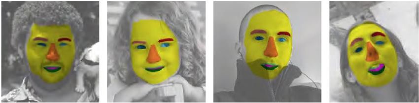
are shown in Fig. 4 along with the results obtained in [5].
5 Concluding Remarks
We propose an interlinked CNN (iCNN), where multiple CNNs process different
levels of details of the input, respectively. Compared with traditional CNNs it
features interlinked layers which not only allow the information flow from fine
level to coarse level but also allow the information flow from coarse level to flow
to the fine level. For face parsing, a two-stage pipeline is designed based on the
1
The results of iCNN are incorrect in our ISNN2015 paper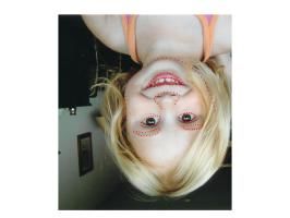
iCNN for Face Parsing 9
Table 1. Comparison with other models (F-Measure)
Model Eye Eyebrow Nose In mouth Upper lip Lower lip Mouth (all) Face Skin Overall
[13] 0.533 n/a n/a 0.425 0.472 0.455 0.687 n/a n/a
[14] 0.679 0.598 0.890 0.600 0.579 0.579 0.769 n/a 0.733
[15] 0.770 0.640 0.843 0.601 0.650 0.618 0.742 0.886 0.738
[16] 0.743 0.681 0.889 0.545 0.568 0.599 0.789 n/a 0.746
[5] 0.785 0.722 0.922 0.713 0.651 0.700 0.857 0.882 0.804
iCNNs 0.778 0.863 0.920 0.777 0.824 0.808 0.889 n/a 0.845
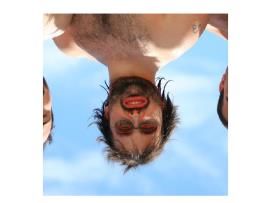
Fig. 4. Labeling results on several example images obtained using the method in [5]
(top) and the proposed method in this paper (middle). The bottom shows the ground
truth labels. Best viewed in color.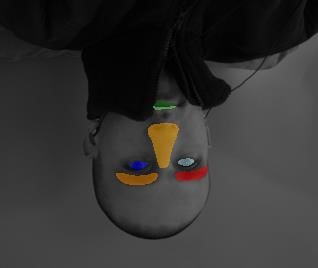
10      Y. Zhou, X. Hu, B. Zhang

proposed iCNN. In the first stage an iCNN is used for facial part localization,
and in the second stage four iCNN are used for pixel labeling. The pipeline does
not involve any feature extraction step and can predict labels from raw pixels.
Experimental results have validated the effectiveness of the proposed method.
    Though this paper focuses on face parsing, the proposed iCNN is not re-
stricted to this particular application. It may be useful for other computer vision
applications such as general image parsing and object detection.

Acknowledgement
The first author would like to thank Megvii Inc. for providing the computing fa-
cilities. This work was supported in part by the National Basic Research Program
(973 Program) of China under Grant 2012CB316301 and Grant 2013CB329403,
in part by the National Natural Science Foundation of China under Grant
61273023, Grant 91420201, and Grant 61332007, in part by the Natural Sci-
ence Foundation of Beijing under Grant 4132046.

References
1. Tu, Z., Chen, X., Yuille, A.L., Zhu, S.C.: Image Parsing: Unifying Segmentation,
   Detection, and Recognition. International Journal of Computer Vision 63, 113-140
   (2005)
2. Socher, R., Lin, C.C., Manning, C., Ng, A.Y.: Parsing Natural Scenes and Natural
   Languages with Recursive Neural Networks. In: ICML, pp. 129-136 (2011)
3. Farabet, C., Couprie, C., Najman, L., LeCun, Y.: Learning Hierarchical Features for
   Scene Labeling. IEEE Transactions on Pattern Analysis and Machine Intelligence
   35, 1915-1929 (2013)
4. Pinheiro, P., Collobert, R.: Recurrent Convolutional Neural Networks for Scene
   Labeling. In: ICML, pp. 82-90 (2014)
5. Smith, B.M., Zhang, L., Brandt, J., Lin, Z., Yang, J.: Exemplar-based Face Parsing.
   In: CVPR, PP. 3484-3491 (2013)
6. Luo, P., Wang, X., Tang, X.: Hierarchical Face Parsing via Deep Learning. In:
   CVPR, pp. 2480-2487 (2012)
7. Seyedhosseini, M., Sajjadi, M., Tasdizen, T.: Image Segmentation with Cascaded
   Hierarchical Models and Logistic Dsjunctive Normal Networks. In: ICCV, pp. 2168-
   2175 (2013)
8. Le, V., Brandt, J., Lin, Z., Bourdev, L., Huang, T.S.: Interactive Facial Feature
   Localization. ECCV, pp. 679-692 (2012)
9. LeCun, Y., Bottou, L., Bengio, Y., Haffner, P.: Gradient Based Learning Applied
   to Document Recognition. Proceedings of the IEEE 86(11), 2278C2324 (1998)
10. Krizhevsky, A., Sutskever, I., Hinton, G. E.: Imagenet Classification with Deep
   Convolutional Neural Networks. In Advances in Neural Information Processing Sys-
   tems (NIPS), pp. 1097C1105, (2012)
11. Bergstra, J., Breuleux, O., Bastien, F., Lamblin, P., Pascanu, R., Desjardins, G.,
   Turian, J., Warde-Farley, D., Bengio, Y.: Theano: A CPU and GPU Math Expres-
   sion Compiler. In: Procesedings of the Python for Scientific Computing Conference
   (SciPy) (2010)
iCNN for Face Parsing 11 12. Goodfellow, I.J., Warde-Farley, D., Lamblin, P., Dumoulin, V., Mirza, M., Pascanu, R., Bergstra, J., Bastien, F., Bengio, Y.: Pylearn2: a Machine Learning Research Library. arXiv preprint arXiv:1308.4214 (2013) 13. Zhu, X., Ramanan, D.: Face Detection, Pose Estimation and Landmark Localiza- tion in the Wild. In: CVPR (2012) 14. Saragih, J. M., Lucey, S., Cohn, J. F.: Face Alignment Throughsubspace Con- strained Mean-Shifts. In: CVPR (2009) 15. Liu, C., Yuen, J., Torralba, A.: Nonparametric Scene Parsing via Label Transfer. IEEE Transactions on Pattern Analysis and Machine Intelligence 33(12), 2368-2382 (2011) 16. Gu, L., Kanade, T.: A Generative Shape Regularization Model for Robust Face Alignment. In: ECCV (2008)
You can also read