FULLY CONSTRAINED LEAST SQUARES LINEAR SPECTRAL UNMIXING OF
←
→
Page content transcription
If your browser does not render page correctly, please read the page content below
FULLY CONSTRAINED LEAST SQUARES LINEAR SPECTRAL UNMIXING OF
                             THE SCREAM (VERSO, 1893)

                        Hilda Deborah                                              Magnus Orn Ulfarsson, Jakob Sigurdsson

         Department of Computer Science,                                             Department of Electrical and Computer
        Norwegian University of Science and                                            Engineering, University of Iceland
           Technology, Gjøvik, Norway                                                         Reykjavik, Iceland

                             ABSTRACT                                          or unmixing tasks. A classification task is when the aim is
                                                                               to identify the main pigments present in a painting. If the
Taking insights from the remote sensing field, in the recent
                                                                               estimation of their proportion is also required, then the task
decade, the advantages of hyperspectral imaging technology
                                                                               becomes that of an unmixing.
has been exploited for painting conservation. The estimation
of pigment proportion in painting is a challenge that is due to                     Hyperspectral unmixing (HU) is an active research area
the highly mixed nature of the paint layers, usually requiring                 in the field of remote sensing. It formulates that an observed
to take into account the law of mixing colorants in turbid me-                 spectral signature, typically originating from a single pixel, is
dia. Having knowledge of some pigments and paint layers of                     of either micro- or macroscopic material mixtures and multi-
the reverse side of The Scream (1893), in this study, we are                   ple scattering [7]. In remote sensing, due to the low resolu-
exploring the feasibility of using a more simple linear model                  tion of the sensor, linear HU can be used since a macroscopic
for its unmixing. The obtained results are promising, despite                  fashion (optical) of the mixture can be assumed. In painting
the simplicity of the mathematical model.                                      conservation, the resolution of a pixel is very high, since the
                                                                               distance between the object of interest and the sensor is sig-
    Index Terms— hyperspectral images, spectral unmixing,                      nificantly closer compared to that in the remote sensing setup.
fully constrained least squares, cultural heritage application                 Additionally, the mixing law for when different wet paints are
                                                                               mixed is different from that of an optical mixing in the atmo-
                       1. INTRODUCTION                                         sphere. Kubelka-Munk (K-M) theory is the mixing law of
                                                                               colorants that are largely used in the HU of paintings [5, 6].
The identification of an artist’s material of a painting is tradi-                  K-M theory expresses the relationship between absorption
tionally carried out using micro-destructive techniques, e.g.,                 and scattering coefficients of incident lights in intensely light
X-ray fluorescence (XRF) and Fourier-transform infrared                        scattering materials or, what is called, turbid media [8]. How-
spectroscopy (FTIR) [1]. Despite allowing to identify pig-                     ever, it is mathematically complex, making it unsuitable for
ments, dyes, and organic components present in the painting,                   many applications. This has lead to its simplifications which,
they are only point-analysis. Hyperspectral imaging (HSI),                     nevertheless, still have their challenges. They are known to
which captures both spatial and spectral information, offers                   be restrictive and their shortcomings and limitations have also
a complementary non-invasive technique to the field of con-                    been identified [9, 10].
servation. With the characteristic wavelengths of paints lying                      For paintings that have been previously analyzed using
in the visible and near-infrared spectral ranges [2], HSI can                  the traditional point-wise techniques, we have what is analo-
provide an analysis of pigments for the surface of a painting.                 gous to ground truth in the remote sensing context. This is
    The use of spectral imaging for painting conservation                      available for The Scream (1893) by Edvard Munch [11, 12],
started in the early 90s [3], aimed at providing more accurate                 for which we have also previously mapped the presence of its
documentation of cultural heritage paintings. In the recent                    main pigments on the entire surface of the painting [4]. Ex-
decade, we can find works exploiting the use and advantages                    ploiting the knowledge of the particular characteristics of its
of HSI to provide, e.g., pigment and constituent maps, show-                   reverse side, in this study, we are exploring the feasibility of
ing their presence [4] and also their estimated proportion                     using the linear spectral mixture analysis approach. Details of
or concentration in a mixture [5, 6]. From a computational                     the said characteristics, the methods, and our justification of
point of view, these works can be categorized as classification                its use can be found in Section 2. Some experimental results
    This work is supported by FRIPRO FRINATEK Metrological texture
                                                                               and analysis can be found in Section 3, followed by a conclu-
analysis for hyperspectral images (projectnr. 274881) funded by the Research   sion in Section 4. Frequently used mathematical notations are
Council of Norway.                                                             also provided for ease of reading in Table 1.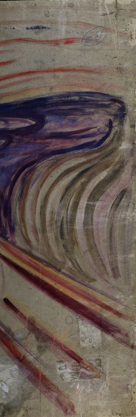
Table 1: Frequently used mathematical notations.
×M
Y Image vector Y = [ypT ], Y ∈ RP + , where
M ×1
yp ∈ R+ is the spectrum at pixel p
A Spectral signatures of known pigments A = [ar ],
×R ×1
A ∈ RM + , ar ∈ RM +
×R
S Proportion vector S = [sp ], S ∈ RP + , sp ∈
1×R
R+
1r , 1p Vector of ones of size R × 1 and P × 1
M Number of spectral bands
P, p Number of pixels and pixel index
R, r Number of known pigments and their index
2. MATERIALS AND METHODS
2.1. Target painting
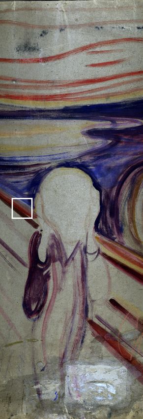
The target painting for this study is the reverse side (verso) Fig. 1: Three hyperspectral cutouts of the reverse side (verso)
of the painted version of The Scream (tempera/ crayon/ oil, of The Scream (1893).
Woll 333) from 1893, owned by the National Museum of Art,
Architecture and Design (NM) in Oslo, Norway [13]. Due to ments present in the painting is required. In this case, this
the size of the painting and the acquisition setup, the painting information is obtained from previous studies, where the main
had to be scanned as three overlapping cutouts (Fig. 1). After pigments have been identified in several points of the paint-
a preprocessing, each cutout is of varying widths and heights ing [11, 12]. Using them as guidance, spectral reflectances of
around 1400×4680 pixels. Spectrally, it has 160 bands from the identified pigments can therefore be extracted from the
approximately 414.62 to 992.50 nm, in 3.63 nm intervals. hyperspectral image in order to build a matrix A containing
Due to the noise level at the first five bands, only 155 spectral the signatures of the pigments.
bands starting from 432.80 nm are considered. For a linear unmixing approach to provide reliable and
In an interview with a conservator from the NM [14], it directly interpretable estimation of pigment proportion S, two
was mentioned that Munch very rarely mixed the paints in constraints must be imposed. They are the abundance non-
the palette, but rather directly onto the cardboard support of negativity (ANC) and sum-to-one (ASC) constraints [15],
this painting. It was further explained the technique he often
R
used was brushing one paint thinly across another, resulting X
in a third color that is optically mixed. And as what can also spr ≥ 0, 1 ≤ r ≤ R; spr = 1.
r=1
be observed in the reverse side of the painting in Fig. 1, there
are many strokes of clean or unmixed colors. There are also These constraints allow embedding the physical aspects of
what is called the scumble effects, i.e., a perceptual effect that materials into the algorithm. ANC says that the estimated
is due to the translucent colors lying across each other. An- proportion for each pigment must be a positive fraction, while
other important aspect of the painting that will be useful in ASC makes sure that the cumulative proportion of a single-
the unmixing task is the cardboard support. It was said that pixel p does not go above 100%.
there was no proper preparation for the cardboard. There is no In a least squares linear unmixing, we consider a pixel yp
ground layer aside from gelatin that was already on the card- to be modeled as a linear combination of spectral signatures
board itself. This means that for a thin layer of paint or pig- of known pigments Asp and an additive noise term p ,
ment, the spectral reflectance will be that of an optical mixing
with the reflectance of the cardboard support. yp = Asp + p , p = 1, . . . , P.
Then, consider the optimization problem,
2.2. Fully constrained least squares unmixing
P
1X
The characteristics of The Scream (1893), i.e., with many J = min kyp − Asp k2 + λ1 kS1r − 1p k2 + λ2 kSkq ,
S 2 p=1
clean colors and scumble effects, justify the use of a more
simple unmixing algorithm, i.e., fully constrained least P X
X R
squares (FCLS) linear spectral unmixing. In order to use where kSkq = sqpr , 0 < q < 1.
the algorithm, a priori knowledge of the signatures of pig- p=1 r=1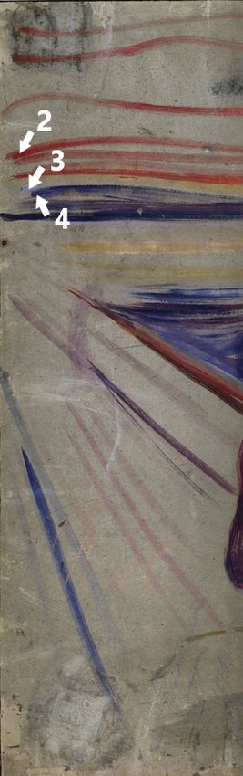
The first term in J enforces fidelity, the second encourages             Table 2: Known pigments used in this study. Sample num-
ASC, and the third acts as a sparsity term. Considering the              bers in parentheses correspond to physical samples studied
whole image vector Y, the function can be written as,                    and analyzed in Ref. [11].

               1                                                          Sample      Colour    Main pigments found
  J = min        kY − SAT k2F + λ1 kS1r − 1p k2 + λ2 kSkq .
         S     2
                                                                              1        -        Cardboard support
To optimize J, the steepest descent method will be used,                   2 (33)     Red       Vermilion
where its derivative w.r.t S is,                                           3 (35)     White     LW mixture: Lead white, zinc white
                                                                           4 (34)     Blue      UB mixture: Ultramarine blue, lead
∂J
   = SAT A − YA + λ2 qkSkq−1 + λ1 S1r 1Tr − λ1 1p 1Tr .                                         white, barites
∂S
The (element-wise) steepest descent method for each iteration
k is given by,

      s(k+1)
       pr    = s(k)   (k)
                pr − ηpr [(S
                            (k) T
                               A A)pr − (YA)pr +
                  λ2 q(s(k)
                        pr )
                             q−1
                                 + λ1 (S(k) 1r 1Tr )pr − λ1 ].

The step size ηpr is allowed to change at each k,
                                      (k)
 (k)                                 spr
ηpr  =                               (k)
                                                                  .
         [(S(k) AT A)pr + λ2 q(spr )q−1 + λ1 (S(k) 1r 1Tr )pr ]          Fig. 2: Spectral reflectances of the samples given in Table 2.
Finally, the update rule can be written as,                              Colors of the spectra are representative of the main pigments.

                               (k)
                              spr [(YA)pr + λ1 ]
s(k+1)
 pr    =                               (k)
                                                                      . mixed pigments in this subset are only variations of samples
             [(S(k) AT A)pr + λ2 q(spr )q−1 + λ1 (S(k) 1r 1Tr )pr ]     1-4. The estimated proportion in different pixels will vary,
                                                                        but no other pigments are expected on the surface, which will
With regards to ANC, it is possible to show that the sequence
                                                                        contribute to a significantly larger reconstruction error e =
of cost function values this algorithm yield is non-negative
                                                                        kY − SAT k2F .
[16]. Note that the method relates to refs. [16, 17], written for
                                                                             The unmixing results can be observed in Fig. 3. The pro-
non-negative matrix factorization setting.
                                                                        portion maps for each sample in Fig. 3c-3f provide reason-
                                                                        able results agreeing with a quick visual observation on the
2.3. Spectral library of pure and mixed pigments                        target image. The map for the cardboard support (Fig. 3c)
Information of the main pigments present in the three loca-             correctly shows where the cardboard is exposed, without any
tions pointed by white arrows in Fig. 1 is available [11].              superposing paint layer. Its combination with the vermilion
Details of their corresponding pigments are provided in Ta-             map (Fig. 3d) is also able to show where the vermilion layer
ble 2. Additionally, knowing that most of the surfaces are              is thinner and more translucent, showing the cardboard layer
not covered by pigments, a signature of the cardboard sup-              beneath. The map for the LW mixture correctly provides a
port will also be used in the spectral library. Finally, spec-          high proportion in the brushstroke where sample 3 was taken
tral reflectances of these four samples are obtained from, first,       from. However, it also shows that the LW mixture is found
averaging a 2 × 2 window and, then, smoothing them using                where the cardboard support is supposedly exposed. This
Savitzky-Golay filter [18] of window length 7 and polynomial            can be explained through the high similarity between spec-
order 2. The resulting spectral library can be seen in Fig. 2.          tral reflectances of sample 1 (cardboard) and 3 (LW mixture),
                                                                        see Fig. 2. This is understandable and expected since in the
                                                                        VNIR spectral range, the shape of cardboard and white pig-
               3. RESULTS AND DISCUSSION                                ments spectra are difficult to differentiate. It can be easily
                                                                        solved by incorporating SWIR spectral ranges encompassing
3.1. Evaluation using subsets containing the samples
                                                                        cellulose absorption bands.
To evaluate the feasibility of using FCLS for this painting, a               Fig. 3f shows a high proportion of UB mixture in the
subset of size 300×300 pixels is used, as well as the following         brushstrokes area where sample 4 was taken from. However,
tuning parameters λ1 = 1300, λ2 = 23, q = 0.5. It contains              this area also generates relatively high e in Fig. 3b. The spec-
the location of the samples in Fig. 1. Closely observing the            tra of three pixels with the highest e from this area are shown
subset through Fig. 3a, it is almost certain that pure and/ or          in Fig. 5. The spectrum corresponding to e = 0.35 has a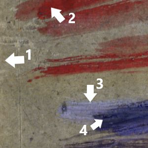
(a) Target subset    (b) Reconstruction error     (c) Cardboard     (d) Vermilion      (e) LW mixture         (f) UB mixture

Fig. 3: Results for a subset of verso (L) containing the origin of samples 1–4 (Table 2). Subfigures (c)-(f) provide the estimated
proportion of each samples and are of identical dynamic ranges, i.e., 0–1.

    (a) Target subset      (b) Cardboard           (c) Vermilion     (d) LW mixture      (e) UB mixture       (f) Unknown mixture

    Fig. 4: Results for a subset containing paint layers supposedly of the samples in Table 2 and another unknown mixture.

                                                                     these known pigments are present are annotated in the target
                                                                     image. There is also an unknown red-brownish paint layer
                                                                     which was not recognized as vermilion in Ref. [4], giving a
                                                                     higher e compared to the rest. A quick experiment using only
                                                                     the spectral library in Table 2 also supports the mapping study.
                                                                         Adding a signature of the unknown layer to the spectral
                                                                     library, the unmixing is carried out, resulting in maps in Fig.
                                                                     4. As previously, the proportion map for cardboard (Fig. 4b)
                                                                     is able to identify the exposed support and where the paint
Fig. 5: Three pixels with highest reconstruction error e, lo-        layer above it is thin and translucent. The map for vermil-
cated in brushtroke areas with high proportion of UB mixture.        ion (Fig. 4c) agrees with the result in Ref. [4]. The issue
                                                                     with the LW mixture being recognized where the cardboard
                                                                     is exposed remains a challenge for this subset. However, the
peak at around 450 nm, which does not exist in the signature         map (Fig. 4d) shows a high proportion of the mixture in a
of sample 4 (UB mixture). This could mean that there is an           location agreeing with our hypothesis. The map for the UB
unknown blue pigment in the mixture. The two other spectra           mixture (Fig. 4e) also agrees with the result in Ref. [4], ex-
are almost identical in shape with the spectrum of sample 4,         cept for areas where the mixture is darker in color. Finally,
only lower in intensity. FCLS deems them to be composed of           for the unknown mixture, the map is giving nearly 100% in
nearly 100% sample 4. The reconstruction error is then due           the brushstroke area where the signature is taken from. It
to the ASC constraint imposed on the algorithm. To go very           also says that the top right area of the subset consists of this
close to the spectrum of sample 4, it would require spr ≥ 1.         red-brownish pigment, which is likely a false-positive since it
                                                                     would most probably be a UB mixture [4]. This problem can
3.2. Unmixing of image subset of unknown paint layers                be attributed to the use of F-norm in the cost function, which
                                                                     takes into account intensity differences between spectra while
Using the knowledge from a previous mapping study [4], an-           neglecting the shape information [19]. Intensity difference is
other subset is chosen as a target. Its location is approximately    necessary to calculate the proportion, however, shape differ-
within the white square of the second image in Fig. 1. From          ence captures the characteristics of individual pigments. For
that study we know that this subset contains vermilion and           example, a mixture of red pigments would not typically have
UB mixture. From a visual observation of Fig. 4a, it is possi-       a peak around 450 nm, since it is usually the characteristic of
ble that LW mixture is also present. Our hypothesis of where         blue pigments. This information of peak location will be well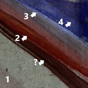
accounted for in the shape difference, instead of the intensity.     [7] J. M. Bioucas-Dias, A. Plaza et al., “Hyperspectral un-
                                                                         mixing overview: Geometrical, statistical, and sparse
        4. CONCLUSION AND FUTURE WORK                                    regression-based approaches,” IEEE J Sel Top Appl
                                                                         Earth Obs Remote Sens, vol. 5, no. 2, pp. 354–379,
The hyperspectral unmixing of paintings into their pigments              2012.
is a challenge due to the complex nature of spectral mix-            [8] H. Yang, S. Zhu, and N. Pan, “On the Kubelka-
ing in turbid media, e.g., paint layers. Kubelka-Munk col-               Munk single-constant/two-constant theories,” Text Res
orant mixing law is typically incorporated in the model. How-            J, vol. 80, no. 3, pp. 263–270, 2010.
ever, it is mathematically complex and its simplifications are       [9] R. S. Berns and M. Mohammadi, “Single-constant sim-
also known to be restrictive. The reverse side of The Scream             plification of Kubelka-Munk turbid-media theory for
(1893) is composed of many clean colors and scumble effect,              paint systems–A review,” Color Res Appl, vol. 32, no. 3,
enabling us to assume that the painting can be modeled us-               pp. 201–207, 2007.
ing a fully-constrained least-squares linear mixing model. A        [10] A. K. R. Choudhury, “Instrumental colourant formula-
spectral library of known pigments was also built using a few            tion,” in Principles of Colour and Appearance Measure-
ground truth information available from previous studies.                ment. Woodhead Publishing, 2015, pp. 117–173.
    The results obtained in this study are promising, agreeing      [11] B. Singer, T. E. Aslaksby et al., “Investigation of ma-
with a previous pigment mapping study. A number of limita-               terials used by Edvard Munch,” Stud Conserv, vol. 55,
tions have been identified, suggesting some improvements for             no. 4, pp. 274–292, 2010.
future works. A separate study can be carried out to build an       [12] I. C. A. Sandu, T. Ford et al., “The ”Scream” by Ed-
optimal spectral library, guided by the knowledge of the avail-          vard Munch - Same motif, different colours, differ-
able ground truth. More signatures of pigments beyond the                ent techniques and approaches – A novel non-invasive
ground truth would also be necessary, possibly using informa-            comparative study of two of its versions,” in 5th Inter-
tion from the front side of the painting. It would also be inter-        national Congress on Chemistry for Cultural Heritage
esting to compare the results with an algorithm that uses, e.g.,         (ChemCH2018), 2018.
spectral angle distance in place of the F-norm, in order to ac-     [13] T. E. Aslaksby, “Edvard Munch’s painting The Scream
count for individual pigment characteristics. Finally, a com-            (1893): Notes on technique, materials and condition,”
parison with the widely used Kubelka-Munk theory would be                in Public paintings by Edvard Munch and some of his
necessary to provide more understanding of when a simpler                contemporaries. Changes and conservation challenges.
mixing model can be employed for the unmixing of paintings.              Archetype Publications, 2015.
                                                                    [14] Exhibition on Screen. (2017) Interview with Trond E.
                                                                         Aslaksby, Conservator, The National Museum in Oslo.
                     5. REFERENCES
                                                                         https://www.youtube.com/watch?v=5QpwoNXel6E.
                                                                    [15] D. C. Heinz and C. I. Chang, “Fully constrained least
 [1] V. Antunes, V. Serrão et al., “Characterization of a pair
                                                                         squares linear spectral mixture analysis method for ma-
     of Goan paintings from the 16th-17th centuries,” Eur
                                                                         terial quantification in hyperspectral imagery,” IEEE
     Phys J Plus, vol. 134, no. 6, p. 262, 2019.
                                                                         Trans Geosci Remote Sens, vol. 39, no. 3, pp. 529–545,
 [2] M. T. Eismann, Hyperspectral remote sensing. SPIE,
                                                                         2001.
     2012.
                                                                    [16] Y. Qian, S. Jia et al., “Hyperspectral unmixing via L1/2
 [3] K. Martinez, “High resolution digital imaging of paint-
                                                                         sparsity-constrained nonnegative matrix factorization,”
     ings: The Vasari Project,” Microcomputers for Informa-
                                                                         IEEE Trans Geosci Remote Sens, vol. 49, no. 11, pp.
     tion Management, vol. 8, no. 4, pp. 277–283, 1991.
                                                                         4282–4297, 2011.
 [4] H. Deborah, S. George, and J. Hardeberg, “Spectral-
                                                                    [17] D. D. Lee and H. S. Seung, “Algorithms for non-
     divergence based pigment discrimination and mapping:
                                                                         negative matrix factorization,” in Proc. 13th Interna-
     A case study on The Scream (1893) by Edvard Munch,”
                                                                         tional Conference on Neural Information Processing
     J. Am. Inst. Conserv., vol. 58, no. 1-2, pp. 90–107, 2019.
                                                                         Systems, 2000, pp. 535–541.
 [5] F. M. Abed and R. S. Berns, “Linear modeling of mod-
                                                                    [18] A. Savitzky and M. J. E. Golay, “Smoothing and differ-
     ern artist paints using a modification of the opaque form
                                                                         entiation of data by simplified least squares procedures,”
     of KubelkaMunk turbid media theory,” Color Res Appl,
                                                                         Anal. Chem, vol. 36, no. 8, pp. 1627–1639, 1964.
     vol. 42, no. 3, pp. 308–315, 2017.
                                                                    [19] H. Deborah, N. Richard, and J. Y. Hardeberg, “A com-
 [6] A. M. N. Taufique and D. W. Messinger, “Hyperspectral
                                                                         prehensive evaluation of spectral distance functions and
     pigment analysis of cultural heritage artifacts using the
                                                                         metrics for hyperspectral image processing,” IEEE J Sel
     opaque form of Kubelka-Munk theory,” in Algorithms,
                                                                         Top Appl Earth Obs Remote Sens, vol. 8, no. 6, pp.
     Technologies, and Applications for Multispectral and
                                                                         3224–3234, 2015.
     Hyperspectral Imagery XXV, vol. 10986. SPIE, 2019,
     pp. 297–307.
You can also read