The Bene ts of Forced Experimentation: Striking Evidence from the London Underground Network
←
→
Page content transcription
If your browser does not render page correctly, please read the page content below
The Bene…ts of Forced Experimentation: Striking
   Evidence from the London Underground Network
          Shaun Larcomy                 Ferdinand Rauchz                 Tim Willemsx

                                       August 29, 2015

                                             Abstract

          We estimate that a signi…cant fraction of commuters on the London underground
      do not travel their optimal route. Consequently, a tube strike (which forced many
      commuters to experiment with new routes) taught commuters about the existence
      of superior journeys – bringing about lasting changes in behavior. This e¤ect is
      stronger for commuters who live in areas where the tube map is more distorted,
      thereby pointing towards the importance of informational imperfections. We argue
      that the information produced by the strike improved network-e¢ ciency. Search
      costs are unlikely to explain the suboptimal behavior. Instead, individuals seem to
      under-experiment in normal times, as a result of which constraints can be welfare-
      improving.
          JEL-classi…cation: D83, L91, R41
          Key words: Experimentation, Learning, Optimization, Rationality, Search

     Many thanks to Transport for London (especially Dale Campbell and Maeve Clements) for providing
us with the necessary data. We also thank David Cox, Guy Michaels, Jörn-Ste¤en Pischke, Kevin Roberts,
Alastair Young, and participants at the 2015 Workshop on Structural Transformation in St Andrews for
useful comments and discussions. Francesca di Nuzzo provided excellent research assistance.
   y
     Department of Land Economy, University of Cambridge. E-mail: stl25@cam.ac.uk.
   z
     Department of Economics, University of Oxford. E-mail: ferdinand.rauch@economics.ox.ac.uk.
   x
     Nu¢ eld College, Department of Economics, University of Oxford, and Centre for Macroeconomics.
E-mail: tim.willems@economics.ox.ac.uk.

                                                  1
1 Introduction
Do agents make …rst-best choices? Or are they at least able to learn the optimum if
the underlying problem repeats itself over time? Answers to these questions are of great
interest to economists across all …elds, but have also been subject to intense debate.
We present evidence on these questions by analyzing a unique dataset from the London
underground network, which enables us to track individual commuter behavior over time.
In addition to providing detailed information on commuter patterns in a world city
like London, our dataset contains a tube strike. Thanks to the presence of this event,
we can carry out a detailed empirical investigation on the e¤ects of experimentation.
We are able to do this because the strike caused major disruptions on the underground
network on February 5 and 6, 2014. During these days, some (but not all) tube stations
were closed. As a result, we know that certain commuters were forced to experiment
and explore new routes on these days. In this paper, we analyze whether such a (forced)
period of experimentation produces any observable e¤ects that last beyond the duration
of the strike. In other words: when all stations were open again on February 7, did people
switch back to their original paths, or did some of them stick to the alternative route
that they found during the disruption? By a revealed preference-type argument, the
latter possibility would suggest that they prefer the newly discovered alternative to their
old habit – indicating that these commuters failed to …nd their best alternative in the
pre-strike period.
The underlying issue at stake (minimizing commuting time, and time spent on the
tube during rush hour in particular) is an important one, as commuting is well-known to
have a signi…cant negative impact on life-satisfaction: Stutzer and Frey (2008) for example
calculate that reducing total commuting time by 44 minutes a day, is worth about 35%
of average monthly labor income in terms of well-being.1
Despite these signi…cant stakes, we encountered anecdotal evidence suggesting that the
strike produced useful information, bringing about lasting changes in commuter behavior.2
With this paper, we try to analyze the importance of such considerations in a detailed
1
Ahlfeldt et al. (forthcoming) estimate an even greater cost of commuting: they …nd that a 10 minute
commute, reduces utility by 14 percentage points (whereas the utility-based number in Stutzer and Frey
(2008) is 10 percentage points).
2
See e.g. http://www.bbc.co.uk/news/uk-england-london-26037534, where it is noted that "some
commuters have discovered more enjoyable ways of getting to work." That article for example cites a
commuter named Andy, who has experimented by taking the Thames Clipper water bus. He commented:
"It has been …ne, the boat is a great journey. I think I will get the boat back too." Another commuter
(named as Chris Fry) is quoted as saying that "the walk from Liverpool Street was a refreshing change
from the horrors of the Circle Line. I suspect I may permanently switch so I can cut out this, the most
stressful part of my journey."
2manner.
The results of this study will tell us something about the ability of individuals to …nd
optimal paths in networks, as well as on their approach to problem-solving. The latter
issue has been subject to intense debate over many years. While the rational approach
to decision-making has a long history in economics (in particular see contributions by
Rothschild (1974a), Weitzman (1979), Roberts and Weitzman (1981), and Morgan and
Manning (1985) to the literature on optimal search), others have remained skeptical of this
characterization. Simon (1955) for example argued that agents are "satis…cing" rather
than maximizing –meaning that they stop their search-for-the-optimum once they have
reached a satisfactory utility-level and apply rules-of-thumb from that point onward. It
should be noted that although "satis…cing" behavior could imply irrationality, this is not
necessarily so. Subsequent theoretical contributions (like Baumol and Quandt (1964))
have for example shown that such behavior may very well be rational when there are
costs associated with decision-making – thereby anticipating the aforementioned search
literature pioneered by Rothschild (1974a) and Weitzman (1979).3 Baumol and Quandt
(1964) distinguish between "optimal" and "maximal" solutions: the latter refers to the
exact solution, which would be obtained if there were no search costs, while the former
takes such costs into account. Caplin, Dean and Martin (2011) provide experimental
evidence which suggests that the "satis…cing-approach" o¤ers a good characterization of
agents in a laboratory-environment. With this paper, we are able to provide evidence on
this matter by using data generated by a large number of actual consumers, representing
a sizable fraction of London’s full population.
Our results are particularly informative on the inclination of individuals to experiment.
After all, the alternative commute was already available pre-strike and could have been
found beforehand through "voluntary" (as opposed to "forced") experimentation. Many
theoretical papers have pointed out that a certain degree of experimentation is optimal
in settings where information is imperfect,4 but to the best of our knowledge there is
no empirical work analyzing the incidence (as well as the e¤ects) of experimentation
in practice. This paper is able to contribute along this dimension, as we know when
exactly many commuters were experimenting (namely during the strike), while the tube-
environment provides us with a setting in which information is very imperfect. The
3
More recently, Sims’ (2003) theory of rational inattention formalizes a similar idea: in his setup,
decision makers have to allocate their scarce attention over multiple sources of uncertainty, which leads
to deviations from standard "maximizing" behavior. Also see Matejka and McKay (2015) for an extension
of the theory of rational inattention to a discrete-choice setup that characterizes our setting (should I
take route A or route B?).
4
See e.g. Rothschild (1974b), Aghion et al. (1991) and Bolton and Harris (1999).
3distorted nature of the schematic London tube map (which many travelers use to navigate)
makes it di¢ cult for travelers to minimize journey time (Guo, 2011).5 The fact that many
line-characteristics are initially unknown (the line’s crowdedness, the nature of the follow-
up journey to the …nal destination, etc.) plays a complicating role as well.
Thanks to the presence of informational imperfections, our study is also able to add
to the debate on the so-called "Porter-hypothesis". Porter (1991) argued that – when
information is imperfect –exogenously-imposed constraints may help agents to get closer
to their optimum by triggering a period of experimentation and re-optimization. Porter
originally phrased his hypothesis in the context of environmental regulation,6 but the
underlying idea is more general and also applies to the tube-setup considered in this
paper.
Problematically to some, the Porter-hypothesis imposes a great deal of irrationality
on the part of decision-makers: it implies that $10 bills are waiting to be picked up from
the pavement. After all, why would it take an exogenously-imposed constraint to make
agents realize that they were not optimizing beforehand? Why wouldn’t they experiment
voluntarily? As a result, Porter’s hypothesis has been dismissed by many scholars as
being unrealistic – initially mostly on anecdotal grounds (see e.g. Palmer, Oates and
Portney (1995) and Schmalensee (1993)). Subsequently, many studies have tried to test
the theory empirically but, as noted by Porter and Van der Linde (1995) and Ambec
et al. (2014), data limitations make it hard to put Porter’s hypothesis to a proper test
in practice. The fact that measureable progress often takes time to occur makes it for
example di¢ cult to keep "all else equal", while it is also not clear how "an improvement"
is to be de…ned in the …rst place. As a result of these complications, the literature has not
settled upon a consensus with respect to this issue (see e.g. Gray (1987), Ja¤e and Palmer
5
The informational imperfection is beautifully described in The Guardian of April 27, 2015. There it
is written that: "When you …rst move to London it’s very common to quickly gain very detailed, even
intimate knowledge of two or three locales, but not know how they are connected geographically. It’s
not until there’s a Tube strike and you have to cycle or take the bus [...] that you suddenly realise that
places you thought were separated by several sets of escalators and two Tube lines are only 15 minutes
walk apart. It was only last week that one of us realised that Goodge Street is a short walk from Euston
Station." Similarly, Alan Turing once described a friend as "[thinking] of Paris like [...] I would think
of a Riemann surface; he only knew the circles of convergence round every Metro station, and couldn’t
analytically continue from one to another" (Hodges, 2014: 610).
6
Porter stated that tighter environmental standards "do not inevitably hinder competitive advantage
against foreign rivals; indeed, they often enhance it. Tough standards trigger innovation and upgrading".
Similarly, Porter and Van der Linde (1995: 98) claim that environmental regulations can "trigger innova-
tion (...) that may partially or more than fully o¤set the costs of complying with them". This idea goes
back to the notion of "induced innovation", developed in Hicks (1932), and has also been taken beyond
Porter’s original application to environmental regulation (see e.g. Aghion, Dewatripont and Rey (1997)
for a paper that analyzes related issues in a more general setup).
4(1997), Berman and Bui (2001), and Copeland and Taylor (2004)). By analyzing the
revealed behavior of commuters who were faced with a short-lived, temporary constraint
on the London underground network, the present study overcomes many of these problems
(although it may introduce others –a potential concern that we will try to address as we
go along).
Our study is also insightful on the existence, strength, and persistence of habits. As
noted by Wood and Neal (2009), research on habits is important since about 45% of
people’s behavior is repeated on a daily basis. Commuter behavior is an exponent of this.
Along these lines, Goodwin (1977: 95) has for example argued that "the traveler does not
carefully and deliberately calculate anew each morning whether to go to work by car or
bus. Such deliberation is likely to occur only occasionally, probably in response to some
large change in the situation".
Finally, we believe that our paper is the …rst to comprehensively analyze the e¤ects of
a public transport strike. Although there are some earlier studies analyzing disruptions in
transportation networks (see Van Exel and Rietveld (2001) for an overview of this sparse
literature), they tend to rely on survey data –thereby leading to small sample sizes and
preventing a clean comparative analysis of travel patterns before and after the disruption
(Zhu and Levinson, 2011: 19). As we will explain in greater detail in Section 4, the present
study has the entire population of actual travel movements on the London underground
at its disposal, which brings advantages over earlier contributions.
The remainder of this paper is structured as follows. We start by providing background
information on the London underground network in Section 2. Subsequently, Section 3
describes the tube strike that took place in February 2014, after which we discuss our
dataset in Section 4. To motive certain choices in our empirical exercise, we provide
some notable descriptive statistics in Section 5 (which may also be of general interest and
relevance), after which Section 6 continues by describing our method. We then present
our analysis of the e¤ects of the strike in Section 7, after which Section 8 interprets our
results. Section 9 concludes.
2 The London underground network
Given that we are going to derive most of our information from a strike that a¤ected
the London underground network, we use this section to describe this network in some
necessary detail.
Over the sample period considered in this paper (January 19 to February 15, 2014),
5the London underground network consisted of 11 di¤erent lines, connecting 270 di¤er-
ent stations. It was operated by London Underground Limited (which is fully owned
by Transport for London, the corporation that runs most of London’s public transport
services) and covers 402 kilometers of track. The London underground serves up to 4
million passenger journeys per day and is a popular mode of transportation for many
people living and/or working in London.
Crucially for our paper, users of the London underground face imperfect information
on several relevant features of the available alternative routes in getting from A to B. An
important source for this imperfection is the London tube map –a major aid to travelers in
…nding their way through the network. It is a schematic transit map, showing only relative
positions of tube and train stations along lines. Consequently, the map is geographically
distorted and gives users false impressions when it comes to actual distances between two
points –especially when comparing points along di¤erent tube/train lines.7 The distorted
nature of the map gives rise to further problems of similar nature when traveling from
the exit station to the …nal destination (which is likely to lie somewhere in between the
various lines, where the map is not even well-de…ned).
Next to commuting time, travelers are initially also uncertain on many characteristics
of the various available alternatives. How crowded is a particular line at the preferred
time of travel? Is the route from the exit station to the …nal destination convenient (is
there for example a supermarket along the way, or does it happen to take you past a place
that serves good breakfast)?
An important way in which these various uncertainties can be reduced, is by actually
trying the available alternatives –i.e. through experimentation. And because of the strike
that we are about to describe in the next section, many travelers were forced to do exactly
that during the …rst week of February 2014.
3 The strike
On January 10, 2014, the Rail Maritime Transport union (the largest trade union in the
British transport sector) announced a 48-hour strike of London tube workers. The strike
was to take place from Tuesday evening (21:00h) February 4 onwards. It was called for
in response to the announcement of a plan by Transport for London to close ticket o¢ ces
7
Guo (2011) calculates that for the London underground map, the correlation between actual and
"mapped" distances is only 0.22. He also gives several examples of actual distortions. A famous case is
that of Covent Garden and Leicester Square: both stations are only 260 meters apart, but the 20 second
tube ride (at £ 4.70) remains in high demand.
6and to introduce non-compulsory redundancies for part of its workforce.
The decision to participate in the strike remained with individual workers. In the past,
it has therefore sometimes been the case that unions called for a walkout, but workers
did not act accordingly. For example, in December 2005, the union called for action on
New Year’s Eve but, according to an o¢ cial bulletin, the "strike has had little impact on
London Underground’s services (...) The majority of station sta¤ have ignored the call
for industrial action and are working normally."8
However, more workers participated in the February 2014 strike. Due to the resulting
non-availability of sta¤ members, 171 (out of 270) tube stations were forced to remain
closed for at least part of the duration of the strike (see Figure 1 for a visualization).
There are a number of stations on the network that serve multiple lines and were only
partially closed during the strike (with one or more lines still operating on them). In our
econometric exercise we code these as stations as closed, even though some commuters
would have been able to continue using them (but this is of no great importance to our
…ndings). During the two strike days, there were no services on the Bakerloo line, the
Circle line, and the Waterloo & City line, while other lines tended to have fewer trains
running. As of Friday morning February 7, all stations were open again with services
back to normal.
[Insert Figure 1 about here]
The previous strike a¤ecting the London underground network as a whole took place
in 2010,9 when certain stations were closed on the following dates (the number of closed
stations follows within brackets): October 3 (100), November 2 (95), November 3 (134),
November 28 (94) and November 29 (125). Before that, the network su¤ered from major
disruptions on June 9-11, 2009 (strike), September 3-5, 2007 (strike), July 7-25, 2005
(7/7-bombings) and June 29, 2004 (strike). No individual travel data are available for
the periods around these earlier disruptions, as a result of which we cannot analyze their
impact.
We believe that the February 2014 strike has several desirable features that make it
particularly suited for studying the question at hand. It was the …rst major disruption in
over three years, as a result of which the sample is likely to contain many individuals who
8
See t‡.gov.uk/info-for/media/press-releases/2005/december/london-underground-service-update –
2000hrs.
9
Since 2010, there have been several minor strikes - a¤ecting individual lines/stations only. For
example, there was a minor disruption on the Bakerloo Line on January 15, 2011 due to sta¤ protests.
Other lines remained una¤ected. Occasionally, technical failures and the like have had similar impacts.
7hadn’t been subjected to forced experimentation on such a grand scale before.10 Moreover,
the strike was not complete: about 37 percent of all stations remained open, actually
enabling travelers to experiment within the tube network (which would not be possible if
all stations were closed). As a fortunate coincidence, it also happened to be the case that
the …rst full strike day (February 5) was rather wet. According to weatheronline.co.uk
there was 7mm of rain in London during the morning, which is likely to have discouraged
travelers from experimenting by bike or foot (in which case they would no longer show up
in our data and we no longer know whether they went to work or worked from home).11
Finally, the strike was relatively short-lived (48 hours only), as a result of which any
changes in behavior are likely to be driven by optimality-considerations –not by changes
in habits, which are believed to take much longer to kick in (Wood and Neal, 2009).
4 Data
Underlying our paper lies a unique dataset that was provided to us by Transport for
London. This dataset contains all individual travel movements on the London public
transport system from January 19 to February 15, 2014. For all modes of public trans-
portation other than bus (that is: for tube, train, tram, DLR, and boat), the dataset
provides us with the station of entry for a particular journey, the station of exit, as well
as the times of check-in and check-out.12 Since the February 2014-strike applied to the
tube network (all boat, bus, train, tram, and DLR stations remained in operation), the
focus of our study is on journeys that involve the underground.
Over our sample period, payments for individual journeys could be settled in two
ways: either by purchasing a ticket that is valid for a certain time period and/or area,
or by using a re-chargeable plastic card (called the "Oyster Card" and used in about 80
percent of all journeys). Each Oyster Card is associated with a unique number (of which
we observe a recoded version), as a result of which we are able to track individual travel
behavior of Oyster Card users over our sample period.
As we want to observe how repeat-behavior changes after a disruption, we analyze
10
The fact that London attracts about 350 thousand new inhabitants per year (most of them tube-using
workers), implies that approximately 1.2 million Londoners at the time of the most recent disruption were
not living there during the previous strike in 2010. This amounts to about 25 percent of London’s current
working-age population.
11
Also see the advance warnings, for example "Weather hits trains as London tube strike begins" in
The Guardian of February 4, 2014.
12
We don’t have this information for bus journeys (we can only see whether they take place or not, as
TfL does not record exits from buses). Along these lines, it should be noted that (next to the 270 tube
stations) London hosts 366 train stations, 39 tram stations, 45 DLR stations, and 25 boat stops.
8Oyster Card-using commuters (henceforth just referred to as "commuters" for short).
Most of these commuters face the exact same problem (to get from A to B and back) every
weekday –thereby enabling us to extract information at a reasonably high frequency. We
identify commuters as individuals who use London’s tube network during every non-strike
working-day in our sample (of which there are 18), between 7am and 10am. The presence-
requirement leaves us with a balanced panel of tube-users, while the time-requirement
implies that we only look at the morning rush hour (which runs from about 7am to
10am, see Figure 3 below) – the reason being that the evening commute is more likely
to be "polluted" by other activities like catching up with friends or playing sport. We
also require commuters to be present on at least one of the two strike days. This serves
to ensure that we analyze the behavior of individuals who were actually present on the
underground during the disruptive phase (instead of working from home) –thereby making
sure that they have had a chance to explore alternative routes during this period.
After having cut the data in this way, we infer the "usual" entry and exit stations of
travelers by setting it equal to the station which they use most frequently during the pre-
strike period (henceforth: the "modal station"). A small minority of about 700 individuals
(approximately 4% of the sample that we are left with at this stage) have multiple modes
on either or both ends. Since it is not obvious how they are to be dealt with in our
analysis (which is all about identifying "deviations from the mode" –assuming the latter
is unique), we drop them as well.
Cutting the data in this way, leaves us with 18,113 Oyster Card IDs that use London’s
underground system between 7am and 10am on a daily basis during non-strike weekdays
in our sample period (while being present on at least one of the two strike days), with
one modal station of entry and one modal station of exit.
Note that we employ a rather strict de…nition of the concept of a "commuter" (as
we require them to behave in a very consistent manner). Consequently, we are de…nitely
making some type II errors here (i.e. excluding individuals who actually are commuters).13
Given the size of our data, this is not a major problem. Moreover, if anything, this strict
selection procedure implies that the mode-change probabilities which we report below
are a lower bound, as we have selected those individuals who adhered to a rather strong
routine (potentially even a habit) during the pre-strike period.
13
We for example miss all individuals who use multiple Oyster Cards, as well as those who were absent
from London’s public transport system for one weekday (or more) over our sample period.
95 Descriptive statistics
Given the novelty and level of detail that is present in our dataset, we start by providing
some descriptive statistics based upon the entire data population – which may be of
independent interest. Next to that, these statistics are also used to motivate certain
choices that we make in the econometric exercise that is to follow.
First of all, our data are informative on the dominant public transport commuting
patterns within the Greater London area. As can be seen from Figure 2 (which displays
stations of …rst entry in the morning and evening for a random day in our sample, namely
January 31, 2014), the morning commute is characterized by a dispersed start (often from
residential areas in the outskirts of London or the large commuter railway stations in Lon-
don’s periphery). The evening commute, on the other hand, is much more concentrated
–starting from well-known business districts like Canary Wharf and the City.
[Insert Figure 2 about here]
Secondly, we would like to point out that (due to the absence of other signi…cant
events during our sample period) all non-strike working days were approximately equally
busy: the busiest day was Friday January 24, 2014 (with 19,301,730 data entries and
3,652,851 unique travel IDs) while the quietest day was Wednesday February 12, 2014
(with 18,259,114 data entries and 3,496,720 unique travel IDs). Within each day, activity
followed a standard "rush hour pattern", an example of which (again that of January 31,
2014) is displayed in Figure 3. As one can see from this …gure, the morning commute
runs from about 7am to 10am, which motivates our earlier choice along these lines.
[Insert Figure 3 about here]
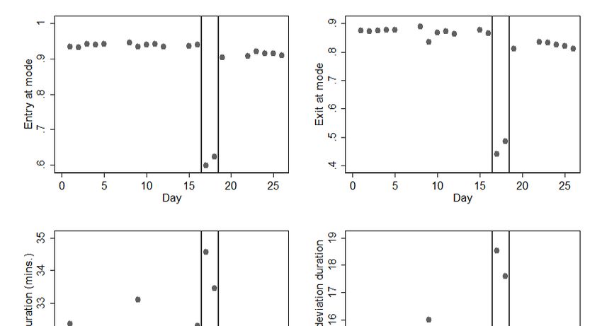
Finally, Figure 4 shows the evolution of some key variables of interest for all weekdays
in our sample period. The top-left panel shows the fraction of commuters (identi…ed as
described in Section 4) who enter at their modal station, while the top-right panel shows
the same at the exit-margin. The two strike days can be found in between the vertical
lines. As one can see from the two panels, far less commuters were able to use their
modal station during the strike –which implies that a substantial number of individuals
was forced to explore alternative routes. Moreover, the post-strike data also suggest that
the strike brought about some lasting changes in behavior, as the fraction of commuters
that makes use of their modal station seems to drop after the strike.14
14
Establishing this more formally is the objective of the remainder of this paper.
10The lower two panels of Figure 4 provide information on journey times: as the bottom-
left panel shows, the duration of the average journey on London’s public transport system
went up during the strike (by about 6%), while the bottom-right panel shows that this
increase in average duration was also accompanied by an increase in dispersion.
[Insert Figure 4 about here]
6 Method
Our dataset lends itself perfectly for a di¤erence-in-di¤erences exercise, which is the ap-
proach that we will take in this paper. After all, we are ultimately interested in the
question whether individuals who were "treated" (i.e.: forced to experiment) during the
strike, went on to behave any di¤erently from their non-treated peers in the post-strike
period. Consequently, we will typically estimate regression equations that are of the
following form:
dmode
it = i+ dpost
t + dpost
t dtreat
i + it (1)
Here, dmode
it is a dummy-variable that takes the value 1 if individual i makes his "modal
journey" (i.e.: travels from his modal station of entry to his modal station of exit) on date
t, dpost
t is a dummy-variable that takes the value 1 in the post-strike period, while dtreat
i is
a dummy-variable that takes the value 1 if individual i was part of the treatment group.
Data from the two strike days is not used for estimation-purposes. We estimate equation
(1) via OLS (but probit yields very similar results, see Section 7) and calculate robust
standard errors. We also include individual …xed-e¤ects as captured by i in equation (1).
The reason is threefold. Firstly, …xed e¤ects control for unobserved demographic factors
(such as age) that may a¤ect an individual’s inclination to experiment. In a similar vein,
they are able to control for area-characteristics (since one area may be more amenable
to experimentation than another). Thirdly, …xed e¤ects also correct for the fact that
di¤erent individuals use their modal station with di¤erent intensity.
Finally, it in equation (1) is the error-term, measures time e¤ects, while captures
the treatment e¤ect. However, as we will clarify in the remainder of this section, iden-
tifying the treatment group from our dataset is non-trivial. Consequently, we will show
results for three di¤erent de…nitions of treated commuters –where all measures have their
speci…c advantages and disadvantages.
Our …rst measure of treatment simply de…nes treated individuals as all those who devi-
ated from their pre-strike modal journey during the strike. This would include individuals
11who were forced to explore a new route due to closure of an entry, exit, or connecting sta-
tion, but will also encompass those who deviated from their pre-strike mode for non-strike
related reasons.
Our second measure of treatment takes a more direct approach: in this exercise, we
take individuals to be treated if their pre-strike modal station (either entry and/or exit)
was to be closed down during the strike. After all, we can be reasonably sure that these
individuals were not able to travel to or from their modal station during the strike –as a
result of which they were de…nitely forced to explore alternatives. This measure however
su¤ers from the fact that it is likely to pool a signi…cant number treated individuals with
the non-treated group. The reason is that many individuals in our dataset travel from
station A to station B via at least one connecting station C. Closure of the latter would
force this individual to explore alternatives, but unfortunately we don’t observe connecting
stations in our data (only stations of entry and exit). Consequently, our second measure
of treatment is likely to lead to type II errors and underestimate the true e¤ect.
Our third measure of treatment is somewhat di¤erent and based upon travel time: here
we take individuals to be treated if their travel times during strike days were su¢ ciently
di¤erent (i.e.: longer or shorter) from their travel times during the pre-strike period. This
method identi…es those commuters who had a very unusual experience during the strike as
measured by time. It does not rely upon our de…nition of closed stations (as pointed out
in Section 3, some stations were only partially closed), while it also side-steps our concept
of "deviations from the modal commute". This measure of treatment is however prone
to errors of both the …rst and the second kind (i.e.: there will be both "false positives"
and "false negatives"). After all: if an individual had a di¤erent journey time on strike
days, that does not necessarily imply that he was actually exploring an alternative route.
It could simply be the case that his modal route took much longer due to congestion
on the network, or due to a reduction in the number of trains running. Similarly, it is
also possible that a commuter explored a di¤erent route, but that this did not lead to a
markedly di¤erent travel time.
7 Findings
In this section we will present our main …ndings. Section 7.1 describes outcomes of the
most fundamental regressions that we ran, Section 7.2 studies the robustness of these
results, Section 7.3 analyzes the e¤ects on travel time, after which Section 7.4 tries to
understand what drives our core …ndings.
127.1 Core results
As set out in Section 6, we rely upon di¤erence-in-di¤erences estimations to ask whether
treated commuters were more likely to deviate from their pre-strike modal journey in the
post-strike period, relative to their non-treated peers. The answer to this question can
be found by looking at the sign of our estimate of the treatment e¤ect in regression
equation (1).
Our estimates, reported in Table 1, strongly suggest that those who were forced to
explore alternatives during the strike, were less likely to return to their pre-strike modal
commute after the restriction was lifted. This result is robust to di¤erent estimation
strategies (as we will document below), while it arises no matter how we de…ne the
treatment group: in Column 1, the treatment group consists of all individuals who deviated
from their modal morning commute during the strike. Column 2 includes commuters in
the treatment group if their pre-strike modal commute started or ended at a station
which was closed during the strike. In the last three columns of Table 1, individuals are
considered to be part of the treatment group if they experienced a substantially longer or
shorter journey time during the strike. The "factor" indicated in the top-row considers
di¤erent de…nitions of "substantially": a factor 1.2 for example implies that an individual
was included in the treatment group if his average morning commute during the strike
was at least 20% longer or shorter than his pre-strike average.
In all three exercises, the interaction coe¢ cient (measuring the di¤erence-in-di¤erences)
is consistently estimated to be signi…cantly negative. This implies that individuals who
were part of the treatment group (i.e.: those who were forced to explore alternative routes
during the strike), were less likely to return to their pre-strike modal commute in the post-
strike period.15 By a revealed preference-type argument, this suggests that a signi…cant
fraction of commuters had failed to …nd their optimal journey before the strike. After
all: post-strike, all routes were available again (including the pre-strike modal one) so a
failure to pick the latter option suggests that the commuter has found a better alternative
during the disruption.
Our results are unlikely to be driven by a change in habits. Not only do they typically
take much longer to be established (Wood and Neal, 2009), but the observed behavior
of commuters is also inconsistent with this hypothesis: after the strike, many of them
continue to explore alternative routes (leading to a prolonged "experimental phase") after
which they eventually settle on a new modal choice.16
15
In the speci…cation where we identify the treatment group via the time factor, this e¤ect is consistently
stronger for those travelers who experienced a shorter commute during the strike, which is intuitive.
16
To give a random example: one commuter in our dataset consistently traveled from Sydenham to
13Looking at the magnitudes of estimates across the various tables is informative as well.
Doing so shows that our estimate of the treatment e¤ect is signi…cantly larger in Column
1, while that of (the coe¢ cient on the post-strike dummy dpost t ) is signi…cantly smaller.
From a theoretical point of view, there is reason to be suspicious of a large negative es-
timate for (as visible in Columns 2-5): the tube-network itself did not change during
our short sample period (nor does our sample include any other noteworthy events), so
there is no reason why non-treated commuters should suddenly start to display di¤erent
behavior post-strike. To us, the large negative estimates for the coe¢ cient on dpost
t there-
fore suggest that our last two treatment-de…nitions err by including treated individuals in
the non-treated group. As anticipated in Section 6, it is to be expected that our second
measure of treatment is particularly prone to this statistical error of the second kind –and
indeed, the absolute value of the estimate of is lowest in this speci…cation, while that
of is highest. In Column 1 on the other hand, the estimate of is close to zero (which
makes sense from a theoretical point of view), as a result of which this table contains our
preferred estimates for the treatment e¤ect .
Table 1: OLS-DiD results.17
(1: not on mode) (2: mode on strike) (3: factor 1.2) (4: factor 1.5) (5: factor 2)
dmode
it dmode
it dmode
it dmode
it dmode
it
dpost
t -0.0108*** -0.0466*** -0.0402*** -0.0464*** -0.0504***
(0.00186) (0.00185) (0.00175) (0.00140) (0.00128)
dpost
t dtreat
i -0.0569*** -0.00860*** -0.0205*** -0.0201*** -0.0113**
(0.00242) (0.00248) (0.00245) (0.00293) (0.00451)
obs18 312,156 312,156 312,156 312,156 312,156
To understand where the results of Table 1 are coming from, one can also increase
the level of detail and estimate a speci…cation that distinguishes between entry and exit
Canary Wharf in the pre-strike period. During the strike, (s)he experiments with entering at Elverson
Road (using the DLR to travel to Canary Wharf). In the post-strike period, (s)he …rst alternates between
both options (seemingly comparing them) after which (s)he settles for the newly-found DLR-based route.
There are also more determined examples: another commuter consistently travels from Richmond to
St. James on every morning before the strike. Both stations however closed down during the strike,
in response to which (s)he switched to traveling from North Sheen to Waterloo on the …rst strike day.
Subsequently, (s)he sticks with this new alternative (which has a shorter duration and a lower variance)
for the remainder of our sample period.
17
In this table, as well as in all tables that are to follow, * denotes signi…cance at the 10% level, **
implies signi…cance at the 5% level, while *** indicates signi…cance at the 1% level.
18
The number of treated commuters is: 243,254 for Column (1), 188,080 for (2), 185,081 for (3), 83,380
for (4) and 28,732 for (5).
14entry_mode exit_mode
(so the LHS-variable in that regression is either dit or dit ). Results of this
exercise, recorded in Table 2, indicate that the treatment e¤ect tends to be bigger at the
exit-end. This is intuitive since the exit-end of the morning commute tends to lie in the
city center (recall Figure 2) where station-density, and hence substitutability, is higher.
Also note that Table 2 contains only two estimates (in italics) that are not signi…cant
at any regular level of signi…cance (whereas all other estimates are signi…cant at the 1%
level). However, they show up at exactly those places where this is plausible, namely
when we look at what closure of a modal exit station does to the choice of station of entry
(and vice versa).
Table 2: Estimates of when distinguishing between entry and exit margin.19
Treatment de…nition (1) (2)
entry_mode exit_mode
dit dit
not on mode -0.0267*** -0.0470***
(0.00164) (0.00224)
either on strike -0.00480*** -0.00480***
(0.00170) (0.00170)
entry on strike -0.00697*** 0.000569
(0.00190) (0.00247)
exit on strike -0.00146 -0.00748***
(0.00173) (0.00230)
time factor(1.2) -0.0141*** -0.0154***
(0.00168) (0.00227)
time factor(1.5) -0.0111*** -0.0175***
(0.00207) (0.00270)
time factor(2) -0.00766*** -0.0113***
(0.00329) (0.00411)
obs 312,156 312,156
The coe¢ cients in Tables 1 and 2 are however not straightforward in their interpre-
tation due to the probabilistic nature of our exercise (driven by the fact that commuters
in our pre-strike sample only make their modal journey for about 84% of the time on
average): an estimate for of -0.03, for example implies that treated individuals will
19
Note that this table is based upon 14 regressions of the same form as equation (1). For space-
constraints, we only report our estimates of . In Column 1 we report results when the dependent
variable is a dummy for entry at mode, while Column 2 reports estimates for a dummy for exit at mode.
15make their pre-strike modal commute with a probability that is 3 percentage points lower
compared to their non-treated peers. This does however not imply that 3% is also the
fraction of switchers in our sample.
Table 3, on the other hand, does produce information on the fraction of switchers –as
such a number is arguably easier to interpret for our purposes. This table is constructed
by …rst identifying those commuters who made the exact same morning commute (as
far as stations of entry and exit are concerned) during all 10 working days of our pre-
strike sample. Hence, all these individuals (whom we refer to as "pre-strike habituals")
are selected so that they make their modal commute with probability 1 in the pre-strike
period. We subsequently ask: how many percentage points higher is the fraction of "post-
strike switchers"20 in the treatment group relative to the fraction of switchers among
non-treated commuters?21
Table 3: Fraction of switchers among pre-strike habituals.
Treatment de…nition
not on mode 5.42%
mode on strike 2.64%
time factor(1.2) 1.24%
time factor(1.5) 1.86%
time factor(2) 2.81%
obs 6,946
As can be seen from the table, our data suggest that (depending on whom we consider
to be treated) the fraction of post-strike switchers is 1.2 to 5.4 percentage points higher
in the treatment group. Since results for our last two measures of treatment are again
likely to be biased by type II errors, we believe that the true number lies closer to 5.4
percentage points (the number we obtain when de…ning the treatment group as those
who deviated from their modal journey during the strike). This is a strong result as the
20
Here, "switchers" are de…ned as those individuals who made a di¤erent commute than their pre-strike
modal journey on the last working day of our sample (Friday February 14). This exercise therefore assumes
that the "experimentation phase", triggered by the strike-induced forced episode of experimentation, was
over by this time (also recall footnote 16). Requiring them to deviate for more than one day, yields very
similar results.
21
Here, it is absolutely essential to look at results relative to a non-treated control group since this
exercise is obviously prone to "regression to the mean": given that the habituals were using their modal
station with probability 1 in the pre-strike period, they can only make (weakly) less use of it post-strike.
The control group of non-treated commuters allows us to correct for mean reversion.
16individuals underlying this exercise all seemed to be stuck in a very regular habit before
the strike (as they were selected exactly because they were making the same commute on
every single morning in the pre-strike sample). The selection method could furthermore
imply that these commuters have only few viable alternatives available, which also biases
the results against switching. Moreover, exploring a new route during a tube strike is
typically not a pleasant experience (due to the associated chaos and crowdedness, while
there were also fewer trains running during the February 2014-strike – causing further
delays). Consequently, it is likely that results would be even larger after considering
voluntary experimentation under tranquil conditions. In line with our earlier …ndings,
this again provides evidence that a substantial proportion of commuters had failed to …nd
their maximum before the tube strike of February 2014.22
7.2 Robustness
We have found our results to be very robust to alternative regression speci…cations. This
can for example be seen from Table 4.
Table 4: Estimates of across speci…cations.23
Treatment de…nition (1: probit) (2: BDM) (3: SL)
dmode
it dmode
it dmode
it
not on mode -0.358*** -0.0569*** -0.0414***
(0.0144) (0.00311) (0.00540)
either on strike -0.0341*** -0.00860*** -0.0208***
(0.0118) (0.00333) (0.00608)
time factor(1.2) -0.107*** -0.0205*** -0.0116**
(0.0119) (0.00331) (0.00568)
time factor(1.5) -0.0977*** -0.0201*** -0.0223***
(0.0135) (0.00406) (0.00664)
time factor(2) -0.0572*** -0.0113* -0.0337***
(0.0208) (0.00615) (0.0105)
obs 312,156 34,684 47,052
22
Do note that we are not claiming that these commuters have found their global maximum post-strike:
all we are saying is that they have found something better than their pre-strike mode, but it is very well
possible that further improvements are still possible.
23
As with Table 2, this table is based upon 15 underlying regressions of the same form as equation (1).
For space-constraints, we only report our estimates of .
17The …rst column of this table shows our results for when estimated with probit
(conveniently, probit-coe¢ cients and marginal e¤ects coincide in this case as there are
no continuous covariates). Estimates obtained in this way continue to be signi…cantly
negative, but suggest an even larger treatment e¤ect.
A well-known criticism of OLS-DiD panel data regressions, is that autocorrelation in
the observations arti…cially decreases standard errors (Bertrand, Du‡o and Mullainathan,
2004; henceforth "BDM"). In column 2, we therefore report results generated by BDM’s
most conservative robustness check –namely the one where the data are collapsed to two
observations for each individual: one observation pre-strike and one post-strike (and we
collapse our LHS variable by computing the mean number of modal journeys before and
after the strike). As these columns show, coe¢ cients remain numerically identical in this
exercise and still are highly signi…cant.
Finally, column 3 shows our baseline estimates of when we restrict our sample to
those individuals who enter and exit on the same line ("SL"). As set out before, identifying
the treatment group is somewhat challenging in the full sample as many individuals
make use of connecting stations during their commute. Closure of a connecting station
implies that such an individual was treated during the strike (even if his entry and exit
station remained open), but unfortunately we do not observe data on connections. This
concern plays no role when we limit ourselves to those commuters who enter and exit
on the same line (as they are unlikely to travel via a connecting station). Due to the
"same line"-restriction we are left with fewer observations, but our main result continues
to emerge – albeit somewhat less signi…cantly (which is no surprise given the smaller
sample size) and typically smaller in magnitude. The latter is to be expected since the
scope for experimentation is substantially smaller for commuters who use only one line
(commuters who use multiple lines and connections have more dimensions along which
they can deviate).
7.3 E¤ects on travel time
A follow-up question to ask at this stage is: what was the e¤ect of the strike on commuting
times? Unfortunately, we do not observe the duration of the entire commute (since com-
muters are not on our radar before they check-in to/after they check-out of TfL-services),
but we can calculate the amount of time they spent on London’s public transport network.
After calculating these durations, we estimate the following –now familiar –regression:
ln(durationit ) = i + dpost
t + dpost
t dtreat
i + it
18Note that our dependent variable is the natural logarithm of duration (so that coef-
…cients can conveniently be interpreted as percentages). Once more, our main interest
lies in the estimate of . Estimation results are shown in Table 5 below (again for our
…ve di¤erent characterizations of the treatment group). As can be seen from the table,
our estimate of is consistently negative which suggests that commuters who were part
of the treatment group were able to cut their "time spent on public transport" by more
than their non-treated peers. On average, the treatment group seems to be able to cut
their journey time by about 1% more. Given that the average journey in our sample
lasts approximately 32 minutes, this amounts to a time-gain of about 20 seconds on a
one-way commute. Note that the 20 seconds-…gure is an average taken over those treated
commuters who found a better route post-strike, and those who did not (and stayed with
their pre-strike mode as a result).
As pointed out before, this is only part of the complete story since the new route
may also be preferred along other characteristics that remain unobserved to us (like train
crowdedness or the nature of the follow-up journey). Consequently, we see the utility-
equivalent of this time-gain as a lower-bound on the true welfare-gains.
Table 5: OLS-DiD results for travel time
(1: not on mode) (2: mode on strike) (3: factor 1.2) (4: factor 1.5) (5: factor 2)
ln(durationit ) ln(durationit ) ln(durationit ) ln(durationit ) ln(durationit )
dpost
t 0.00711*** 0.00113 0.00125 0.000670 -0.000698
(0.00164) (0.00158) (0.00132) (0.00108) (0.00103)
dpost
t dtreat
i -0.0124*** -0.00518** -0.00548*** -0.00977*** -0.0121***
(0.00206) (0.00204) (0.00198) (0.00261) (0.00430)
obs 312,103 312,103 312,103 312,103 312,103
7.4 Mechanism
Given that the previous sections have established that treated commuters were more likely
to switch (and cut travel time) in the post-strike period than their non-treated peers,
a logical follow-up question is: why? In the remainder of this section, we will provide
evidence which suggests that this is due to the existence of informational imperfections.
To provide evidence for the importance of informational imperfections, we use in-
formation on two characteristics of the London underground system that are not easily
observed by commuters, namely map distortion (Section 7.4.1) and line speed (Section
7.4.2).
197.4.1 Map distortion
As noted before, an important source of imperfect information is the fact that the London
tube map provides a distorted picture of reality. For the exercise in this subsection, we
quantify these distortions in the following way. For each station on the map (s) we list
those stations that lie within a 2 kilometer radius (which is about a 20 minute walk) from
s.24 We subsequently correlate the true distance between these stations, with the distance
on the tube map (which we have digitized). Subtracting the resulting correlation from 1,
gives our measure for distortion.
The outcome of this exercise shows that map distortions are not constant across Lon-
don: some people live in areas where the tube map is more distorted than others (the
general rule being that distortion increases with distance to central London).
Thanks to this spatial variation, we are able to ask: do commuters who live in areas
that are more distorted on the London tube map, have greater di¢ culty in …nding their
preferred route? And do they learn more from the strike as a result? To answer this
question, we estimated the following di¤erence-in-di¤erence-in-di¤erences regression:
j_mode
dit = i+ dpost
t + dpost
t dtreat
i + dpost
t distji + dpost
t dtreat
i distji + it ; (2)
where "distji " is our measure of map distortion around individual i’s modal station of
entry or exit (with j2 fentry,exitg). Note that this exercise again explicitly distinguishes
between the station of entry and exit, since map distortions are likely to be di¤erent at
both ends. Tables 6-8 report our results.
In this regression, a negative estimate for would suggest that treated commuters who
live in (or travel to) more distorted areas, are less likely to return to their pre-strike modal
journey in the post-strike period. This would provide evidence in favor of the hypothesis
that commuters who live in more distorted areas, have greater di¢ culty in …nding their
optimal commute. And as can be seen from Tables 6-8, this indeed seems to be the case:
our estimate of tends to be signi…cantly negative across speci…cations, thereby pointing
towards the importance of informational imperfections in explaining our …ndings.
24
Very similar results are obtained if we use a radius of 5 kilometer.
20Table 6: OLS-DiD results when treatment group is identi…ed as individuals deviating from
pre-strike mode during strike.
(1) (2)
entry_mode exit_mode
dit dit
dpost
t -0.00440 -0.00317
(0.00364) (0.00511)
dpost
t distji 0.00141 -0.0435
(0.0250) (0.0338)
dpost
t dtreat
i -0.0152*** -0.0407***
(0.00478) (0.00661)
dpost
t dtreat
i distji -0.0675** -0.0263
(0.0327) (0.0438)
obs 267,588 267,588
Table 7: OLS-DiD results when treatment group is identi…ed as individuals traveling to or
from a¤ected stations pre-strike.
(1: entry on strike) (2: exit on strike) (3: either) (4: either)
entry_mode exit_mode entry_mode exit_mode
dit dit dit dit
dpost
t -0.0196*** -0.0186*** -0.0210*** -0.0350***
(0.00272) (0.00612) (0.00359) (0.00510)
dpost
t distji 0.00306 -0.115*** 0.0103 -0.00363
(0.0207) (0.0431) (0.0254) (0.0350)
dpost
t dtreat
i 0.0110** 0.00335 0.00927* 0.00278
(0.00482) (0.00838) (0.00494) (0.00677)
dpost
t dtreat
i distji -0.160*** -0.142** -0.0996*** -0.0971**
(0.0376) (0.0612) (0.0340) (0.0455)
obs 226,404 184,482 267,588 267,588
21Table 8: OLS-DiD results when treatment group is identi…ed by travel time.
(1) (2) (3) (4) (5) (6)
entry_mode exit_mode entry_mode exit_mode entry_mode exit_mode
dit dit dit dit dit dit
dpost
t -0.0101*** -0.0230*** -0.0158*** -0.0265*** -0.0177*** -0.0317***
(0.00342) (0.00479) (0.00278) (0.00382) (0.00256) (0.00351)
dpost
t distji -0.0428* -0.0782** -0.0323* -0.0820*** -0.0316* -0.0712***
(0.0235) (0.0320) (0.0189) (0.0254) (0.0174) (0.0233)
dpost
t dtreat
i -0.0103** -0.0183*** 0.000678 -0.0257*** 0.0224** -0.0124
(0.00490) (0.00668) (0.00597) (0.00793) (0.00942) (0.0188)
dpost
t dtreat
i distji -0.0111 0.0207 -0.0712* 0.0540 -0.208*** 0.0109
(0.0333) (0.0444) (0.0402) (0.0525) (0.0633) (0.0784)
obs 267,588 267,588 267,588 267,588 267,588 267,588
factor 1.2 1.2 1.5 1.5 2 2
7.4.2 Line speed
Even if the London underground network were to adopt an undistorted tube map, this
still would not solve all informational problems. The reason is that many characteristics of
various lines (such as crowdedness, nature of the follow-up journey to work, etc.) remain
unknown until that line is actually tried. One such characteristic that is easily quanti…ed,
is line speed. As shown in Table 9, speed di¤ers considerably across lines.25 Consequently,
two journeys that look equally far on an undistorted map, are still not equivalent if they
are made in trains that travel at di¤erent speeds.
Table 10 therefore reports results that were obtained after estimating the following
di¤erence-in-di¤erence-in-di¤erences regression:
dmode
it = i+ dpost
t + dpost
t dtreat
i + dpost
t speedi + dpost
t dtreat
i speedi + it (3)
Since speed varies across lines, we now limit ourselves to the sample of commuters
who stay on the same underground line for their entire commute (the same sample that
was used in Column 3 of Table 4). Consequently, our speed-variable becomes individual i-
speci…c. The "same line"-restriction reduces sample size, as a result of which our estimates
become less signi…cant (like in Table 4).
25
This table draws upon own calculations (based upon TfL-information) and contains the average speed
attained by the various trains in between stations. Consequently, our measure is not distorted by the
density of stations on a particular line, which is a characteristic that is easily observed from the tube
map.
22You can also read