The color out of space: learning self-supervised representations for Earth Observation imagery - arXiv
←
→
Page content transcription
If your browser does not render page correctly, please read the page content below
The color out of space: learning self-supervised
                                                representations for Earth Observation imagery
                                                        Stefano Vincenzi∗ , Angelo Porrello∗ , Pietro Buzzega∗ , Marco Cipriano∗ , Pietro Fronte‡ ,
                                                                Roberto Cuccu‡ , Carla Ippoliti† , Annamaria Conte† , Simone Calderara∗
                                                                          ∗ AImageLab,    University of Modena and Reggio Emilia, Modena, Italy
                                                           † Istituto   Zooprofilattico Sperimentale dell’Abruzzo e del Molise ‘G.Caporale’, Teramo, Italy
                                                                                      ‡ Progressive Systems Srl, Frascati – Rome, Italy

                                            Abstract—The recent growth in the number of satellite images          step is carried out on a target task (e.g. land cover classi-
                                         fosters the development of effective deep-learning techniques for        fication). This way, one can achieve acceptable results even
                                         Remote Sensing (RS). However, their full potential is untapped           in the presence of few labeled examples, as the second step
                                         due to the lack of large annotated datasets. Such a problem
                                         is usually countered by fine-tuning a feature extractor that             just adapts a set of general-purpose features to the new task.
arXiv:2006.12119v1 [cs.CV] 22 Jun 2020

                                         is previously trained on the ImageNet dataset. Unfortunately,            However, this approach is limited only to the tasks involving
                                         the domain of natural images differs from the RS one, which              RGB images as input. Satellite imagery represents a domain
                                         hinders the final performance. In this work, we propose to learn         that is quite different from the RGB one, thus making the
                                         meaningful representations from satellite imagery, leveraging            ImageNet pre-training only partially suitable.
                                         its high-dimensionality spectral bands to reconstruct the visible
                                         colors. We conduct experiments on land cover classification                 These considerations reveal the need for novel approaches
                                         (BigEarthNet) and West Nile Virus detection, showing that                that are tailored for satellite imagery. To build transferable
                                         colorization is a solid pretext task for training a feature extractor.   representations, two kinds of approaches arise from the lit-
                                         Furthermore, we qualitatively observe that guesses based on              erature: annotation-based methods and self-supervised ones.
                                         natural images and colorization rely on different parts of the           The authors of [11] fulfill the principle of the first branch
                                         input. This paves the way to an ensemble model that eventually
                                         outperforms both the above-mentioned techniques.                         by investigating in-domain representation learning. They shift
                                                                                                                  the pre-training stage from ImageNet to a labeled dataset
                                                               I. I NTRODUCTION                                   specific for remote sensing. As an example, one could leverage
                                            Over the last decades, Remote Sensing has become an                   BigEarthNet [12], which has been recently released for land-
                                         enabling factor for a broad spectrum of applications such                cover classification. On the other hand, Tile2Vec [13] extracts
                                         as disaster prevention [1], wildfire detection [2], vector-borne         informative features in a self-supervised fashion. The authors
                                         disease [3], and climate change [4]. These applications benefit          rely on the assumption that spatially close tiles share simi-
                                         from a higher number of satellite imagery captured at unprece-           lar information: therefore, their corresponding representations
                                         dented rhythms [5], thus making every aspect of the Earth’s              should be placed closer than tiles that are far apart. In doing so,
                                         surface constantly monitored. Machine learning and Computer              one does not need labeled data for extracting representations,
                                         Vision provide valid tools to exploit these data in an efficient         but lacks robustness when close tiles are not similar.
                                         way. Indeed, a synergy between Earth Observation and Deep                   Similarly to [13], we propose a novel representation learn-
                                         Learning techniques led to promising results, as highlighted by          ing procedure for satellite imagery, which devises a self-
                                         recent advances in land use and land cover classification [6],           supervised algorithm. In more detail, we require the network to
                                         image fusion [7], and semantic segmentation [8].                         recover the RGB information by means of other spectral bands
                                            Despite the amount of raw information being significant,              solely. For the rest of the article, we adopt the term “spectral
                                         the exploitation of these data still raises an open problem.             bands” for indicating the subset of the bands not including
                                         Indeed, the prevailing learning paradigm – the supervised one            the RGB. Our approach closely relates to colorization, which
                                         – frames the presence of labeled data as a crucial factor.               turns out to encourage robust and high-level feature represen-
                                         However, acquiring a huge amount of ground truth data is                 tations [14], [15]. We feel this pretext task being particularly
                                         expensive and requires expert staff, equipment, and in-field             useful for satellite imagery, as the connection between colors
                                         measurements. This often restrains the development of many               and semantics appears strong: for instance, sea waters feature
                                         downstream tasks that are important for paving the way to the            the blue color, vegetation regions the green one or arable lands
                                         above-mentioned applications.                                            prefer warm tones. We inject such a prior knowledge through
                                            To mitigate such a problem, a common solution [9] exploits            an encoder-decoder architecture that – differently from concur-
                                         models that are pre-trained on the ImageNet [10] dataset. In             rent works – exploits spectral bands (e.g. short-wave infrared,
                                         detail, the learning phase is conducted as follows: firstly, a           near-infrared, etc.) instead of grayscale information to infer
                                         deep network is trained on ImageNet until it reaches good                color channels. Once the model has reached good capabilities
                                         performance on image categorization; secondly, a fine-tuning             on tile colorization, we use its encoder as a feature extractor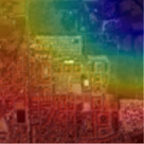
for the later step, namely fine-tuning on a remote sensing task.       translation, and rotation), which increases both the diversity
We found that the representations learnt by colorization leads         and volume of training data.
to remarkable results and semantically diverge from the ones
computed on top of RGB channels. Taking advantage of these             B. Unsupervised Representations Learning
findings, we set up an ensemble model, which averages the                 Unsupervised and self-supervised methods were introduced
predictions from two distinct branches at inference time (the          to learn general visual features from unlabeled data [22].
one fed with spectral bands, the other with RGB information).          These approaches often rely on pretext tasks, which attempt
We show that ensembling features this way leads to better              to compensate for the lack of labels through an artificial
results. To the best of our knowledge, our work is the first           supervision signal. In so doing, the learned representations
investigating colorization as a guide towards suitable features        hopefully embody meaningful information that is beneficial to
for remote sensing applications.                                       downstream tasks.
   To show the effectiveness of our proposal, we assess it             Reconstructions-based methods. Under this perspective, gen-
in two different settings. Firstly, we conduct experiments on          erative models can be considered as self-supervised methods,
land-cover classification, comparing our solution with two             where the reconstruction of the input acts as a pretext task.
baselines, namely training from scratch and fine-tuning the            Denoising Autoencoders [23] contribute to this line of re-
ImageNet pre-training. We show that colorization is particu-           search: here, the learner has to recover the original input from
larly effective when few annotations are available for the target      a corrupted version. The idea is that good representations are
tasks. This makes our proposal viable for scenarios where              those capturing stable patterns, which should be recovered
gathering many labeled data is not practicable. To demonstrate         even in the presence of a partial or noisy observation. In
such a claim, we additionally conduct experiments on the               remote sensing, autoencoders are often applied [16], [24], [25]
“West Nile Virus” cases collected in the frame of the Surveil-         to reduce the dimensionality of the feature space. This yields
lance plan put in place by the Ministry of Health, with the aim        the twofold advantage of decreasing the correlation lying in
of predicting presence/absence across the Italian territory.           spectral bands and reducing the overall computational effort.
                                                                       Classification-based methods. [26] frames the pretext task
                     II. R ELATED W ORKS                               as a classification problem, where the learner guesses which
                                                                       rotation (0, 90, 180 and 270) has been applied to its input.
A. Land cover - Land use classification
                                                                       The authors observe that recognizing the input transformation
   Recently, the categorization of land-covers has attracted           behaves as a proxy for object recognition: the higher the
wide interest, as it allows for the collection of statistics, activ-   accuracy on the upstream task, the higher the accuracy on
ities planning, and climate changes monitoring. To address             the downstream one. Considering two random patches from a
these challenges, the authors of [16] exploit Convolutional            given image, [27] asks the network to infer the relative position
Neural Networks (CNN) to extract representations encoding              between those. This encourages the learner to recognize the
both spectral and spatial information. To speed up the learning        parts that make up the object as well as their relations. Simi-
process, they advocate for a prior dimensionality reduction            larly, [28] presents a jigsaw puzzle to the network, which has
step across the spectra, as they observe a high correlation in         to place the shuffled patches back to their original locations.
this dimension. Among works focusing on how to exploit spec-           Colorization-based methods. Given a grey-scale image as
tral bands, [17] devises Recurrent Neural Networks (RNNs) to           input, colorization is the process of predicting realistic colors
handle the redundancy underlying adjacent spectral channels.           as output. A qualitative analysis conducted in [29] shows that
Similarly, [18] proposes a 3D-CNN framework, which can                 colorization-driven representations capture semantic informa-
naturally joint spatial and spectral information in an end-to-         tion, grouping together high-level objects that display low-
end fashion without requiring any pre-processing step.                 level variations (e.g. color or pose). [30] concerns the ambi-
   While these approaches concern the design of the feature            guity and ill-posedness of colorization, arguing that several
extractor, our work is primarily engaged in the scenarios in           solutions may be assessed for a given grey-scale image. On
which few labeled examples are available. In these contexts,           this basis, the authors exploit Conditional Variational Autoen-
fine-tuning pre-trained models often mitigate the lack of a            coder (CVAE) to produce diverse colorizations, thus naturally
large annotated dataset, yielding great performance in some            complying with the multi-modal nature of the problem. In-
cases [19], [20]. Intuitively, the representations learned from        stead, [31] focuses on the design of the inference pipeline and
ImageNet (1 million images belonging to 1000 classes) en-              proposes a two-stage procedure: i) a pixel-wise descriptor is
code a prior knowledge on natural images, thus facilitating            built by VGG-16 feature maps taken at different resolutions;
the transfer to different domains. Instead, [11] proposes in-          ii) the descriptors are then fed into a fully connected layer,
domain fine-tuning, where the pre-training stage performs              which outputs hue and chroma distributions. Split-Brain Au-
on a remote sensing dataset. The authors found in-domain               toencoders [15] relies on a network composed of two disjoint
representations to be especially effective with limited data           modules, each of which predicts a subset of color channels
(1000 training examples), surpassing the performance yielded           from another. The authors argue that this schema induces
by the ImageNet initialization. As a final remark, one could           transferable representations, the latter taking into account all
reduce overfitting through data augmentation [21] (i.e. flip,          input dimensions (instead of gray-scale solely).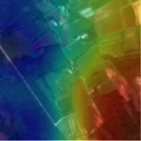
III. M ODEL                                 Colorization Loss. Recent works [15], [29], [32] investigate
                                                                      various loss functions, questioning their contributions to col-
Overview. Our main goal consists in finding a good initial-
                                                                      orization results (intended as performance on either the target
ization for the classifier, in such a way that it can later capture
                                                                      task or the pretext one). Despite a regression objective (e.g. the
meaningful and robust patters even in presence of few labeled
                                                                      mean squared error) being a valid baseline, these works show
data. To this purpose, we devise a two-stage procedure tailored
                                                                      that treating the problem as a multinomial classification leads
for satellite imagery tasks, which prepends a colorization step
                                                                      to better results. However, the overall training time increases
(Sec. III-A) to a fine-tuning one (Sec. III-B).
                                                                      considerably because of the additional information taken into
   As depicted in Fig. 1 (a), our proposal leverages an encoder-
                                                                      account. In our case, this would add up to the burdensome
decoder architecture for feature learning. In doing so, we
                                                                      computations required by hyperspectral images, thus resulting
do not require the model to reconstruct its input: differently,
                                                                      even more expensive. For this reason, we limit our experiments
we set up an asymmetry between input (spectral bands) and
                                                                      to the mean absolute error L1 (·, ·), as follows:
output (color channels). This way, we expect the encoder to
capture meaningful information about soil and environmental                               X (a)           (a)       (b)     (b)
                                                                          L1 (X,
                                                                               b X) = λ        bh,w − xh,w + x
                                                                                               x                  bh,w − xh,w , (1)
characteristics. Afterward, we exploit the encoder and its rep-
                                                                                          h,w
resentation capabilities to tackle a downstream task (e.g. land
cover classification, see Fig. 1 (b)). Eventually, an ensemble        where X represents the a∗b ground truth colorization and λ =
model (see Sec. III-C for additional details) further refines         100 is a weighting term that prevents numerical instabilities.
the final prediction combining the outputs from the two input
modalities (RGB and spectral bands).                                  B. Fine-tuning

A. Colorization                                                          Once the encoder-decoder has been trained, we turn our
                                                                      attention to the downstream task and exploit the encoder F(·)
   In formal terms, the encoder network F takes S ∈                   as a pre-trained feature extractor. To achieve this, we need a
RH×W ×C as input, where C equals the number of spectral               single amendment to the network: a final linear transformation
bands available to the model and H and W the input resolution         that maps bottleneck features H = F(S) to the classification
(height and width respectively). The decoder network produces         output space y b = WT H + b.
a tensor X b ∈ RH×W ×2 , which yields the pixel-wise predic-
                                                                      Classification Loss We make use of two different losses
tions in terms of a and b coordinates in the CIE Lab color
                                                                      in our experiments: when dealing with a multi-label task
space. On this latter point, a naive strategy would simply define
                                                                      as the land cover classification one (i.e. each example can
the expected output in terms of RGB: nevertheless, as pointed
                                                                      be categorized into multiple classes), the objective function
out in [31], modeling colors as RGB values may not yield an
                                                                      resembles a binary cross-entropy term averaged over C classes:
effective training signal. Differently, we adhere to the guideline
described in [32] and frame the problem in the CIE Lab space.                       1 X
Here, a color is defined with a lightness component L and a∗b         L(b
                                                                        y, y) = −                 yi ) + (1 − yi ) log (1 − σ (b
                                                                                        yi log σ (b                            yi )) ,
                                                                                    C i
values carrying the chromatic content. The effectiveness of this
space comes from the fact that colors are encoded accordingly         where y indicates the ground-truth multi-hot encoding vector
to human perception: namely, the distance between two points          and σ the sigmoid function. Differently, we use the binary
reflects the amount of visually perceived change between the          cross-entropy loss to treat the West Nile Disease case study.
corresponding colors.
Encoder. We opt for ResNet18 [33] as backbone network for             C. Model ensemble
the encoder, which hence consists of four blocks with two
residual units each. As pointed out in [34], thanks to their             As pointed out in [15], a network trained on colorization
residual units and skip connections, ResNet-based networks            specializes just on a subset of the available data (in our case,
are more suitable for self-supervised representation learning.        spectral bands) and cannot exploit the information coming
Indeed, when compared to other popular architectures (e.g.            from its ground truth (the RGB color images). To further
AlexNet), residual networks favorably preserves representa-           take advantage of color information, we set up an ensemble
tions from degrading towards the end of the network and               model at inference time (so, no additional training steps
therefore results in better performance.                              required). As shown in Fig. 1 (c), the ensemble is formed
Decoder. In designing the decoder network, we mirror the              by two independent branches taking the RGB channels and
architecture of the encoder, replacing the first convolutional        the spectral bands as input respectively. The first one is
layer of each residual block with its transposed counterpart.         pre-trained on classification (ImageNet) and the second one
Moreover, we add an upsampling operation to the top of the            on colorization; both are fine-tuned separately on the given
decoder, followed by a batch normalization layer, a ReLU              classification task. The ensemble-level predictions are simply
activation, and a transposed convolution. The latter reduces          computed by averaging the responses from the two branches:
the number of features maps to 2: this way, the output                                          σ(b
                                                                                                  yRGB ) + σ(b
                                                                                                             ySPECTRAL )
dimensionality matches the ground truth one.                                        y
                                                                                    bENS =                               .          (2)
                                                                                                           2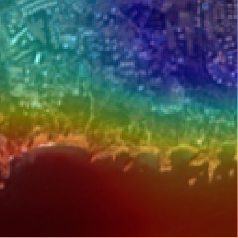
(a) Colorization                                                                                       L (luminosity)

      RGB                                                                                                Rec. error
                      Spectral Bands                                                                              ~
                                                                                                          ||ab – ab||1     Colorization
                           HxWx9

 (b) Fine-tuning                                                        (c) Ensemble
                                              Urban Fabric                                                                           Final
                                                                                                                                   prediction
                                              Agricoltural Land

                                                                                                                         AVERAGE
                                                                                 RGB
                                              Marine Waters

    Spectral                                  Broad-leaved Forest

     Bands
                                              Pastures

                                                                            Spectral bands

                            Fig. 1. An overview of the proposed pipeline for feature learning on satellite imagery.

                       IV. DATASETS                                      discriminated (e.g. non-irrigated arable land vs. permanently
   The two datasets we rely on data acquired through the                 irrigated land). For these reasons, in our experiments we adopt
Sentinel-2A and 2B satellites developed by the European                  the class-nomenclature proposed in [39], which reduces the
Space Agency (ESA). These satellites provide a multi-spectral            number of classes to 19. Moreover, we discard the 70 987
imagery over the earth with 12 spectral bands (covering the              patches displaying lands that are fully covered by clouds, cloud
visible, near and short wave infrared part of the electromag-            shadows, and seasonal snow.
netic spectrum) at three different spatial resolutions (10, 20
and 60 meters per pixel).                                                B. West Nile Disease Dataset
A. Land-cover classification - BigEarthNet                                  In the last decade, numerous studies have examined the
   In Remote Sensing, the main bottleneck in the adoption                complex interactions among vectors, hosts, and pathogens [3],
of deep networks was the lack of a large training set. In-               [40]. In particular, one of the major threat worldwide studied
deed, existing datasets (as Eurosat [35], PatterNet [36], UC             is represented by West Nile Disease (WND), a mosquito-
Merced Land Use Dataset [37]) include a small number of                  borne disease caused by West Nile virus (WNV). Mosquitoes
annotated images, hence resulting inadequate for training very           presence and abundance have been extensively proved to be
deep networks. To overcome this problem, [12] introduces                 associated with climatic and environmental factors such as
BigEarthNet, a novel large scale dataset collecting 590 326              temperatures, vegetation, rainfall [40]–[42], and remote sens-
tiles. Each example comprises of 12 bands (RGB included) and             ing has been an important key source for data collection. Our
multiple land-cover classes (provided by the CORINE Land                 capacity to collect and store data continues to expand rapidly
Cover (CLC) database [38]) as ground truth.                              and this requires the incorporation of new analytical techniques
   Originally, the number of classes amounted to 43: but, the            able to process Earth Observation (EO) data establishing
authors of [39] argue that some CORINE classes cannot be                 pipelines to turn near real-time big data into smart data [43].
easily inferred by looking at Sentinel-2 images solely. Indeed,          In this context, Deep techniques could provide useful tools
some labels may not be recognizable at such low resolution               to process data and automatically identify patterns able to
(the highest one is 120 × 120 pixels for 10m bands) and other            make accurate predictions of the spatio-temporal re-emergence
ones would require temporal information for being correctly              and spread of the West Nile Disease in Italy. With this aim,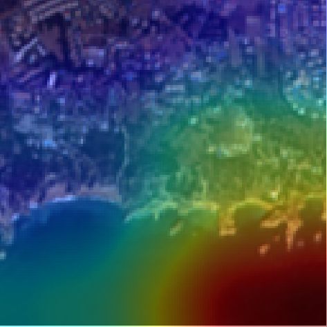
we collected data from the Copernicus program and paired                                         TABLE I
Sentinel 2 (S2) EO data with ground truth WND data.                 P ERFORMANCE ( M AP) ON B IG E ARTH N ET FOR DIFFERENT STRATEGIES
                                                                             TO VARY THE NUMBER OF TRAINING EXAMPLES .
   Disease sites are collected through the National Disease
Notification System of the Ministry of Health (SIMAN                   Input        pre-training    1k          5k        10k      50k       Full
www.vetinfo.sanita.it) [44]. We start with the analysis of
                                                                       RGB          from scratch    .486      .608      .645       .744      .851
the 2018 epidemic, one of the most spread on the Italian               RGB            ImageNet      .620      .695      .726       .786      .879
territory. We frame the problem as a binary classification
                                                                       Spectral     from scratch    .555      .667      .711       .767      .866
task with the final purpose of predicting positive and negative        Spectral       ImageNet      .578      .627      .681       .773      .879
WND sites analyzing multi-spectral bands. Positive cases are           Spectral     Color. (our)    .622      .730      .760       .793      .860
geographically located mainly in Po valley, in Sardinia and
some spots in the rest of Italy [45]: the location of each case
of birds, mosquitoes and horses, was visually inspected for the                                 TABLE II
accuracy needs in the analysis. Negative sites, being not always            E NSEMBLE MODEL – RESULTS ( M AP) ON B IG E ARTH N ET .
available in the national database due to the surveillance plan
strategy, were derived as pseudo-absence ground truth data,         Input            pre-training          1k        5k         10k       50k       Full
either in the space (points located in areas where the disease
                                                                    RGB               ImageNet             .620      .695       .726      .786      .879
was never reported in the past) and in the time (a random
date in months previous the reported positivity in mosquitoes       Spectral         Colorization          .622      .730       .760      .793      .860
collections).                                                       Ensemble      ImagNet+ImageNet         .649      .707       .749      .815      .904
   WND dataset comprises of 1 488 distinct cases, divided           Ensemble       Color.+ImageNet         .656      .751       .778      .823      .896
into 962 negatives and 526 positives. Each case comes with
a variable number of Sentinel-2 patches (corresponding to
various acquisitions over time), thus leading to 18 684 spectral   to outliers. Before feeding the spectral bands into the model
images in total.                                                   – as they come with different spatial resolutions – we apply a
                      V. E XPERIMENTS                              cubic interpolation to get a dimension of 128 × 128.
                                                                   Colorization. To broaden the diversity of available data, we
In this section, we test our proposal as a pre-training strategy   apply data augmentation (i.e. rotation, horizontal and, vertical
for the later fine-tuning step. We compare the results yielded     flip). We initialize the network according to [46] and train
by colorization to those achieved by two baselines: training       for 50 epochs on the full BigEarthNet, setting the batch size
from scratch [46] and the common ImageNet pre-training.            equal to 16 and leveraging Stochastic Gradient Descent (SGD)
In doing so, we mimic scenarios with few labeled data by           as optimizer (with a learning rate fixed at 0.01).
reducing the amount of examples available at training time
                                                                   Land-Cover Classification. We train the model for 30 epochs
(e.g. 1 000, 5 000, etc. . . ).
                                                                   whether the full dataset is available; otherwise we increase the
A. Evaluation Protocols                                            epochs to 50. The learning rate is set to 0.1 and divided by
                                                                   10 at the 10th and 40th epoch. The batch size equals 64.
Land-Cover Classification. We strictly follow the guidelines
                                                                   West Nile Disease Differently from the previous cases, we
provided by [11] when assessing the performance on the
                                                                   apply neither upscaling nor pixel-normalization, as all chan-
BigEarthNet benchmark. Namely, we form the training set
                                                                   nels are provided at the same resolution (224 × 224) and their
by sampling 60% of the total examples, retaining 20% for
                                                                   values lie within the range [0, 1]. We leverage the network
the validation set and 20% for the test set. We measure the
                                                                   trained for colorization on BigEarthNet. Since we rely on a
results in terms of Mean-Average-Precision (mAP), which also
                                                                   subset of the spectral bands (B1 , B8A , B11 and B12 ), we fix
considers the order in which predictions are given to the user.
                                                                   the first convolutional layer so that it takes 4 channels as input.
We check the performance every 10 epochs and retain the
                                                                   We optimize the model for 30 epochs, with a batch size of 32
weights that yield the higher mAP score on the validation set.
                                                                   and an initial learning rate of 0.001, multiplied by 0.1 after
West Nile Disease. Here, we adopt the stratified holdout
                                                                   25 epochs.
strategy, which ensures the class probabilities of training and
test being close to each other. The metrics of interest are
                                                                   C. Results of Colorization pre-training
precision, recall and F1 score, the latter accounting for the
slight imbalance that occurs at class level (indeed, negatives        Based on the final performance reported in Tab. I, one can
cases appear more frequently than positives ones).                 observe the initialization offered by colorization surpassing the
                                                                   other alternatives. Such a claim especially holds in presence
B. Implementation details                                          of scarce data, thus complying with the goals we have striven
BigEarthNet. We exploit the normalization technique de-            for in this work. This does not apply when the learner faces
scribed in [43], [47] computing the 2nd and 98th percentile        up to the entire training set (519k examples): such evidence
values to normalize each band. This method is more robust          – already encountered in [11] – deserves more investigations
than the common min-max normalization, as it is less sensitive     that we will conduct in future works.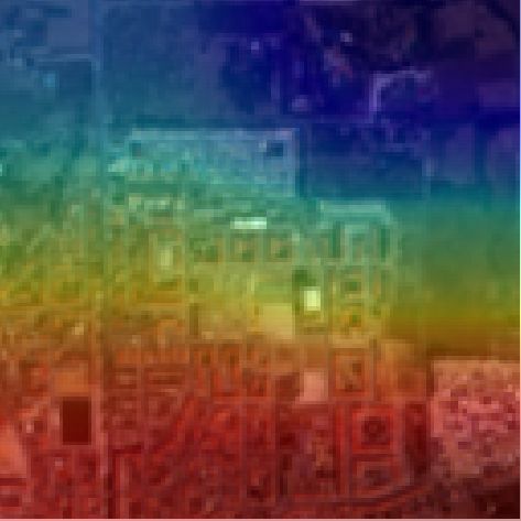
TABLE III Marine Coniferous
P ERFORMANCE ( ACC . ACCURACY, PR . PRECISION , RC . RECALL ) ON THE Urban fabric Arable land
waters forest
W EST N ILE D ISEASE CASE STUDY, FOR DIFFERENT METHODS AND
PRE - TRAINING STRATEGIES .
Input pre-training acc. pr. rc. F1
RGB
Real
Random
- .503 .391 .395 .393
classifier
RGB from scratch .652 .542 .941 .688
Predicted
RGB ImageNet .865 .819 .857 .838
B1,8A,11,12 from scratch .756 .662 .817 .732
RGB
B1,8A,11,12 Colorization .852 .823 .811 .817
Ensemble Color.+ImageNet .880 .855 .850 .852
Expl. RGB
branch
TABLE IV
C OMPARISON BETWEEN SEVERAL BASELINES AND OUR ENSEMBLE
METHOD ON B IG E ARTH N ET .
Method pr. rc. F1
Heat Spec.
K-Branch CNN [12] .716 .789 .727
branch
VGG19 [12] .798 .767 .759
ResNet-50 [12] .813 .774 .771
ResNet-101 [12] .801 .774 .764
ResNet-152 [12] .817 .762 .765
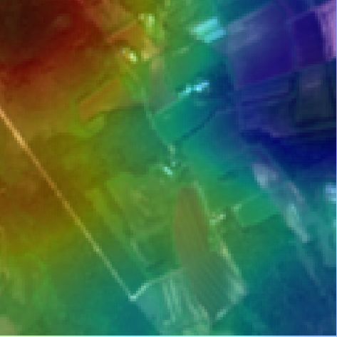
Fig. 2. Some examples of the BigEarthNet dataset, coupled with the predicted
Ensemble (our) 84.30 78.10 81.10
colorization and visual explanations provided by the ensemble method for
RGB and spectral inputs.
Results shown by Tab. I let us draw additional remarks: reported in Tab. IV confirm the above intuitions: the en-
i) as one would expect, the ImageNet pre-training performs semble we build upon ResNet-18 outperforms heavier and
good for an RGB input; however, when dealing with the overparametrized networks like ResNet-101 or ResNet-152.
spectral domain, even a random initialization outperforms it; Notably, we found a large improvement in precision, suggest-
ii) colorization is the sole that rewards the exploitation of ing that our proposal is capable of returning only the categories
spectral bands and justifies their usage in place of RGB. that are relevant to the semantics of the input tile.
It is noted the fairness of the comparisons above, as both
D. Results of the Model ensemble
our ensemble and the baselines leverage the same amount
Here, we primarily assess the effectiveness of the ensem- of information in input (namely, spectral bands and color
ble discussed in Sec. III-C on BigEarthNet. In this regard, channels). Nevertheless, an important difference subsists in the
Tab. II compares the performance that can be reached when way information is consumed: while [12] stacks both the input
leveraging a twofold source of information (RGB and spectral modalities to form a single input tensor, we distinguish two
bands): firstly, the ensemble model largely outperforms those independent paths that eventually cross in the output space.
that consider a single input modality; secondly, colorization This way, we can benefit from two different pre-training,
presents an improvement over the ImageNet pre-training. each one being devoted to its modality: the one offered by
Tab. III reports the results achieved on the West Nile colorization – which works well for spectral bands – and
Disease case study discussed in Sec IV-B. To provide a better the ImageNet one – which instead represents a natural and
understanding, we additionally furnish a simple baseline (i.e. reasonable choice for dealing with RGB images.
“random classifier”) that computes predictions by randomly
guessing from the class-prior distribution of the training set. F. Model Explanation - Towards diverse feature sets
As a first remark, all the networks we trained exceed random We believe the strength of our ensemble approach being
guessing, hence suggesting they effectively learned meaningful a result of the diversity among the individual learners. We
and suitable features for the problem at hand. Secondly, the investigate the truthfulness of such a claim from a model
ensemble model plays an important role even in this case, explanation perspective, questioning which information in the
surpassing networks based on a single modality by a consistent input makes our models arrive at their decisions [48]. In
margin. particular, we take advantage of GradCam [49] to assess
whether the two branches look for different properties within
E. Comparison with the state of the art their inputs. The third and fourth rows of Fig. 2 highlight
To further highlight the contributions of our proposal, we the input regions that have been considered important for
compare it with the networks discussed in [12]. Results predicting the target category (we limit the analysis to the class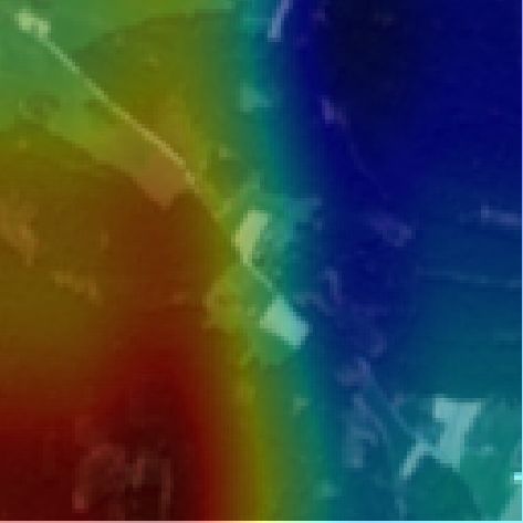
denoting the highest confidence score). As one can see, the                        [11] M. Neumann, A. S. Pinto, X. Zhai, and N. Houlsby, “In-domain repre-
explanations provided by the two branches visually diverge,                             sentation learning for remote sensing,” arXiv preprint arXiv:1911.06721,
                                                                                        2019.
thus qualitatively confirming the weak correlation between                         [12] G. Sumbul, M. Charfuelan, B. Demir, and V. Markl, “Bigearthnet: A
their representations.                                                                  large-scale benchmark archive for remote sensing image understanding,”
                                                                                        arXiv preprint arXiv:1902.06148, 2019.
                           VI. C ONCLUSION                                         [13] N. Jean, S. Wang, A. Samar, G. Azzari, D. Lobell, and S. Ermon,
                                                                                        “Tile2vec: Unsupervised representation learning for spatially distributed
   In this work, we propose a self-supervised learning approach                         data,” in Proceedings of the AAAI Conference on Artificial Intelligence,
for satellite imagery, which moves towards a proper initial-                            vol. 33, 2019, pp. 3967–3974.
                                                                                   [14] G. Larsson, M. Maire, and G. Shakhnarovich, “Colorization as a proxy
ization for deep networks facing up to Remote Sensing tasks.                            task for visual understanding,” in Proceedings of the IEEE Conference
Our proposal builds upon two steps: firstly, we ask an encoder-                         on Computer Vision and Pattern Recognition, 2017, pp. 6874–6883.
decoder architecture to predict color channels from those cap-                     [15] R. Zhang, P. Isola, and A. A. Efros, “Split-brain autoencoders: Unsu-
turing spectral information (colorization); secondly, we exploit                        pervised learning by cross-channel prediction,” in Proceedings of the
                                                                                        IEEE Conference on Computer Vision and Pattern Recognition, 2017,
its encoder as a pre-trained feature extractor for a classification                     pp. 1058–1067.
task (i.e. land-cover categorization and the West Nile Disease                     [16] K. Makantasis, K. Karantzalos, A. Doulamis, and N. Doulamis, “Deep
case study). We observe that the initialization we devised leads                        supervised learning for hyperspectral data classification through convo-
                                                                                        lutional neural networks,” in 2015 IEEE International Geoscience and
to remarkable results, exceeding the baselines especially in                            Remote Sensing Symposium (IGARSS). IEEE, 2015, pp. 4959–4962.
presence of scarce labeled data. Moreover, we qualitatively                        [17] R. Hang, Q. Liu, D. Hong, and P. Ghamisi, “Cascaded recurrent neural
observe that representations learned through colorization are                           networks for hyperspectral image classification,” IEEE Transactions on
                                                                                        Geoscience and Remote Sensing, vol. 57, no. 8, pp. 5384–5394, 2019.
different from the ones driven by the RGB channels. Based                          [18] Y. Li, H. Zhang, and Q. Shen, “Spectral–spatial classification of hyper-
on this finding, we set up an ensemble model that achieves                              spectral imagery with 3d convolutional neural network,” Remote Sensing,
the highest results in all the scenarios under consideration.                           vol. 9, no. 1, p. 67, 2017.
                                                                                   [19] D. Marmanis, M. Datcu, T. Esch, and U. Stilla, “Deep learning earth
                          ACKNOWLEDGMENT                                                observation classification using imagenet pretrained networks,” IEEE
                                                                                        Geoscience and Remote Sensing Letters, vol. 13, no. 1, pp. 105–109,
   The research described in this paper has been conducted                              2015.
within the project ‘AIDEO’ (AI and EO as Innovative Methods                        [20] K. Nogueira, O. A. Penatti, and J. A. Dos Santos, “Towards better
                                                                                        exploiting convolutional neural networks for remote sensing scene
for Monitoring West Nile Virus Spread). The project is being                            classification,” Pattern Recognition, vol. 61, pp. 539–556, 2017.
developed within the scope of the ESA EO Science for Society                       [21] X. Yu, X. Wu, C. Luo, and P. Ren, “Deep learning in remote sensing
Permanently Open Call for Proposals EOEP-5 BLOCK 4                                      scene classification: a data augmentation enhanced convolutional neural
                                                                                        network framework,” GIScience & Remote Sensing, vol. 54, no. 5, pp.
(ESA AO/1-9101/17/I-NB).                                                                741–758, 2017.
                                                                                   [22] L. Jing and Y. Tian, “Self-supervised visual feature learning with deep
                               R EFERENCES                                              neural networks: A survey,” arXiv preprint arXiv:1902.06162, 2019.
                                                                                   [23] P. Vincent, H. Larochelle, Y. Bengio, and P.-A. Manzagol, “Extract-
 [1] G. J. Schumann, G. R. Brakenridge, A. J. Kettner, R. Kashif, and
                                                                                        ing and composing robust features with denoising autoencoders,” in
     E. Niebuhr, “Assisting flood disaster response with earth observation
                                                                                        Proceedings of the 25th international conference on Machine learning,
     data and products: a critical assessment,” Remote Sensing, vol. 10, no. 8,
                                                                                        2008, pp. 1096–1103.
     p. 1230, 2018.
 [2] F. Filipponi, “Exploitation of sentinel-2 time series to map burned areas     [24] Z. Lin, Y. Chen, X. Zhao, and G. Wang, “Spectral-spatial classification
     at the national level: A case study on the 2017 italy wildfires,” Remote           of hyperspectral image using autoencoders,” in 2013 9th International
     Sensing, vol. 11, no. 6, p. 622, 2019.                                             Conference on Information, Communications & Signal Processing.
                                                                                        IEEE, 2013, pp. 1–5.
 [3] C. Ippoliti, L. Candeloro, M. Gilbert, M. Goffredo, G. Mancini, G. Curci,
     S. Falasca, S. Tora, A. Di Lorenzo, M. Quaglia et al., “Defining              [25] X. Ma, H. Wang, and J. Geng, “Spectral–spatial classification of hyper-
     ecological regions in italy based on a multivariate clustering approach:           spectral image based on deep auto-encoder,” IEEE Journal of Selected
     A first step towards a targeted vector borne disease surveillance,” PloS           Topics in Applied Earth Observations and Remote Sensing, vol. 9, no. 9,
     one, vol. 14, no. 7, 2019.                                                         pp. 4073–4085, 2016.
 [4] D. Rolnick, P. L. Donti, L. H. Kaack, K. Kochanski, A. Lacoste,               [26] S. Gidaris, P. Singh, and N. Komodakis, “Unsupervised repre-
     K. Sankaran, A. S. Ross, N. Milojevic-Dupont, N. Jaques, A. Waldman-               sentation learning by predicting image rotations,” arXiv preprint
     Brown et al., “Tackling climate change with machine learning,” arXiv               arXiv:1803.07728, 2018.
     preprint arXiv:1906.05433, 2019.                                              [27] C. Doersch, A. Gupta, and A. A. Efros, “Unsupervised visual repre-
 [5] M. Drusch, U. Del Bello, S. Carlier, O. Colin, V. Fernandez, F. Gascon,            sentation learning by context prediction,” in Proceedings of the IEEE
     B. Hoersch, C. Isola, P. Laberinti, P. Martimort et al., “Sentinel-2: Esa’s        International Conference on Computer Vision, 2015, pp. 1422–1430.
     optical high-resolution mission for gmes operational services,” Remote        [28] M. Noroozi and P. Favaro, “Unsupervised learning of visual representa-
     sensing of Environment, vol. 120, pp. 25–36, 2012.                                 tions by solving jigsaw puzzles,” in European Conference on Computer
 [6] S. Ji, Z. Chi, A. Xu, Y. Shi, and Y. Duan, “3d convolutional neural                Vision. Springer, 2016, pp. 69–84.
     networks for crop classification with multi-temporal remote sensing           [29] G. Larsson, M. Maire, and G. Shakhnarovich, “Colorization as a proxy
     images,” Remote Sensing, vol. 10, p. 75, 01 2018.                                  task for visual understanding,” in Proceedings of the IEEE Conference
 [7] G. Masi, D. Cozzolino, L. Verdoliva, and G. Scarpa, “Pansharpening by              on Computer Vision and Pattern Recognition, 2017, pp. 6874–6883.
     convolutional neural networks,” Remote Sensing, vol. 8, no. 7, p. 594,        [30] A. Deshpande, J. Lu, M.-C. Yeh, M. Jin Chong, and D. Forsyth,
     2016.                                                                              “Learning diverse image colorization,” in Proceedings of the IEEE
 [8] J. Sherrah, “Fully convolutional networks for dense semantic labelling of          Conference on Computer Vision and Pattern Recognition, 2017, pp.
     high-resolution aerial imagery,” arXiv preprint arXiv:1606.02585, 2016.            6837–6845.
 [9] M. Huh, P. Agrawal, and A. A. Efros, “What makes imagenet good for            [31] G. Larsson, M. Maire, and G. Shakhnarovich, “Learning representations
     transfer learning?” arXiv preprint arXiv:1608.08614, 2016.                         for automatic colorization,” in European Conference on Computer
[10] J. Deng, W. Dong, R. Socher, L.-J. Li, K. Li, and L. Fei-Fei, “Imagenet:           Vision. Springer, 2016, pp. 577–593.
     A large-scale hierarchical image database,” in 2009 IEEE conference on        [32] R. Zhang, P. Isola, and A. A. Efros, “Colorful image colorization,” in
     computer vision and pattern recognition. Ieee, 2009, pp. 248–255.                  European conference on computer vision. Springer, 2016, pp. 649–666.
[33] K. He, X. Zhang, S. Ren, and J. Sun, “Deep residual learning for image
     recognition,” in IEEE International Conference on Computer Vision and
     Pattern Recognition, 2016, pp. 770–778.
[34] A. Kolesnikov, X. Zhai, and L. Beyer, “Revisiting self-supervised visual
     representation learning,” in Proceedings of the IEEE conference on
     Computer Vision and Pattern Recognition, 2019, pp. 1920–1929.
[35] P. Helber, B. Bischke, A. Dengel, and D. Borth, “Eurosat: A novel
     dataset and deep learning benchmark for land use and land cover classi-
     fication,” IEEE Journal of Selected Topics in Applied Earth Observations
     and Remote Sensing, vol. 12, no. 7, pp. 2217–2226, 2019.
[36] W. Zhou, S. Newsam, C. Li, and Z. Shao, “Patternnet: A benchmark
     dataset for performance evaluation of remote sensing image retrieval,”
     ISPRS journal of photogrammetry and remote sensing, vol. 145, pp.
     197–209, 2018.
[37] Y. Yang and S. Newsam, “Bag-of-visual-words and spatial extensions
     for land-use classification,” in Proceedings of the 18th SIGSPATIAL in-
     ternational conference on advances in geographic information systems,
     2010, pp. 270–279.
[38] J. Feranec, T. Soukup, G. Hazeu, and G. Jaffrain, European landscape
     dynamics: CORINE land cover data. CRC Press, 2016.
[39] G. Sumbul, J. Kang, T. Kreuziger, F. Marcelino, H. Costa, P. Benevides,
     M. Caetano, and B. Demir, “Bigearthnet deep learning models with a
     new class-nomenclature for remote sensing image understanding,” arXiv
     preprint arXiv:2001.06372, 2020.
[40] A. Tran, B. Sudre, S. Paz, M. Rossi, A. Desbrosse, V. Chevalier, and J. C.
     Semenza, “Environmental predictors of west nile fever risk in europe,”
     International journal of health geographics, vol. 13, no. 1, p. 26, 2014.
[41] D. Bisanzio, M. Giacobini, L. Bertolotti, A. Mosca, L. Balbo, U. Kitron,
     and G. M. Vazquez-Prokopec, “Spatio-temporal patterns of distribution
     of west nile virus vectors in eastern piedmont region, italy,” Parasites
     & vectors, vol. 4, no. 1, p. 230, 2011.
[42] A. Conte, L. Candeloro, C. Ippoliti, F. Monaco, F. De Massis, R. Bruno,
     D. Di Sabatino, M. L. Danzetta, A. Benjelloun, B. Belkadi et al.,
     “Spatio-temporal identification of areas suitable for west nile disease in
     the mediterranean basin and central europe,” PloS one, vol. 10, no. 12,
     2015.
[43] S. Vincenzi, A. Porrello, P. Buzzega, A. Conte, C. Ippoliti, L. Candeloro,
     A. Di Lorenzo, A. C. Dondona, and S. Calderara, “Spotting insects
     from satellites: modeling the presence of culicoides imicola through
     deep cnns,” arXiv preprint arXiv:1911.10024, 2019.
[44] P. Colangeli, S. Iannetti, A. Cerella, C. Ippoliti, and A. Di, “Sistema
     nazionale di notifica delle malattie degli animali,” Veterinaria Italiana,
     vol. 47, no. 3, pp. 291–301, 2011.
[45] F. Riccardo, F. Monaco, A. Bella, G. Savini, F. Russo, R. Cagarelli,
     M. Dottori, C. Rizzo, G. Venturi, M. Di Luca et al., “An early start
     of west nile virus seasonal transmission: the added value of one heath
     surveillance in detecting early circulation and triggering timely response
     in italy, june to july 2018,” Eurosurveillance, vol. 23, no. 32, 2018.
[46] K. He, X. Zhang, S. Ren, and J. Sun, “Delving deep into rectifiers:
     Surpassing human-level performance on imagenet classification,” in
     Proceedings of the IEEE international conference on computer vision,
     2015, pp. 1026–1034.
[47] G. Prathap and I. Afanasyev, “Deep learning approach for building detec-
     tion in satellite multispectral imagery,” in 2018 International Conference
     on Intelligent Systems (IS). IEEE, 2018, pp. 461–465.
[48] W. Samek, T. Wiegand, and K.-R. Müller, “Explainable artificial in-
     telligence: Understanding, visualizing and interpreting deep learning
     models,” arXiv preprint arXiv:1708.08296, 2017.
[49] R. R. Selvaraju, M. Cogswell, A. Das, R. Vedantam, D. Parikh,
     and D. Batra, “Grad-cam: Visual explanations from deep networks
     via gradient-based localization,” in IEEE International Conference on
     Computer Vision and Pattern Recognition, 2017.
You can also read