CAMERAS: Enhanced Resolution And Sanity preserving Class Activation Mapping for image saliency
←
→
Page content transcription
If your browser does not render page correctly, please read the page content below
CAMERAS: Enhanced Resolution And Sanity preserving Class Activation
                                                               Mapping for image saliency

                                               Mohammad A. A. K. Jalwana Naveed Akhtar Mohammed Bennamoun Ajmal Mian
                                                  Computer Science and Software Engineering, The University of Western Australia.
                                            {mohammad.jalwana@research., naveed.akhtar@, mohammed.bennamoun@, ajmal.mian@}uwa.edu.au
                                                                              Code:      https://github.com/VisMIL/CAMERAS
arXiv:2106.10649v1 [cs.CV] 20 Jun 2021

                                                                  Abstract                                      Addressing this issue for deep visual models, tech-
                                                                                                            niques are emerging to offer input-agnostic [11] and input-
                                             Backpropagation image saliency aims at explaining
                                                                                                            specific [8], [21], [25] explanation of model predictions.
                                         model predictions by estimating model-centric impor-
                                                                                                            This work subscribes to the latter, where the ultimate goal
                                         tance of individual pixels in the input. However, class-
                                                                                                            is to identify the contribution of each pixel in an input to
                                         insensitivity of the earlier layers in a network only allows
                                                                                                            the output prediction. The popular techniques to achieve
                                         saliency computation with low resolution activation maps of
                                                                                                            this adopt one of two strategies. The first, systematically
                                         the deeper layers, resulting in compromised image saliency.
                                                                                                            modifies the input image pixels (i.e. image regions) and an-
                                         Remedifying this can lead to sanity failures. We propose
                                                                                                            alyzes the effects of those perturbations on the output pre-
                                         CAMERAS, a technique to compute high-fidelity backprop-
                                                                                                            dictions [8], [9], [20], [33]. The underlying search nature
                                         agation saliency maps without requiring any external priors
                                                                                                            of this perturbation-based formulation offers high-fidelity
                                         and preserving the map sanity. Our method systematically
                                                                                                            model-centric importance attribution to the input pixels, al-
                                         performs multi-scale accumulation and fusion of the acti-
                                                                                                            beit at a high computational cost. Hence, tractability is
                                         vation maps and backpropagated gradients to compute pre-
                                                                                                            achieved under heuristics or external priors over the com-
                                         cise saliency maps. From accurate image saliency to artic-
                                                                                                            puted importance maps. This is undesired because the
                                         ulation of relative importance of input features for different
                                                                                                            eventual maps may be influenced by these external factors,
                                         models, and precise discrimination between model percep-
                                                                                                            which compromises the model-fidelity of the maps.
                                         tion of visually similar objects, our high-resolution map-
                                         ping offers multiple novel insights into the black-box deep            The second strategy relies on the activation maps of the
                                         visual models, which are presented in the paper. We also           internal layers and gradients of the models. Commonly
                                         demonstrate the utility of our saliency maps in adversarial        known as backpropagation saliency methods [25], [21],
                                         setup by drastically reducing the norm of attack signals by        [27], [30], [33], [34] approaches adopting this strategy are
                                         focusing them on the precise regions identified by our maps.       computationally efficient, thereby offering the possibility
                                         Our method also inspires new evaluation metrics and a san-         of avoiding unnecessary heuristics or priors. However, for
                                         ity check for this developing research direction.                  the visual neural models, the layers closer to the input are
                                                                                                            class-insensitive [21]. This limits the ammunition of back-
                                                                                                            propagation saliency methods to the deeper layers of the
                                         1. Introduction                                                    networks, where the size of activation maps is very small,
                                            Deep visual models are fast surpassing human-level per-         e.g. 10−3 × of the input size. Projecting the saliency com-
                                         formance for various vision tasks, including image classifi-       puted with those maps onto the original image grid results
                                         cation [15], [28], object detection [22], [23], and semantic       in intrinsically low-resolution image saliency. On the other
                                         segmentation [17], [5]. However, they hardly offer any ex-         hand, using heuristics or priors to sharpen those projections
                                         planation of their decisions, and are rightfully considered        inadvertently compromise the sanity of the maps [2]. Not to
                                         black-boxes. This is problematic for their practical deploy-       mention, employing activation signals of multiple internal
                                         ment, especially in high-risk emerging applications where          layers for resolution enhancement takes us back to a combi-
                                         transparency is vital, e.g. in healthcare, self-driving vehicles   natorial search problem of choosing the best layers, under a
                                         and smart surveillance [21]. The problem is exacerbated            pre-specified heuristic.
                                         by the push of ‘right to explanation’ by algorithmic regula-           Addressing the above issues, we introduce CAMERAS
                                         tory authorities and their objection to black-box models in        - an Enhanced Resolution And Sanity preserving Class
                                         safety-critical applications [1].                                  Activation Mapping for backpropagation image saliency.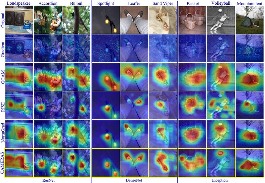
Figure 1. (Top) CAMERAS meticulously fuses activation maps and backpropagated gradients of a layer for multi-scale copies of an input.
After passing the resulting saliency map through ReLU and normalising it (f ), the map is embedded on the original image. (Bottom) By
avoiding influence of external factors, CAMERAS easily passes the sanity checks for image saliency. Shown are the results of cascading
randomization [2] on ResNet. Progressive randomising of layer weights randomises the output right from the logits layer which identifies
preservation of sanity. Thus, the CAMERAS maps do not sacrifice their sanity for high-resolution, achieving the best of both worlds.

The proposed technique (Fig. 1-top) systematically accu-                    PGD [18] with our saliency technique - drastically im-
mulates and fuses multi-scale activation maps and back-                     proving the efficacy of the attack.
propagated gradients of a model to construct precise                      • The ability of precise saliency computation allowed by
saliency maps. By avoiding the influence of any exter-                      CAMERAS calls for new quantitative metrics and san-
nal factor, e.g. heuristics, priors, thresholds, the saliency               ity checks. We contribute two new evaluation metrics
maps of CAMERAS easily pass the sanity checks for im-                       and a sanity check to advance this research direction.
age saliency (Fig. 1-bottom). Moreover, the technique al-
lows saliency estimation with a single network layer, not
requiring any layer search for map resolution enhancement.             2. Related work
Contributions of the paper are summarised below:                           The literature has seen multiple techniques that perturb
                                                                       input pixels and measure its effects on the model outputs
   • We propose CAMERAS for precise backpropagation
                                                                       to identify salient regions in input images [9], [8], [20].
     image saliency while preserving the sanity. Our
                                                                       Perturbing every possible combination of pixels has an ex-
     method outperforms the state-of-the-art saliency meth-
                                                                       ponential complexity. Therefore, such techniques often
     ods by a large margin, achieving up to 27.5% error re-
                                                                       rely on fixed subsets of pixel combinations for tractabil-
     duction for the popular pointing game metric [34].
                                                                       ity. Moreover, high non-linearity of deep models further
   • Exploring the newly found precision saliency map-                 restricts the saliency map to be reliable under fixed de-
     ping with CAMERAS, we visualise differences in the                vised perturbation subsets. RISE [20] and Occlusion [33]
     semantic understanding of different architectures that            generate attribution maps by weighing perturbation masks
     govern their performance. We also highlight model-                corresponding to the changes in the output scores. Other
     centric discrimination of input features for visually             techniques, such as Meaningful perturbations [9], Extremal
     similar objects in never-before-seen details.                     perturbations [8], Real-time saliency [6] and [24] cast the
   • Considering the equivalent treatment of deep mod-                 problem into an optimization objective. Though effective,
     els as differentiable programs by the fast-developing             these methods face a common issue of allowing a channel
     parallel field of adversarial learning, we enhance                for external influence on the resulting maps in the form of
     the widely considered strongest adversarial attack                e.g. heuristics, external constraints, priors or threshold etc.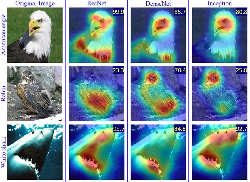
Backpropagation saliency methods [27], [25], [33] aim         3. Proposed Approach
at extracting information from within the model to identify          Before discussing the details of our technique, we first
model-centric salient regions in an input image. Relying          provide a closer look at the broader paradigm of backprop-
on layer activations and model gradients, these methods are       agation saliency computation. We use Grad-CAM [25] - a
also known to be computationally more effective [36], [12].       popular technique - as a test case to motivate the proposed
Simoyan et al. [27] first used model gradients as a possi-        method. The text below highlights only the relevant aspects
ble explanation of output predictions. Different adaptations      of the test case for intuition.
have since been proposed to mitigate the inherent noise sen-
sitivity of model gradients. Guided back prop [30] and            3.1. Saliency computation with backpropagation
DeConvNet [33] alter the backpropagation rules of model               Let I ∈ Rc×h×w be an input image with ‘c’ channels.
ReLU layers, while SmoothGrad [29] computes the aver-             A deep visual classifier K(I) maps I to a prediction vector
age gradients over samples in the close vicinity of the origi-    y ` ∈ RL , where ‘L’ is the total number of classes. Here, ‘`’
nal one. Similarly, DeepLIFT [26], LRP [4] and Excitation         indicates the predicted label of I under the premise that the
Backprop [34] recast the backpropagation rules such that          `th coefficient of y has the largest value. It is well-known
the sum of attribution signal becomes unity. Sundararajan et      that a neural network is a hierarchical composition of rep-
al. [31] interpolated multiple attribution maps to reduce the     resentation layers. Rebuffi et al. [21] demonstrated that
signal noise. There are also instances of exploring saliency      among these layers, those closer to the input learn class-
computation using various layers of deep models by merg-          insensitive features. Thus, the deeper layers hold more
ing the layer activation maps with the gradient information.      promise for computing image saliency for a model. Grad-
Such methods include CAM [35], its generalized adaption           CAM [25] takes a pragmatic approach to single out the last
GradCAM [25], linear approximation [14] and NormGrad              convolutional layer to estimate the saliency map.
[21]. For such methods, it is found that the layers closer to         Let us denote the k th activation map of the last convo-
output generate better saliency maps because those layers         lutional layer of a network as Ak (I) ∈ Rm×n . Focusing
are more sensitive to the high level class features.              on Grad-CAM, the technique first computes an intermedi-
   Beyond the visual quality of saliency maps, a few works        ate representation S(I) ∈ Rm×n , such that S (i,j) (I) =
                                                                  P         (i,j)
have also critically explored the reliability of these maps for      k w k Ak     (I), where wk is given by Eq. (1). Henceforth,
different methods [19], [13]. Adebayo et al. [2] first intro-     we ignore the argument (I) for clarity, unless required.
duced sanity checks for image saliency methods, highlight-                                      m X  n
                                                                                                                  !
ing that visual appeal of the maps alone can be misleading.                              1     X            ∂y `
                                                                              wk =                                   .       (1)
They evaluated sensitivity of the results of popular tech-                            (m + n) i=1 j=1 ∂A(i,j)
                                                                                                            k
niques to model parameters. Surprisingly, ‘model-centric
saliency maps’ computed by multiple methods were found            In the above expressions, X (i,j) is the (i, j) coefficient of
insensitive to the model - failing the sanity check. The tech-    X. The computed S is later extended to the final saliency
niques avoiding external influences on the map, e.g. Grad-        map Ψ ∈ Rh×w , as f (S) : S → Ψ, where the function
CAM [25] easily passed the test. This finding also resonated      f (.) must account for interpolating an m × n matrix for a
with other subsequent sanity checks [21].                         h × w grid (along other complementary transformations).
    Evaluation of image saliency methods is a challenging
problem because deep model representation is not always           3.2. Sub-optimality of backpropagation methods
aligned with the human visual system [32]. Hence, indi-              Observing Grad-CAM (and similar methods) from the
rect evaluation of image saliency is often done by analysing      above perspective reveals two performance drain-holes in
its weak localization performance. For instance, Pointing         backpropagation image saliency computations.
game score [34] is a commonly used metric for quantitative        (a) Over-simplification of the weights wk : Since Ak is an
evaluation of image saliency results [8], [21]. It measures       activation map, individual coefficients of this matrix should
the correlation between the maximal point in a saliency map       have different importance for the final prediction. Indeed,
with the semantic labels of the pixel. Its later adaptation [9]   this is also reflected in the values of individual backpropa-
measures the overlap in the bounding boxes from saliency          gated gradients for these coefficients - computed with the
maps and the ground truth. Petsiuk et al. [20] proposed           expression in the parenthesis in Eq. (1). Since the ul-
insertion-deletion metrics to measure the impact of pertur-       timate objective of image saliency is to compute impor-
bations over image patches in the order of importance to          tance of individual pixels, loosing information with over-
quantify saliency accuracy. Nevertheless, these metrics are       simplification of wk is not conducive. Grad-CAM takes an
meant to be weak indicators of saliency maps due to the im-       extreme approach of representing wk with a scalar value.
precise nature of the maps computed by the earlier methods,       The main reason for that is, it is actually detrimental to
which is no longer the case for CAMERAS.                          plainly replace wk with an encoding W k ∈ Rm×n such that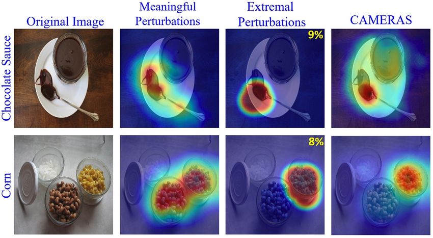
P
S = k W k Ak . Here, is the point-wise product and                 3.4. CAMERAS
W k encodes individual backpropagated gradients. Gradi-               Building directly on the insights in § 3.3, we devise
ents are extremely sensitive to signal variations. Hence,          CAMERAS - an enhanced resolution and sanity preserv-
even a small activation change can result in (a mislead-           ing class activation mapping scheme. The approach is il-
ing) exaggerated weight alteration for the activation map,         lustrated in Fig. (1-top) and explained below in a top-down
resulting in incorrect image saliency. Grad-CAM is able to         manner, keeping the flow of the above discussion.
mitigate this problem by averaging the gradients in Eq. (1).          Our method eventually computes a saliency map as:
However, this remedy comes at the cost of loosing the fine-                                                    !
grained information about the gradients.                                                       X ∗         ∗
                                                                              Ψ = f ReLU           Wk Ak , ∀k,              (2)
    Though centered around Grad-CAM, the above discus-
                                                                                                k
sion points to a simple, yet powerful generic notion for ef-
fective backpropagation saliency computation. That is, to                   ∗
                                                                   where Wk ∈ Rh×w encodes the differential information
better leverage the backpropagated gradients, the differen-
                                                                   of the backpropagated gradients for the k th activation map
tial information of the gradients (in W k ) is still at our dis-                            ∗
posal to exploit. Fusing activation maps with this informa-        in a network layer, Ak ∈ Rh×w is an enhanced resolution
tion promises more precise image saliency.                         encoding for the activation map itself, and f (.) performs an
                                                                                                                            ∗
(b) Large interpolated segments: Typically, the activation         element-wise normalisation in the range [0, 1]. The Wk and
maps of the deeper convolutional layer in visual classifiers        ∗
                                                                   Ak are defined as follows
are (spatially) much smaller than the input images. For in-
stance, in ResNet [10], the 7 × 7 maps of the last convo-                        ∗
                                                                                Wk = E ϕt W k (ϕt (I, ζt )), ζo ,               (3)
lutional layer are 1024 times smaller than the 224 × 224                                t
inputs. Thus, for m  h and n  w, a saliency map                                 ∗
                                                                                 Ak   = E ϕt Ak (ϕt (I, ζt )), ζo ,
Ψ computed with the class sensitive deeper layers must be                                   t
mainly composed of interpolated segments. To contextual-
                                                                   where ϕt (X, ζt ) is the tth up-sampling applied to resize X
ize, in the above ResNet example, 99.9% of the values are
                                                                   to the dimensions ζt - provided as a tuple. We fix ζo =
generated by the function f (S) : S → Ψ in Grad-CAM.
                                                                   (h, w) for I ∈ Rc×h×w . This will be explained
                                                                                                               shortly. We
This automatically renders Ψ a low-resolution map, leaving
                                                                                                                   ∂y `
alone the issue of correctness of the importance assigned          compute the (i, j) coefficient of W k as         (i,j)   . The
                                                                                                                  ∂Ak
to the individual pixels in the eventual saliency map. The
                                                                   overall process of generating an image saliency map with
low resolution of saliency maps has also spawned methods
                                                                   CAMERAS is summarized as Algorithm 1.
to improve f (.) [2], [25]. However, those techniques in-
                                                                      The algorithm computes the desired saliency map Ψ by
evitably rely on external information (including heuristics)
                                                                   an iterative multi-scale accumulation of activation maps and
for the transform S → Ψ due to unavailability of further
                                                                   gradients for the κth layer of the model. In the tth iteration,
useful information from the model itself. This leads to san-
                                                                   the input image I gets up-sampled to ζt based on the max-
ity check failures because the operands are no longer purely
                                                                   imum desired size ζm and the number of steps N allowed
grounded in the original model.
                                                                   to reach that size (lines 4,5). Provided that the input up-
3.3. The room for improvement                                      scaling does not alter the model prediction, the activation
   From the above discussion, it is clear that whereas use-        maps and backpropagated gradients to the κth layer are also
ful techniques exist for backpropagation image saliency, the       up-sampled and stored. We show this on lines 6-10 of the al-
paradigm is yet to fully harness the backpropagated gradi-         gorithm. Notice that, we use calligraphic symbols to distin-
ents and resolution enhancement of the activation maps for         guish 3D tensors from matrices (e.g. A instead of A for ac-
precise image saliency. Both limitations are rooted in the         tivations) in the algorithm for clarity. The newly introduced
very nature of the underlying signals. Leveraging these sig-       symbol ∇J (κ, `) on line 9 denotes the collective backprop-
nals from multiple layers can potentially help in partially        agated gradients to the κth layer w.r.t. the predicted label
overcoming the issues. However, this possibility is also           `. Also notice, on lines 8, 9, up-sampling of the activa-
restricted by the class-insensitivity of the earlier network       tion maps and gradients are performed to match the original
layers and combinatorial nature of the problem. Moreover,          image size ζo . This is because, the same accumulated sig-
there is evidence that multi-layer fusion can often adversely      nals are eventually transformed into the saliency map of the
affect image saliency [21]. Hence, a technique specifically        original image. We iteratively accumulate the up-sampled
targeting the class-sensitive last layer, while allowing min-      activation maps and gradients, and finally compute their av-
imal loss of differential information across backpropagated        erages on lines 12 and 13. On line 14, we compute the
gradients and improving activation map upsampling, holds           saliency map by solving Eq. (2). Here, matrix notation is
significant promises for better saliency computation.              intentionally used to match the original equation.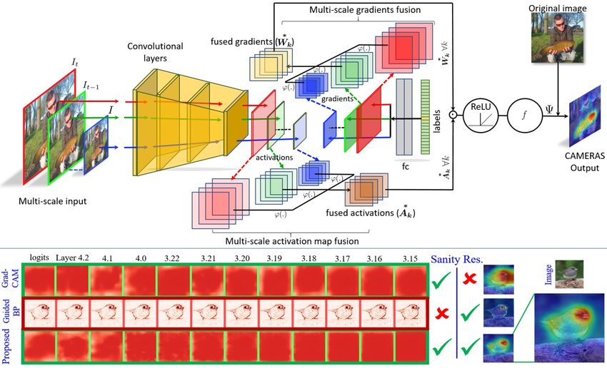
Algorithm 1 CAMERAS algorithm                                     resulting in low-resolution saliency maps. In CAMERAS,
Input: Classifier K, image I ∈ R      c×h×w
                                            , maximum size        the only source of any ‘potential’ external influence on the
    ζm , steps N , interpolation function ϕ(.), layer κ           resulting map is through the interpolation function ϕ(.). We
Output: Image saliency map Ψ ∈ Rh×w                               conjecture that as long as ϕ(.) is a first-order function de-
 1: Initialize Ao , Wo to 0 tensors, ζo = (h, w) and t =          fined over the signals originating in the model itself, CAM-
    tm = 0, ` = K(I)                                              ERAS maps will always preserve their sanity because the
 2: while t ≤ N do                                                maps would fully originate in the model. To preclude any
 3:    t←t+1                                                      unintentional prior over the maps, our formulation dictates
 4:    ζt ← ζt−1 + b ζNm c(t − 1)                                 the use of simpler functions as ϕ(.). Hence, we choose to
 5:    I t ← ϕt (I, ζt )                                          fix bi-linear interpolation as ϕ(.).
 6:    if K(I t ) → ` then                                            To analyse the reasons of extraordinary performance of
 7:       tm ← tm + 1                                            CAMERAS (see § 4), we provide a brief theoretical per-
 8:       At ← At−1 + ϕt A(I t , κ), ζo                          spective on the accumulation of multi-scale interpolated
 9:       Wt ← Wt−1 + ϕt ∇J (κ, `), ζo                            signals exploited by our method, using the results below.
10:    end if                                                                          ∗
                                                                  Lemma 3.1: For X ∈ Rh×w and its interpolated approx-
11: end while                                                                                                   ∗
     ∗                                                                    f = ϕ(X) s.t. X ∈ Rm×n and X 6= X,
12: A ← At /tm
                                                                  imation X                                             f
                                                                    ∗
      ∗
    W←W                                                           ||X − X||
                                                                        f = f ((h − m), (w − n)) for m < h and n < w,
13:      t /tm                                                  where ϕ(.) denotes bi-linear interpolation and f (.) is a
                P ∗                ∗
14: Ψ = f ReLU( k Wk              Ak )    , ∀k                    monotonic function over its arguments.
15:   return                                                      Lemma 3.2: For Xfz = ϕ(X z ), where X z ∈ Rm×n and
                                                                  fp = ϕ(X p ), where X p ∈ Rp×q s.t. p < m and n < q,
                                                                  X
                                                                    ∗               ∗
    In Algorithm 1, CAMERAS is shown to expect four
                                                                  ||X − X
                                                                        fz || − ||X − X
                                                                                      fp || ≤ 0.
input parameters, along with the classifier and the image.
                                                                                   ∗                ∗
We discuss the choice of ϕ(.) in § 3.4.1 where we even-           Corollary: E[||X − X
                                                                                     fz ||] ≤ ||X − X
                                                                                                    fp ||, ∀X
                                                                                                            fz ∪ X
                                                                                                                 fp .
                                                                              z
tually propose to keep this function fixed. The algorithm
optionally allows κ for computing saliency maps using lay-        The lemma 3.1 states that bi-linear interpolation tends to be
ers other than the last convolutional layer of the model. For     more accurate when the difference in the dimensions of the
all the experiments presented in the main paper, we keep κ        source signal and the target grid is smaller. The lemma 3.2
fixed to the last convolutional layer. This is due to the well-   can also be easily verified as Xfz is at least as accurate a
                                                                                 ∗
known class-sensitivity of the deeper layers of CNNs [21].        projection of X as X fp , according to lemma 3.1. This nec-
Essentially, the only choice to be made is for the values of      essarily makes its error equal to or smaller than the error
parameters ζm and N , which are related as ζm = cN ζo ,           of X
                                                                     fp . In the light of lemma 3.2, the corollary affirms that
where c is the step size. Trading-off performance with ef-        the expected error of a set of interpolated signals is upper-
ficiency, the choice of these parameters is mainly governed       bounded by the error of the least accurate signal in the set.
by the available computational resources. For larger ζm and
                                                                     The above analysis highlights an important aspect. The
N values, performance of CAMERAS roughly improves
                                                                  CAMERAS results will necessarily be as accurate as op-
monotonically - generally saturating at ζm ≈ (1K, 1K) for
                                                                  erating our algorithm on the original input size, and will
ζo = (224, 224) for the popular ImageNet models. For
                                                                  improve monotonically thereof with the up-sampled inputs.
this ζm range, the performance is largely insensitive for
                                                                  This is because the activations and gradients of the up-
N ∈ [5, 10]. We give further analysis of parameter values in
                                                                  sampled inputs would map more accurately on the original
the supplementary material. In the presented experiments,
                                                                  image grid, as per the above results. This is significant be-
we empirically choose ζm = (1K, 1K) and N = 7.
                                                                  cause it allows CAMERAS to use the differential informa-
3.4.1 Sanity preservation and strength                            tion in the backpropagated gradient maps while accounting
In CAMERAS, we do not impose any prior over the                   for the noise-sensitivity of the gradients by averaging out
saliency map, nor we use any heuristic to guide its com-          these signals across multiple scales. This is the key strength
putation process. The technique also preserves model fi-          of the proposed technique.
delity by requiring no structural (or any other) alteration
to the original model. It mainly relies on primitive arith-       4. Evaluation
metic operations over the model signals. These attributes            We perform a thorough qualitative and quantitative eval-
also characterize those other methods that pass the popular       uation of CAMERAS on large-scale models and compare
sanity checks for backpropagation saliency [2], [21], albeit      the performance with the state-of-the-art methods.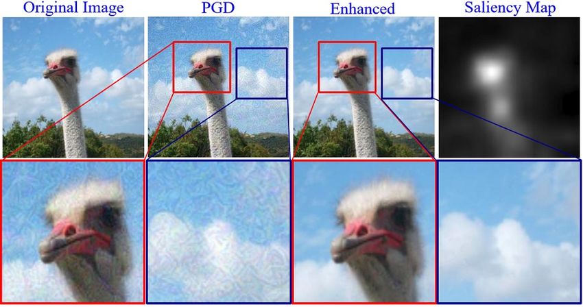
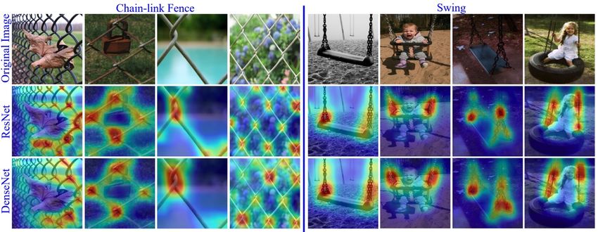
Figure 2. Visual comparison of saliency maps with the state-of-the-art methods. Representative maps are shown for random class images
for ResNet-50, DenseNet-121 and Inception-v3. Class labels are provided at the top. Results of proposed CAMERAS are in yellow box.

4.1. Qualitative results                                             ically evaluated by measuring their correlation with the se-
   In Fig. 2, we qualitatively compare the results of our            mantic annotations of the image. Pointing game [34] is a
technique with the existing saliency methods for ImageNet            popular metric for that purpose, which considers the com-
models of ResNet, DenseNet and Inception. Representa-                puted saliency for every object class in the image. If the
tive maps of randomly chosen images are provided. See                maximal point in the saliency map is contained within the
the supplementary material for more visualisations. The              object, it is considered a hit; otherwise, a miss. The perfor-
high quality of CAMERAS maps is apparent in the fig-                 mance is measured as the percentage of successful hits. We
ure. A quick inspection reveals that our technique main-             refer to [34] for more details on the metric. Table 1 bench-
tains its performance across a variety of scenarios, includ-         marks the performance of CAMERAS for pointing game
ing clear objects (Loudspeaker, Mountain tent), occluded             on 4, 952 images of PASCAL VOC test set [7], and ∼ 50K
objects (Bulbul), and multiples instances of objects (Accor-         images of COCO 2014 validation set [16]. Our technique
dion, Basket). Observing carefully, CAMERAS maps pro-                consistently shows superior performance, achieving up to
vide precise maps even for small and relatively complex ge-          27.5% error reduction. The gain is higher for ResNet as
ometric shapes, e.g. Volleyball, Spotlight, Loafer, Hognose          compared to VGG due the better performance of the origi-
snake. Interestingly, our method is able to attach appropri-         nal ResNet that permits better saliency.
ate importance even to the reflection of the Hognose snake.              The pointing game generally disregards precision of the
Adoption of saliency maps to complex geometric shapes is             saliency maps by focusing only on the maximal points. Ar-
a direct consequence of enabling precise saliency mapping            guably, crudeness of the saliency maps computed by the ear-
while sealing-off any external influence on the maps. CAM-           lier methods influenced this evaluation metric. The possibil-
ERAS is able to maintain its characteristic precision across         ity of precise saliency computation (by CAMERAS) calls
different models and images. These are highly promising              for new metrics that account for the finer details of saliency
results for explainability of modern deep visual classifiers.        maps. We propose ‘positive map density’ and ‘negative
4.2. Quantitative results                                            map density’ as two suitablePmetrics,     respectively defined
                                                                     as: ρ+                  Ψ))/ i j Ψ(i,j) × (h × w), and
                                                                                                        P
   A quantum leap in performance with CAMERAS is also                      map = P (K(I
                                                                     ρ−                  1 − Ψ))/ i j (1 − Ψ(i,j) ) × (h × w).
                                                                                                   P P
observed in our quantitative results. Saliency maps are typ-           map = P (K(I
VOC07 Test (All/Diff) COCO14 Val (All/Diff)
Method VGG16 ResNet50 VGG16 ResNet50
Center [8] 69.6/42.4 69.6/42.4 27.8/19.5 27.8/19.5
Gradient [27] 76.3/56.9 72.3/56.8 37.7/31.4 35.0/29.4
DeConv. [33] 67.5/44.2 68.6/44.7 30.7/23.0 30.0/21.9
Guid [30] 75.9/53.0 77.2/59.4 39.1/31.4 42.1/35.3
MWP [34] 77.1/56.6 84.4/70.8 39.8/32.8 49.6/43.9
cMWP [34] 79.9/66.5 90.7/82.1 49.7/44.3 58.5/53.6
RISE∗ [20] 86.9/75.1 86.4/78.8 50.8/45.3 54.7/50.0
GradCAM [25] 86.6/74.0 90.4/82.3 54.2/49.0 57.3/52.3
Extremal∗ [8] 88.0/76.1 88.9/78.7 51.5/45.9 56.5/51.5
NormGrad [21] 81.9/64.8 84.6/72.2 - -
CAMERAS 86.2/76.2 94.2/88.8 55.4/50.7 69.9/66.4
Table 1. Mean accuracy on pointing game over the full data (All) Figure 3. Proposed CAMERAS allows verification of label attribu-
splits and subset of difficult images (Diff ), as specified in [34]. The tion even more precisely than the input perturbation-based meth-
results of other schemes are generated with TorchRay package [8], ods. Meaningful [9] and Extremal [8] perturbation methods re-
and ‘*’ denotes an average over 3 runs for improved performance. quire image-specific fine tuning of parameters. The latter is con-
fined to 8% and 9% of the image area to achieve the results.
Positive map density (ρ+
map ↑ ) Negative map density (ρ−
map ↓)
Model NGrad GCAM Ours NGrad GCAM Ours
ResNet 1.67 2.33 3.20 0.96 0.86 0.81
DenseNet 1.76 2.35 3.23 1.02 0.94 0.83
Inception 2.19 2.18 3.15 0.95 1.04 0.93
Table 2. The proposed metric scores on ImageNet validation set
for the saliency maps of Norm-Grad (NGrad) [21], Grad-CAM
(GCAM) [25], and our method.
Here, P (.) is the predicted probability of the actual label
of the object. Other notations follow the conventions from
above. For an estimated saliency map, the value of ρ+ map im-
proves if higher importance is attached to a smaller number
of pixels that retain higher confidence of the model on the
original label. In the extreme case of all the pixels deemed
maximally important (saliency value 1), the score depicts
Figure 4. Precise saliency of CAMERAS reveals similarity in the
the model’s confidence on the object label. On the other level of attention on fine-grained features causes similarity in the
hand, the value of ρ−map decreases if lesser importance is at- prediction confidence (given as percentages) of different models.
tached by the saliency method to more pixels that do not
influence the prediction confidence on the original label. CAMERAS is the first backpropagation saliency method
Lower value of this metric is more desired. to achieve this result, without requiring any image-specific
Combined ρ+ − fine tuning. Our method verifies the original results of the
map and ρmap provide a comprehensive quan-
tification of the quality of the saliency map. We provide perturbation-based methods with an even better precision.
results of our technique, Grad-CAM [25] and the recent Prediction confidence: In Fig. 4, CAMERAS results re-
Norm-Grad [21] on our metrics in Table 2. Due to page veal that prediction confidence on individual images is often
limits, we provide further discussion on the proposed met- strongly influenced by a model’s attention on fine-grained
rics in the supplementary material. features. Different visual models may pay similar attention
to the same features to achieve similar confidence scores.
5. CAMERAS for analysis
Discrimination of similar objects: Precise saliency map-
The precise CAMERAS results allow model analysis ping of CAMERAS also reveals clear differences of the
with backpropagation saliency in unprecedented details. features learned by the models for visually similar objects.
Below, we present a few interesting examples. In Fig. 5, we show the saliency maps for multiple exam-
The label attribution problem: It is known that deep ples of ‘Chain-link Fence’ and ‘Swing’ for two high per-
visual classifiers sometimes learn incorrect association of forming models. Notice how the models pay high atten-
labels with the objects in input images [9], [8]. For in- tion to the individual chain knots (left) as compared to the
stance, for the image of Chocolate Sauce in Fig. 3, Incep- larger chain structures (right) to distinguish the two classes.
tion is found to associate the said label to spoon instead of These results also reinforce the importance of ‘not enforc-
the sauce in the cup [9], [8]. This revelation was possi- ing’ any priors on the map (e.g. smoothness [8]). The shown
ble only through the input perturbation-based methods for results provide the first instance of clear saliency differ-
attribution due to their precise nature, however, only af- ences between similar object features under backpropaga-
ter fine-tuning a list of parameters for the specific images. tion saliency mapping without external priors.Figure 5. CAMERAS saliency maps reveal the differences of features learned by models to distinguish visually similar objects.
6. Adversarial Attack Enhancement to image pixels should correspond to the importance of the
Similar to the backpropagation saliency methods, most pixels identified by the saliency method. Leveraging this
of the adversarial attacks on deep visual classifiers [3] treat fact, we develop a sanity check for saliency methods that
the models as differentiable programs. Using model gra- operates on pixel-by-pixel basis, which is more suited for
dients, they engineer additive noise (i.e. perturbations) that precise image saliency. We provide details of the test in the
alter model predictions on an input. To avoid attack sus- supplementary material due to page limits.
picion, the perturbations must be kept norm-bounded. Pro-
jected Gradient Descent (PGD) [18] is considered one of the
strongest attacks [3] that computes holistic perturbations to
fool the models. Using PGD as an example, we show that
precision saliency of CAMERAS can significantly enhance
these attacks by confining the perturbations to the regions
considered more salient by our method, see Fig. 6.
We iteratively solve for the following using the PGD
min (J (Ip , `ll ) + β ||p (1 − Ψ)||2 ) , (4)
p
where Ip is the perturbed image, J (.) is the cross en- Figure 6. Enhancement of PGD with CAMERAS saliency. Con-
tropy loss, `ll is the least likely label of the clean image, fining the perturbation to high importance regions discovered by
p is the perturbation, and β = 50 is an empirically cho- CAMERAS drastically reduces visual perceptibility of the attack
sen scaling factor. In (4), we allow the perturbation sig- while maintaining the fooling ratio and confidence on the wrong
nal to grow freely for our salient regions while restricting it labels. For clarity, `∞ -norm of 12/255 is chosen for perturbation.
in the other regions. By focusing only on the most impor-
tant regions, we are able to drastically reduce the required 7. Conclusion
perturbation norm. Maintaining 99.99% fooling confidence We introduced CAMERAS to compute precise saliency
for ResNet-50 on all images of ImageNet validation set, we maps using the gradient backpropagation strategy. Our
successfully reduced the PGD perturbation norm by 56.5% technique is shown to preserve the sanity of the computed
on average with our CAMERAS enhancement. See the sup- saliency maps by avoiding external influence and priors
plementary material for more details. Other adversarial at- over the maps. High precision of our saliency maps allow
tacks can also be enhanced similarly with CAMERAS. better explanation of deep visual model predictions. We
also demonstrated application of CAMERAS to enhance
6.1. Sanity test with adversarial perturbation adversarial attacks, and used this to introduce a new san-
Gradient-based adversarial attacks algorithmically com- ity check for high-fidelity saliency methods.
pute minimal perturbations to image pixels to maximally
change the model prediction. This objective coincides with Acknowledgment This research was supported by
the objective of image saliency computation, thereby pro- ARC Discovery Grant DP190102443 and partially by
viding a natural sanity check for the saliency methods. That DP150100294 and DP150104251. The Titan V used in our
is, the effects of corruption with an adversarial perturbation experiments was donated by NVIDIA corporation.References distractors on the interpretation of neural networks. arXiv
preprint arXiv:1611.07270, 2016. 3
[1] Amina Adadi and Mohammed Berrada. Peeking inside the
[15] Alex Krizhevsky, Ilya Sutskever, and Geoffrey E Hinton.
black-box: A survey on explainable artificial intelligence
Imagenet classification with deep convolutional neural net-
(xai). IEEE Access, 6:52138–52160, 2018. 1
works. In Advances in neural information processing sys-
[2] Julius Adebayo, Justin Gilmer, Michael Muelly, Ian Good-
tems, pages 1097–1105, 2012. 1
fellow, Moritz Hardt, and Been Kim. Sanity checks for
[16] Tsung-Yi Lin, Michael Maire, Serge Belongie, James Hays,
saliency maps. In Advances in Neural Information Process-
Pietro Perona, Deva Ramanan, Piotr Dollár, and C Lawrence
ing Systems, pages 9505–9515, 2018. 1, 2, 3, 4, 5
Zitnick. Microsoft coco: Common objects in context. In
[3] Naveed Akhtar and Ajmal Mian. Threat of adversarial at-
European conference on computer vision, pages 740–755.
tacks on deep learning in computer vision: A survey. IEEE
Springer, 2014. 6
Access, 6:14410–14430, 2018. 8
[17] Jonathan Long, Evan Shelhamer, and Trevor Darrell. Fully
[4] Sebastian Bach, Alexander Binder, Grégoire Montavon,
convolutional networks for semantic segmentation. In Pro-
Frederick Klauschen, Klaus-Robert Müller, and Wojciech
ceedings of the IEEE conference on computer vision and pat-
Samek. On pixel-wise explanations for non-linear classi-
tern recognition, pages 3431–3440, 2015. 1
fier decisions by layer-wise relevance propagation. PloS one,
10(7):e0130140, 2015. 3 [18] Aleksander Madry, Aleksandar Makelov, Ludwig Schmidt,
[5] Liang-Chieh Chen, Yukun Zhu, George Papandreou, Florian Dimitris Tsipras, and Adrian Vladu. Towards deep learn-
Schroff, and Hartwig Adam. Encoder-decoder with atrous ing models resistant to adversarial attacks. arXiv preprint
separable convolution for semantic image segmentation. In arXiv:1706.06083, 2017. 2, 8
Proceedings of the European conference on computer vision [19] Aravindh Mahendran and Andrea Vedaldi. Salient decon-
(ECCV), pages 801–818, 2018. 1 volutional networks. In European Conference on Computer
[6] Piotr Dabkowski and Yarin Gal. Real time image saliency Vision, pages 120–135. Springer, 2016. 3
for black box classifiers. In Advances in Neural Information [20] Vitali Petsiuk, Abir Das, and Kate Saenko. Rise: Random-
Processing Systems, pages 6967–6976, 2017. 2 ized input sampling for explanation of black-box models.
[7] M. Everingham, L. Van Gool, C. K. I. Williams, J. Winn, arXiv preprint arXiv:1806.07421, 2018. 1, 2, 3, 7
and A. Zisserman. The PASCAL Visual Object Classes [21] Sylvestre-Alvise Rebuffi, Ruth Fong, Xu Ji, and Andrea
Challenge 2007 (VOC2007) Results. http://www.pascal- Vedaldi. There and back again: Revisiting backpropagation
network.org/challenges/VOC/voc2007/workshop/index.html. saliency methods. In Proceedings of the IEEE/CVF Con-
6 ference on Computer Vision and Pattern Recognition, pages
[8] Ruth Fong, Mandela Patrick, and Andrea Vedaldi. Un- 8839–8848, 2020. 1, 3, 4, 5, 7
derstanding deep networks via extremal perturbations and [22] Joseph Redmon and Ali Farhadi. Yolo9000: better, faster,
smooth masks. In Proceedings of the IEEE International stronger. In Proceedings of the IEEE conference on computer
Conference on Computer Vision, pages 2950–2958, 2019. 1, vision and pattern recognition, pages 7263–7271, 2017. 1
2, 3, 7 [23] Shaoqing Ren, Kaiming He, Ross Girshick, and Jian Sun.
[9] Ruth C Fong and Andrea Vedaldi. Interpretable explanations Faster r-cnn: Towards real-time object detection with region
of black boxes by meaningful perturbation. In Proceedings proposal networks. In Advances in neural information pro-
of the IEEE International Conference on Computer Vision, cessing systems, pages 91–99, 2015. 1
pages 3429–3437, 2017. 1, 2, 3, 7 [24] Marco Tulio Ribeiro, Sameer Singh, and Carlos Guestrin.
[10] Kaiming He, Xiangyu Zhang, Shaoqing Ren, and Jian Sun. ” why should i trust you?” explaining the predictions of any
Deep residual learning for image recognition. In Proceed- classifier. In Proceedings of the 22nd ACM SIGKDD interna-
ings of the IEEE conference on computer vision and pattern tional conference on knowledge discovery and data mining,
recognition, pages 770–778, 2016. 4 pages 1135–1144, 2016. 2
[11] Mohammad AAK Jalwana, Naveed Akhtar, Mohammed [25] Ramprasaath R Selvaraju, Michael Cogswell, Abhishek Das,
Bennamoun, and Ajmal Mian. Attack to explain deep rep- Ramakrishna Vedantam, Devi Parikh, and Dhruv Batra.
resentation. In Proceedings of the IEEE/CVF Conference Grad-cam: Visual explanations from deep networks via
on Computer Vision and Pattern Recognition, pages 9543– gradient-based localization. In Proceedings of the IEEE In-
9552, 2020. 1 ternational Conference on Computer Vision, pages 618–626,
[12] Andrei Kapishnikov, Tolga Bolukbasi, Fernanda Viégas, and 2017. 1, 3, 4, 7
Michael Terry. Xrai: Better attributions through regions. In [26] Avanti Shrikumar, Peyton Greenside, and Anshul Kundaje.
Proceedings of the IEEE International Conference on Com- Learning important features through propagating activation
puter Vision, pages 4948–4957, 2019. 3 differences. arXiv preprint arXiv:1704.02685, 2017. 3
[13] Pieter-Jan Kindermans, Sara Hooker, Julius Adebayo, Max- [27] Karen Simonyan, Andrea Vedaldi, and Andrew Zisserman.
imilian Alber, Kristof T Schütt, Sven Dähne, Dumitru Er- Deep inside convolutional networks: Visualising image clas-
han, and Been Kim. The (un) reliability of saliency methods. sification models and saliency maps. 2014. 1, 3, 7
In Explainable AI: Interpreting, Explaining and Visualizing [28] Karen Simonyan and Andrew Zisserman. Very deep convo-
Deep Learning, pages 267–280. Springer, 2019. 3 lutional networks for large-scale image recognition. arXiv
[14] Pieter-Jan Kindermans, Kristof Schütt, Klaus-Robert Müller,
preprint arXiv:1409.1556, 2014. 1
and Sven Dähne. Investigating the influence of noise and[29] Daniel Smilkov, Nikhil Thorat, Been Kim, Fernanda Viégas, standing convolutional networks. In European conference on
and Martin Wattenberg. Smoothgrad: removing noise by computer vision, pages 818–833. Springer, 2014. 1, 2, 3, 7
adding noise. arXiv preprint arXiv:1706.03825, 2017. 3 [34] Jianming Zhang, Sarah Adel Bargal, Zhe Lin, Jonathan
[30] Jost Tobias Springenberg, Alexey Dosovitskiy, Thomas Brandt, Xiaohui Shen, and Stan Sclaroff. Top-down neu-
Brox, and Martin Riedmiller. Striving for simplicity: The ral attention by excitation backprop. International Journal
all convolutional net. arXiv preprint arXiv:1412.6806, 2014. of Computer Vision, 126(10):1084–1102, 2018. 1, 2, 3, 6, 7
1, 3, 7 [35] Bolei Zhou, Aditya Khosla, Agata Lapedriza, Aude Oliva,
[31] Mukund Sundararajan, Ankur Taly, and Qiqi Yan. Ax- and Antonio Torralba. Learning deep features for discrimina-
iomatic attribution for deep networks. arXiv preprint tive localization. In Proceedings of the IEEE conference on
arXiv:1703.01365, 2017. 3 computer vision and pattern recognition, pages 2921–2929,
[32] Dimitris Tsipras, Shibani Santurkar, Logan Engstrom, 2016. 3
Alexander Turner, and Aleksander Madry. Robustness may [36] Luisa M Zintgraf, Taco S Cohen, Tameem Adel, and Max
be at odds with accuracy. arXiv preprint arXiv:1805.12152, Welling. Visualizing deep neural network decisions: Predic-
2018. 3 tion difference analysis. arXiv preprint arXiv:1702.04595,
[33] Matthew D Zeiler and Rob Fergus. Visualizing and under- 2017. 3You can also read