The Efficiency Evaluation of Exchange Rate and Interest Rate of Monetary Transmission Channels through the VECM Analysis: Application for Turkey ...
←
→
Page content transcription
If your browser does not render page correctly, please read the page content below
Academic Journal of Economic Studies
                                                                                                                             Vol. 6, No. 1, March 2020, pp. 36–43
                                                                                                                           ISSN 2393-4913, ISSN On-line 2457-5836

 The Efficiency Evaluation of Exchange Rate and Interest Rate of Monetary Transmission
              Channels through the VECM Analysis: Application for Turkey

                                       Magsud Gubadli1, Elchin Suleymanov2, Nigar Mutallimova3
     1,2Department  of Finance, Baku Engineering University, Adzerbaidjan, 1E-mail: mqubadli@beu.edu.az, 2E-mail: elsuleymanov@beu.edu.az
     3Department   of Business Administration, Baku Engineering University, Adzerbaidjan, 3E-mail: nmutallimova@std.beu.edu.az

     Abstract
     This study involves the test of the effectiveness of the exchange rate channel and interest rate channel, which are considered to be important in
     terms of impact on the economy in Turkey, based on the Mishkin classification with quarterly data covering the period 2009:Q1 to 2018:Q2. The
     variables used in our study were divided into two groups: endogen and exogen variables. Endogen variables include Gross Domestic Product
     (GDP), M1 narrow-scale money supply, discount interest rate, loans, deposits, and the US dollar (USD) and Turkish Lira (TL) exchange rate.
     Exogen variables include the prices of Brent-branded oil barrels, representing the energy sector, which is one of the major items in Turkey's
     current account deficit. For the Turkish economy, a vector error correction model (VECM) has been used to reflect both short and long term
     relationships. In the first step of the analysis, the seasonality process was performed; the variables with the sign of seasonality were adjusted
     trend and seasonality with the Census X12 method. In the next step, an Augmented Dickey-Fuller unit root test (ADF Test) implementation was
     carried out. Then, the appropriately lag length was estimated so that could be determined according to the appropriate delay numbers. In addition,
     the Lagrange Multiplier-LM test was applied to determine whether the error terms of the model are autocorrelated. In the next phase, Johansen-
     Juselius cointegration test was performed. The results showed that there was cointegration between all variables. At the last part of study,
     impulse-response analysis was applied to variables. As a result, the findings shows that the exchange rate channel is more effective in terms of
     the Turkish economy than the interest rate channel and has a longer-term effect compared to the interest rate channel.
     Keywords
     Monetary Transmission Channels, VECM, Exchange Rate Channel, Interest Rate Channel, Turkey Economy
     JEL Codes: O24
     © 2020 Published by Dimitrie Cantemir Christian University/Universitara Publishing House.
     (This is an open access article under the CC BY-NC license http://creativecommons.org/licenses/by-nc-nd/4.0/)

     Received: 24December 2019                              Revised: 09 January 2020                                 Accepted: 18 January 2020

1. Introduction

The way in which monetary policies operate in terms of the impact of the real economy is interpreted differently in the
economic world. Accordingly, there are different views about monetary transmission mechanisms. According to Ireland, the
monetary transmission mechanism explains the macro level factors such as interest rate, money supply, employment and
the level of influence (Ireland, 2006). According to another approach, if the economy is under effective and equilibrium
condition, it is a matter that examines the excess supply and demand in the economy according to the monetary policy
changes of the central bank, or the total consumption status in the economy in case of an adverse situation (Taylor, 1995).
1.1. Types of Transmission Channels
The monetary transmission mechanism is divided into two parts: indirect transmission and direct transmission. According to
the direct transmission approach, there is a direct relationship between the amount of money and expenditure in the
market; therefore, the expenditures increase with the increase in the base of money (Cengiz, 2009).
According to the indirect transmission approach, the change in the amount of money for the operation of the mechanism
reaches the real markets indirectly through the fund market. According to the Mishkin classification, the transmission
channels are the credit channel, the interest rate channel and other asset prices channel. The interest rate channel covers
the channel in which the results of the change in the total amount of money are explained at the economic level. As the
money supply increases through open market operations, the demand for financial assets increases, meaning that excess
is formed and therefore the return decreases while their value increases. For this reason, investment will surge by taking
into account the sensitivity of investments to interest rates, and with this, the amount of total demand will increase the level
of production and employment even more. However, the functionality of the interest rate channel will no longer remain if
demand reluctance increases as individuals and corporate levels choose to stay in cash when the process, described as a
liquidity trap, comes into play (Oktar et al., 2013).

36
Academic Journal of Economic Studies
                                                Vol. 6 (1), pp. 36–43, © 2020 AJES

The exchange rate channel, which is one of the channels of the monetary transmission mechanism, is subject to foreign
trade and the functionality of this mechanism is based on the inflation effect. The exchange rate channel is also closely
related to the interest rate channel (Oktar et al., 2013). Even the exchange rate channel is thought to be a component of the
interest rate channel. As a result of the decline in local interest rates (ir↓), the exchange rate also covers the decline in
interest rates, but local money-based deposits lose interest and consequently, interest on foreign exchange-oriented
deposits increases. As a result, domestic currency deposits lose their attractiveness compared to foreign currency-based
deposits. Thus the foreign currency gains value (E↑). The depreciation of local currency increases the country's net exports
(NX↑) because it makes domestically produced commodities cheaper than foreign commodities. This increase in exports
therefore triggers the total production (Y↑) upward as well. This process is summarized as follows (Mishkin, 2004).
M ↑⇒ ir↓ ⇒ E ↑⇒ NX ↑ ⇒ Y ↑
The aim of this study is to test the extent of the transformation effect of exchange rate and interest rate channels, which are
considered effective for Turkey, on the economy of the country, and to express empirically which of these channels is more
effective for Turkey based on the specified period interval.
2. Literature review
In the literature, many studies have been carried out regarding the channels of monetary transmission mechanism both in
different countries and covering different periods. In the study conducted by Bernanke and Blinder (1992), it was observed
that the interest rate channel yielded more effective results in the implementation of US monetary policy according to the
results of the study based on the years 1959-1989 using the VAR model.
Barran et al. (1996), conducted a study on exchange rate channel, applying the VAR model to 9 European countries such
as, France, Denmark, Austria, Finland, Germany, Italy, the Netherlands, Spain and the United Kingdom: it was observed
that this channel useful for only in Spain. According to the findings of the regression analysis on the effectiveness of the
exchange rate channel on the Slovak economy in 1999, Dovciak found that the exchange rate channel did not work
effectively for Slovakia.
Mojon and Peerson (2001), in the analysis of the effective interest rate channel, using VAR model, on Netherlands, Spain,
Italy, Ireland, France, Greece, Germany, Belgium, Finland and Austria(in a total of 10 European countries) has concluded
that the channel is effective. In 2001, Ghunduz tested the effectiveness of the interest rate channel in his work that was
done over Turkey obtained the conclusion that this channel is effective. Ganev et al. (2002) compared the efficiency of
exchange rate and interest rate channels on 10 Central and Eastern European countries, and found that for most of these
countries, the exchange rate channel was more effective and stronger than the interest rate channel.
Camarero et al. (2002) examined the monetary transmission channels on Spain with the structural VAR model for the
period 1986-1998 in 2002. In this study, it was concluded that monetary constraint caused a weak downward reaction on
prices, however, long and short term interest rates increased, total output decreased and it caused exchange rate
appreciation. As a result of the 2004 study, Ahmed and Islam examined the monetary policy changes in Bangladesh and
whether the bank loans and exchange rate channel in the economy affected the total output and prices by using the VAR
analysis approach by using quarterly data from 1979 to 2005 and the results of the analysis indicated the weak availability
of bank loans and exchange rate channels in the Bangladesh economy.
Ornek in his investigation of monetary transmission mechanism channels on Turkey through VAR analysis in 2006 on
quarterly data for the period 1990-2006, obtained as a result that the interest rate channel and the exchange rate channel
worked, whereas the stock price and bank credit channels did not yield meaningful results. In his 2007 research, Nagayasu
analyzed the significance of the exchange rate channel with Japan's VAR analysis approach for the period 1970-2003. The
empirical analysis concluded that the exchange rate channel was not sufficiently functional to affect the total output. In
2009, Boughrara focused on Morocco and Tunisia and, according to empirical findings, concluded that the asset price
channel and the exchange rate channel worked effectively.The study of Jamilov and Huseynov (2013) was conducted on
the Commonwealth of Independent States (CIS) and it was stated that the long-term money supply was effective on
demand based on the data of 2000-2009. In 2011, Yaprakli in his study, covering Turkey economy in the period of 2006-
2011 has tested the effectiveness of the exchange rate channel with VECM analysis, in Turkey, the obtained findings
showed that the exchange rate channel was effective on inflation.
3. Methodology of research
In this study, the quarterly data set covering the periods 2009:Q1 - 2018:Q2 was used for analysis. The data was obtained
from Turkey Statistical Institute (TUIK), Turkey Presidency of the Republic of Strategy and Budget Department and the

                                                                                                                            37
Academic Journal of Economic Studies
Vol. 6 (1), pp. 36–43, © 2020 AJES
Central Bank of the Republic of Turkey (CBRT). The variables were divided into two groups as endogenous and exogenous
variables. Internal variables included Gross Domestic Product (GDP), M1 narrow-scale money supply, discount interest,
loans, deposits, and US dollar (USD) vs Turkish lira (TL) exchange rate. BRENT branded oil prices per barrel, representing
the energy sector, which is an important part of Turkey's current account deficit, were entered as exogenous variables. In
order to make logarithmic linearization of model parameters, logarithm of all variables was taken. In addition, due to the
seasonality in the GDP series, trend and seasonality adjustment was performed according to Census X12 method.
In this context, in order to display both short-term and long-term relationship in Turkey's economy a vector error correction
model was applied (vector error correcting model/VECM) were encouraged to use way. The general structure of the model
is as follows:
Δyt=μ+αβ’yt-p+A1yt-1+...+Ap-1Δyt-p+1+δXt+ut=μ+αβ’yt-p+ t-i+1+δXt+ut (1)
In this equation, Yt is dependent and Xt is the independent variables vector. Accordingly, these variables are expressed in
the following way for Turkey:
Yt = {loggsyh logkrediler logkur logm1 logmevduatlar logreeskont}
Xt = {logpetrol}
Here, the dependent variable vector of Turkey include informal gross domestic product, total loans drop to the economy,
the USD/TL exchange rate, M1 narrow money supply, total and discount interest rates on deposits obtained from
households and from other organizations. The dependent variable vector represents the energy sector which has a
significant share of the current account deficit in terms of Turkey.
4. Empirical results
In the first step of the analysis, seasonality adjustment was carried out. For this purpose, variables with seasonal findings
were categorized and trend adjusted by Census X12 method. In the next stage, the stationarity of the variables was
investigated. For this, Augmented Dickey-Fuller unit root test (ADF Test) was performed. In order to determine the
subsequent application stages according to the appropriate delay numbers, the appropriate delay length was estimated.
Since the variables are free of trend, unit root tests are based on fixed but non-trend models.
Table 1. Unit Root Test Results
ADF Test
Variables (Level)
Intercept Prob* Trend&Intercept Prob*
GDP 0.2385 0.9715 -1.9199 0.6241
Credits -2.5533 0.1125 -1.7509 0.7060
Exchange Rate 1.5959 0.9993 -2.8044 0.2048
M1 -0.0147 0.9511 -3.1949 0.1011
Deposits -1.4712 0.5369 -2.6481 0.2628
Oil -2.1397 0.2310 -2.3607 0.3929
Discount Rate -2.4599 0.1332 -0.9294 0.9416
Variables (1. Difference)
Intercept Prob* Trend&Intercept Prob*
ΔGDP -6,3503 0.0000 -6.3091 0.0000
ΔCredits -3,0699 0.0385 -3.9599 0.0200
ΔExchange Rate -5,4030 0.0001 -5.9221 0.0001
ΔM1 -7.8625 0.0000 -7.7386 0.0000
ΔDeposits -6.1366 0.0000 -6,3563 0.0000
ΔOil -7.3685 0.0000 -7.3672 0.0000
ΔDiscount Rate -4.0177 0.0036 -4.4704 0.0055
The fact that the module values indicated by points in Figure 1 presented below is seen to be less than -0.0 to 1.0 (which is
defined as the reference value for the test of stationarity) also indicates that the first order difference of the series is stable.
In order to determine the subsequent application stages according to the appropriate delay numbers, the appropriate delay
length was estimated. Given the limited number of observations analyzed, the length of the delay tested was kept short.
The result is presented in Table 2.
38Academic Journal of Economic Studies
Vol. 6 (1), pp. 36–43, © 2020 AJES
Figure 1. AR Characteristic Polynomial
Table 2. Lag Length Results
Lag LogL LR FPE AIC SC HQ
0 223.0207 NA 3.27e-13 -11.7234 -11.1955 -11.5391
1 427.5230 318.1146* 2.94e-17 -21.0846 -18.97325* -20.34769*
2 468.0835 49.57401 2.82e-17* -21.33797* -17.6431 -20.0484
According to the results obtained from the lag length test table, regarding three of the five tests (Likelihood Ratio, Schwarz
and Hannan Quinn test values), the first lag was found to be more appropriate, so the lag length was based on the
continuation of the analysis. In addition, Lagrange Multiplier (LM) test was used to determine whether the error terms of the
model in question were autocorrelated. Since the marginal significance level for LM test is greater than 0.05 for the first
delay, H0 hypothesis based on the assumption that there is no autocorrelation is accepted. As a result, LM test results show
that there is no autocorrelation between error terms.
Table 3. LM Autocorrelation Test Results
Lag LRE* stat df Prob. Rao F-stat df Prob.
1 46.03590 36 0.1220 1.346119 (36, 86.2) 0.1328
In the next step Johansen-Juselius cointegration test was performed. The results obtained are presented in Table 4 and
show cointegration among all variables. In other words, the variables show a long-term equilibrium relationship. Therefore,
it was concluded that the effect of monetary transmission mechanism in Turkey must be analysed using the VECM model,
reflecting the effect of long-term stability.
Table 4. Johansen Cointegration Test Results
Trace Critical Max.Eigen Critical Prob
Hypothesis Eigenvalues Prob
Statistic Value(%5) Statistic Value(%5)
r=0 0.815802 151.9876 107.3466 0.0000 60.90273 43.41977 0.0003
r≤1 0.700702 91.08485 79.34145 0.0050 43.42739 37.16359 0.0084
r≤2 0.467534 47.65745 55.24578 0.1962 22.68851 30.81507 0.3504
r≤3 0.302269 24.96895 35.01090 0.3855 12.95720 24.25202 0.6819
r≤4 0.273615 12.01175 18.39771 0.3082 11.50828 17.14769 0.2736
r≤5 0.013888 0.503466 3.841466 0.4780 0.503466 3.841466 0.4780
As can be seen in Table 5, as a result of cointegration analysis, the null hypothesis is rejected at r = 0 and r≤1 at 5%
significance level and in the case of r≤2, r≤3, r≤4 and r≤5, the hypothesis H0 is accepted.
After the analysis, variance decomposition test findings were examined. Here, a 10-period time interval was used, and the
test was performed based on the Monte Carlo simulation and the Cholesky method. According to the results, in the first
period of GDP variance decomposition is 100%, while this indicator decreases to 87% in the 2nd and 3rd periods, it
continues to 85% in the 4th period and 84% in the period up to the 10th period. The other high level of disclosure of GDP
after self-disclosure is seen in discount rates. The level of disclosure, which started with 7.48% in the second period,
declined to 5.90% by the 10th period. In the following variables, this level moves to 3.26% in the first period and increases
to 5.33% in the last period. While M1 money supply is 0% in the first period, it continues with 1.73% in the second period
39Academic Journal of Economic Studies
Vol. 6 (1), pp. 36–43, © 2020 AJES
and increases in the last period as in the exchange rate variable and provides approximately 3.42%. While the rate of self-
disclosure of loans in the first period was 96.35%, it decreased by 70% in the second period and this decrease continued in
the following periods and reached 45.05% in the last period. In other variables, the level of explanation of loans increased
from 7.99% in deposits in the second period to 17.21% in the last period, and this increase was observed in exchange rate,
GDP and M1 variables. On the other hand, as periods increase, the effect of discount interest rate decreases.
When the variance decomposition periods of the exchange rate are analysed, the self-exposure rate starts at 67.22% in the
first period and decreased to 48% when the third period is reached. While the first level explanation rate was 0% for the
other variables, this effect was seen as 15.42% in the GDP variable and this increase continued for ten periods. Credit
variable behaves similarly: in the last quarter, it reached 21% but did not reach the increase in the third quarter.
Variance Decomposition using Cholesky (d.f. adjusted) Factors
V ariance Decomposition of LOGGSY H_SA V ariance Decomposition of LOGKREDILER
100 100
80 80
60 60
40 40
20 20
0 0
1 2 3 4 5 6 7 8 9 10 1 2 3 4 5 6 7 8 9 10
LOGGSY H_SA LOGKREDILER LOGGSY H_SA LOGKREDILER
LOGKUR LOGM1 LOGKUR LOGM1
LOGMEVDUATLAR LOGREESKONT LOGMEVDUATLAR LOGREESKONT
V ariance Decomposition of LOGKUR V ariance Decomposition of LOGM1
100 100
80 80
60 60
40 40
20 20
0 0
1 2 3 4 5 6 7 8 9 10 1 2 3 4 5 6 7 8 9 10
LOGGSY H_SA LOGKREDILER LOGGSY H_SA LOGKREDILER
LOGKUR LOGM1 LOGKUR LOGM1
LOGMEVDUATLAR LOGREESKONT LOGMEVDUATLAR LOGREESKONT
V ariance Decomposition of LOGMEV DUA TLA R V ariance Dec omposition of LOGREESKONT
100 100
80 80
60 60
40 40
20 20
0 0
1 2 3 4 5 6 7 8 9 10 1 2 3 4 5 6 7 8 9 10
LOGGSY H_SA LOGKREDILER LOGGSY H_SA LOGKREDILER
LOGKUR LOGM1 LOGKUR LOGM1
LOGMEVDUATLAR LOGREESKONT LOGMEVDUATLAR LOGREESKONT
Figure 2. Variance Decomposition Test Results
40Academic Journal of Economic Studies
Vol. 6 (1), pp. 36–43, © 2020 AJES
In the first term, GSYH, loans, and currency are also effective in explaining the money supply variable along with this
variable itself. In the first period, the explanatory power of these variables is 3.17%, 39.71%, and 3.20%, respectively. While
the explanatory rate in GSYH experienced an increase in the first period, it witnessed a reduction in the second and third
periods in loans and the second period in currency, with the increase and constant trend in all remained periods. While the
discount interest rate variable also increased, the rate of explanation of the money supply of deposits and discount interest
rate variables is quite low. When the deposits are analysed, it is observed that while the self-disclosure ratio of the deposits
is around 50% in the first period, there has been a strong decrease during all periods and this ratio has reached to 11% in
the last period. It is seen that all variables, except discount interest variable, affect deposits in the first period. Apart from
this variable itself, the exchange rate had a 23% effect on deposits, this effect increased to 54% in the third period and
decreased to 44.10% in the following periods. While the effect of loans on deposits was 9% in the first period, it continued
the increase-decrease trend in the following periods and it decreased by 6.99% at the end. On the other hand, it should be
stated that this ratio is low although the ratio of deposits to GDP is increased from 2.58% to 3.9%.
The self-disclosure power of discount interest rate is high at 83.87% in the first period, but it has been reduced to 72.28% in
the recent period. The point that draws attention here is that the rate of explaining the discount interest rate of the M1
money supply was 0.58% in the first period and reached a much higher disclosure power in the following period compared
to the previous period of 8.32%. Likewise, the rate of explanation of M1 money supply increased in the following periods
and reached to 14.82%. Another point is that the rate of disclosure in the exchange rate variable is approximately 11.52%
in the first period and it decreases to 5.04 in the following periods. On the other hand, GDP and loans remain on average in
general, but instead an upward trend is observed in deposits. Detailed analysis results are presented in the graph below
and in Appendix 1. At the same time, the variance decomposition matrix, which is composed of 10-term averages, is
calculated. Subsequently, the self-impact of loans was 56.25%, 49.68% in M1 money supply, 74.42% in discount rate and
46.52% in exchange rates. Detailed matrix results are expressed as matrix in the table below.
Table 5. Matrix of 10-Terms Variance Decomposition Means of Variables
Variables GDP Credits Exchange Rate M1 Deposits Discount Rate
GDP 86,63 0,56 3,98 2,65 0,47 5,73
Credits 4,4 56,25 11,93 13,53 13,36 0,53
Exchange Rate 26,86 21,17 46,52 2,22 2,62 0,61
M1 6,55 39,34 3,14 49,68 0,2 1,09
Deposits 3,34 7,52 45,35 24,26 17 2,53
Discount Rate 2,03 2,28 7,32 11,54 2,41 74,42
In the final stage of the analysis, effect-response analysis was applied to the variables. The impulse-response analysis was
used to test the effect of other variables on these shocks by applying a one-unit shock to the interest rate and then the
exchange rate, respectively.
In the Impulse-Response analysis, 10-term effect-
response test was applied according to Cholesky method.
In response for one unit shock applied to the interest rate,
the GDP variable decreased sharply negatively starting
from the 0 level and continued until the end of the second
period, from period 3, although the reaction was upward-
prone, this increase did not last long and did not reach a
positive level: including the period 3, the reaction to the
shock continued being neutral. Similarly, a downward
trend started from zero in response to a unit shock in
loans and this trend continued until the second period and
upward movement started after this period. In the middle
of the third period, it continued its upward movement by
exceeding the zero level. The one-unit shock to the local
variable on the GDP variable had a longer effect on loans.
Although there was a downward trend in some intervals in
the following periods, it has managed to stay above the
zero level in general. The movement in loans was found to
be fully consistent with the bank loan channel theory.
Figure 3. Results of Impulse-Response Analysis against
One Unit Shock Given to Interest Rate
41Academic Journal of Economic Studies
Vol. 6 (1), pp. 36–43, © 2020 AJES
Although the reaction in exchange rate revealed a decrease until the second period, it fluctuated in other periods. Although
it appears to be positive between the 3rd and 4th periods, it also shows a negative trend in the long term. In addition, the
fluctuation and response in exchange rates are maintained until the last period. The response of M1 narrow money supply
shows slightly different results compared to other variables, while the effects in other series cover the shorter period
compared to money supply, the decline in money supply series continues until the 4th period and then increases until the
7th period. Unlike other series, it does not provide a negative transition. This result is consistent with the monetary
transmission theory we have mentioned before. In other words, the theory of monetary transmission mechanism is
expected to have a negative linear relationship between monetary aggregates and interest rate.
In the deposit series, one-unit shock in discount interest rates has a positive effect except for the first two periods, but
cannot maintain the high increase in the third period and shows a negative decrease after this period; however, from the
6th period onwards it does not rise again and fall below 0 level. After examining how other variables react to a unit of shock
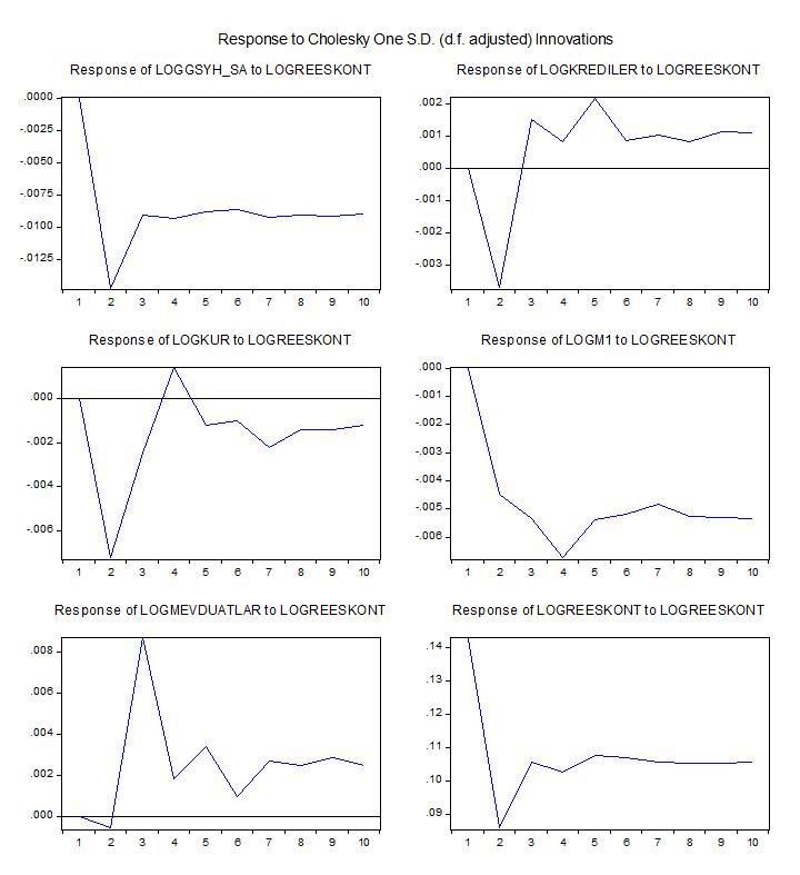
given to the interest rate, it is now discussed how other variables react to a one-unit shock to the exchange rate. In the
same way, the responses of the variables over a period of 10 periods based on the Chelosky method are given in the
following graph and interpreted.
The reaction to the shock given to the exchange rate
in gross domestic product starts with a decrease until
the 2nd period and increases after the 2nd period until
the end of the 3rd period but then decreases again.
The reason for this is the life of GDP, the current
account deficit of Turkey's economy and therefore it
can be interpreted as negative impact of GDP on
exchange rate shock. On the other hand, although
GDP shows an upward trend in some periods, as can
be seen in the graph, it cannot cross the zero line and
continues at a negative level for 10 periods.
Likewise, a negative trend is observed in loans and
this effect below the zero level continues until the 4th
period. Although a positive line is seen from the 4th to
the 7th period, it is seen that after the 7th period it has
a slight negative slope. The impression of this
reaction in credits also indicates that it is compatible
with credit channel theory.
The M1 money supply offers a stronger response to
the exchange rate shock. Following the harsh
negative slope up to the second period, the upward
slope is followed again stiffly. An upward impression
is seen again after a decline until the 6th period.
Moreover, these movements continue above zero
level in M1 money supply.
Figure 4. Results of Impulse-Response Analysis against One Unit of Shock Given to Exchange Rate
Deposits also show a downward movement due to the exchange rate effect, which, as stated in the previous explanations,
suggests that the interest rate policies against exchange rate movements were caused by depreciation in local currency
deposits and caused an upward movement with subsequent interest rate policies. This increase continues until the 5th
period and then recovers with the decline again. On the other hand, the discount interest rate shows a downward decline in
the reaction to the exchange rate shock. These findings, compared to the exchange rate channel of Turkey, show us that
interest rates have more influence on the economy.
5. Results and conclusions
Monetary transmission mechanisms have gained importance in recent years and this shows how accurate and effective
monetary policies are. Monetary transmission mechanisms have been subjected to various but similar classifications in the
literature. However, in this study, our analysis was performed based on the Mishkin classification. The process, through
which Turkey's economy is going recently, increases the importance of this analysis. Turkey is a country that is set to bring
the current account deficit due to problems on the basis of origin. If you want this interest focused on whether the work
42Academic Journal of Economic Studies
Vol. 6 (1), pp. 36–43, © 2020 AJES
done by the exchange rate also results-oriented analysis shows us how and at what level includes an impact for Turkey's
economy. The process in which the Turkish economy has passed in recent periods increases the importance of this
analysis. Since Turkey is a country with a current account deficit, it brings foreign currency problems on the basis of it. This
study shows us how and at what level it has an impact on the Turkish economy, both on interest-oriented and exchange-
rate-oriented analysis results.
In this study, VECM technique was used, since the use of the Vector Error Correction Model would yield more accurate and
healthy results. The quarterly data set covering the periods 2009: 32018: 6 were used for analysis. The data was obtained
from sources, such as Turkey Statistical Institute (TUIK), Turkey Presidency of the Republic of Strategy and Budget
Department and the Central Bank of the Republic of Turkey (CBRT). The variables were divided into two groups as
endogenous and exogenous variables. Internal variables included Gross Domestic Product (GDP), M1 narrow-scale money
supply, discount interest, loans, deposits, and US dollar (USD) and Turkish lira exchange rate. BRENT branded oil prices
per barrel, representing the energy sector, which is an important part of Turkey's current account deficit, were entered as
exogenous variables. The variables used were first subjected to logarithmic transformation, then seasonally adjusted and
then the stationarity test was made by making the series stationary. By measuring the appropriate lag lengths, the number
of observations of the variables was taken into consideration and it was decided to perform the analysis with the lag length
of the first order. No autocorrelation problem was encountered in the study. Then, the variance decomposition test and the
means matrix covering the average of 10 periods were formed for all variables. Then, both the interest rate channel and the
exchange rate channel effect-response analysis were performed and the results were interpreted.
According to the findings, although the effect of the interest rate channel on other variables is simulated in a shorter period
compared to the exchange rate channel, ie it disappears, since the effect on the other variables is longer in the exchange
rate channel, and the exchange rate channel is larger in terms of efficiency, it is obtained that the exchange rate channel is
more effective agent than the interest rate channel for Turkey. The findings reveal that the exchange rate channel is more
important than the interest rate channel for the Turkish economy. Since the exchange rate channel causes deep
fluctuations almost in all variables, it appears that it has potential to move Turkey's economy into a serious crisis.
References
Akbaş, Yusuf, E., Zeren, F., Özekicioğlu, H. (2013). Türkiye’de Parasal Aktarım Mekanizması: Yapısal VAR Analizi, CÜ İktisadi ve İdari
Bilimler Dergisi, Cilt 14, Sayı 2.
Barran, F., Coudert, V., Mojon, B. (1996). The Transmission of Monetary Policy in European Countries, CEPII Document De Travail,
no96-03.
Bernanke, B. S., Blinder, A. S. (1988). Credit Money and Aggregate Demand”, The American Economic Review, Vol. 78, No. 2.
Boughrara, A. (2009). Monetary Transmission Mechanisms in Morocco and Tunusia, Working Paper Series, No. 460, Economic
Research Forum.
Camarero, M., Ordonez, J., Tamarit, C. (2002). Monetary Transmission in Spain: a Structural Cointegrated VAR Approach, Applied
Economics, No.34.
Cengiz, V. (2009). Parasal Aktarım Mekanizması İşleyişi ve Ampirik Bulgular, Erciyes Üniversitesi İktisadi ve İdari Bilimler Fakültesi
Dergisi, Sayı: 33, Temmuz, Aralık 226.
Dovciak, P. (1999). Transmission Mechanism Channels in Monetary Policy, National Bank of Slovakia, Institute of Monetary and
Financial Studies, DOV/ 0008.
Ganev, G., D. (2002). Transmission Mechanism of Monetary Policy in Central and Eastern Europe, Center for Social and Economic
Research, Case Reports no. 52.
Gündüz, L. (2001). Türkiye’de Parasal Aktarım Mekanizması ve Banka Kredi Kanalı, IMKB Dergisi, Sayı.18.
Huseynov, E., Jamilov, R. (2013). Channels of Monetary Transmission in the CIS: a Review, Journal of Economic and Social Studies,
Vol. 3, Nu 1, Spring.
Ireland, P. N. (2006). The Monetary Transmission Mechanism, Boston Colloge Working Paper in Economics.
Mishkin, F. (2004). The Economics of Money, Banking and Financial Markets, Boston: Pearson (The Addison- Wesley series in
economics), 7th edition.
Mojon, B., Peersman, G. (2001). A VAR Description of the Effects of Monetary Policy in the Individual Countries of the Euro Area,
Working Paper Series, No.92, European Central Bank.
Oktar, S., Eroğlu, N., Eroğlu, İ. (2013). Global Finansal Krizi, Parasal Aktarım Kanalları ve Türkiye Cumhuriyet Merkez Bankasının
Deneysel Politika Çalışmaları, Marmara Üniversitesi İİB Dergisi, Cilt XXXV, Sayı 2.
Örnek, İ. (2009). Türkiye’de Parasal Aktarım Mekanizması Kanallarının İşleyişi, Maliye Dergisi, Sayı 156.
Taylor, J. B. (1995). The Monetary Transmission Mechanism: An Empirical Framework, Journal of Economic Perspectives, 9(4), Fall.
Yapraklı, S. (2011). Açık Enflasyon Hedeflemesi Döneminde Parasal Aktarım Mekanizmasının Döviz Kuru Kanalı: Türkiye Üzerine
Ekonometrik Bir Analiz, İstanbul Üniversitesi İktisat Fakültesi Ekonometri ve İstatistik Dergisi, Sayı 15.
43You can also read