The Influence of Relief on the Density of Light-Forest Trees within the Small-Dry-Valley Network of Uplands in the Forest-Steppe Zone of Eastern ...
←
→
Page content transcription
If your browser does not render page correctly, please read the page content below
geosciences
Article
The Influence of Relief on the Density of Light-Forest
Trees within the Small-Dry-Valley Network of
Uplands in the Forest-Steppe Zone of Eastern Europe
Pavel Ukrainskiy 1 , Edgar Terekhin 1 , Artyom Gusarov 2 , Eugenia Zelenskaya 1 and
Fedor Lisetskii 1, *
 1    Federal–Regional Center of Aerospace and Surface Monitoring of the Objects and Natural Resources,
      Belgorod National Research University, 308015 Belgorod, Russia; pa.ukrainski@gmail.com (P.U.);
      terekhin@bsu.edu.ru (E.T.); zelenskaya@bsu.edu.ru (E.Z.)
 2    Institute of Geology and Petroleum Technologies, Kazan Federal University, 18 Kremlyovskaya Str.,
      420008 Kazan, Russia; avgusarov@mail.ru
 *    Correspondence: liset@bsu.edu.ru; Tel.: +7-4722-301370

 Received: 29 August 2020; Accepted: 21 October 2020; Published: 24 October 2020

 Abstract: An active process of the invasion of woody vegetation, resulting in the formation of light
 forests, has been observed in predominantly herbaceous small dry valleys of the forest-steppe uplands
 of the East European Plain over the past two decades. This paper investigates the spatial features of
 the density of trees in such light forests and its relationship with relief parameters. The Belgorod
 Region, one of the administrative regions of European Russia, was chosen as a reference for the
 forest-steppe zone of the plain. The correlation between some relief characteristics (the height, slope,
 slope exposure cosine, topographic position index, morphometric protection index, terrain ruggedness
 index, and width and depth of small dry valleys) and the density of light-forest trees was estimated.
 The assessment was carried out at the local, subregional and regional levels of generalization. The relief
 influence on the density of trees in the small dry valley network is manifested both through the
 differentiation of moisture within the territory under study and the formation of various conditions
 for fixing tree seedlings in the soil. This influence on subregional and regional trends in the density is
 greater than on local trends. The results obtained are important for the management of herbaceous
 small-dry-valley ecosystems within the forest-steppe uplands in Eastern Europe.

 Keywords: trees invasion; trees mapping; smooth interpolation; multiscale patterns; spatial trend;
 geomorphometric features; correlation analysis; Central Russian Upland; Belgorod Region

1. Introduction
     Over the recent 20 years, there has been an active invasion of tree vegetation into the
herbaceous ecosystems in the southwestern part of the European territory of Russia (hereinafter,
European Russia) [1]. This process in the region can be associated both with current climate change [2]
and a decrease in the area of pastures and hayfields due to significant changes in agriculture that
followed after the collapse of the Soviet Union at the end of 1991 [3].
     The expansion of tree vegetation into grasslands was (and is) widely observed in different
regions of the world: in the North American prairies [4–7], South American pampas [8–10], Eurasian
steppes [11], and subalpine meadows of Europe and North America [12–15], and so forth. A specific
feature of the forest-steppe in the southwestern part of European Russia is the dispersal of tree
vegetation along the small dry valley network that has a significant density there and, therefore, has an
impact both on the formation of local landscapes and the features of their economic use.

Geosciences 2020, 10, 420; doi:10.3390/geosciences10110420                   www.mdpi.com/journal/geosciences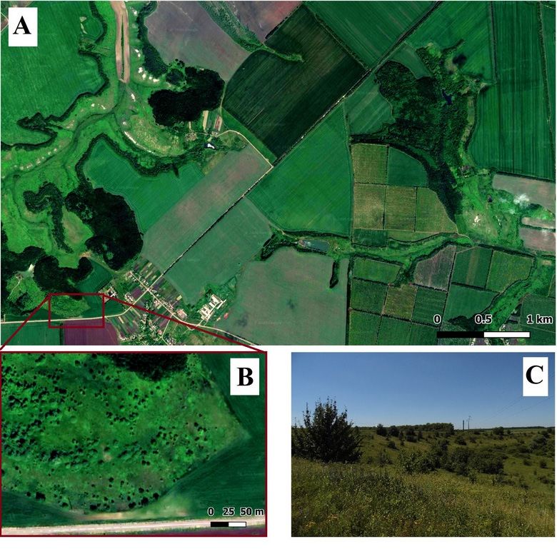
Geosciences 2020, 10, 420 2 of 18
A small dry valley (bálka in Russian terminology) is a dry (or with a temporary snowmelt-induced
or rainfall-induced water stream) valley with soddy slopes. It has a gently concave bottom, often
without a noticeable channel; the slopes are convex, smoothly turning into watersheds. The lengths
of small dry valleys are usually from hundreds of meters to 20–30 km, the depths are from several
meters to tens of meters, and the widths are up to hundreds of meters. The relatively small size and
the absence of a permanent watercourse at the bottom of small dry valleys is one of the diagnostic
features that distinguish them from typical river valleys.
Within this territory, tree vegetation can be resettled from time to time by increasing the area of
artificial windbreaks, as well as the advancement of the boundaries of natural forests [1]. In other cases,
independent light forests are formed in the small dry valley network. They can be both permanent
plant communities and a successional stage in the formation of closed forest communities.
Existing works on the study of the invasion of tree vegetation into herbaceous ecosystems of
Russia mainly concern the distribution of tree (woody) vegetation on abandoned arable lands [16–19].
However, in the southwestern part of European Russia, the spread of abandoned arable land is small
as compared to the rest of the territory, and fallow lands are rare [20–23]. At the same time, the small
dry valley network is widespread there, and it is the main reserve of territories for the resettlement
of tree vegetation — so-called light forests (or open woodlands). The light forests growing in the
network have remained poorly studied up to the present time. This is especially true for their modern
temporal dynamics. Studies in other regions of the world have shown that relief (topography) affects
the tree density in these light forests [24–27] and, therefore, determines many aspects of their ecological
development and economic use.
The aim of the study is to reveal the influence of relief characteristics on the spatial patterns of
changes in the density of trees in light forests in the uplands of the forest-steppe of Eastern Europe.
The implementation of this aim was carried out on the example of the southwestern part of European
Russia within the Belgorod Region. To achieve this aim, the following tasks were solved:
• Collection and systematization of information on tree density in light forests.
• Analysis of changes in the density of trees in light forests in the Belgorod Region.
• Correlation analysis between the relief characteristics of the small dry valley network and the
density of trees in light forests of the region.
• Determination of those relief characteristics that have a predominant influence at different
territorial levels of the study: local, subregional, and regional.
• Interpretation of the revealed patterns.
2. Materials and Methods
2.1. Study Area
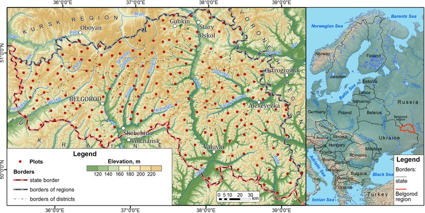
The territory under study is the Belgorod Region. This administrative region of Russia is located
in the southwest of its European part, near the border with Ukraine (Figure 1). The area of the region is
27,100 km2 .
The Belgorod Region is situated in the southern part of the Central Russian Upland, one of the
largest uplands in the East European Plain. The upland’s surface is a hilly plain, dissected by a relatively
dense network of river valleys, small dry valleys, and gullies. The total length of the small dry valleys
network of the region is estimated at 18,500 km, while the total length of the entire erosional network,
including river valleys, is 22,500 km (based on SRTM Void Filled data (version 3.0 with spatial resolution
3 arc second)). The entire erosional network’s density increases from 1.0–1.5 km/km2 in the northwest to
1.8–2.0 km/km2 in the southeast of the region [28]. The general slope of the surface of the region’s territory
is directed to the south. The maximal absolute height is 277.2 m, the minimal is 68.3 m.Geosciences 2020, 10, 420 3 of 18
Geosciences 2020, 10, x FOR PEER REVIEW 3 of 17
Figure Figure
1. The1.territory
The territory under
under study(the
study (theBelgorod
Belgorod Region)
Region) with
withthethe
location of registration
location plots. plots.
of registration
AccordingThe Belgorod
to the Region
Köppen is situated
climate in the southern part [29],
classification of the Central Russian Upland,
the Belgorod Regionone hasof the
a climate
largest uplands in the East European Plain. The upland’s surface is a hilly plain, dissected by a
Dfb—a humid continental climate with warm summers. Air temperatures within the region gradually
relatively dense network of river valleys, small dry valleys, and gullies. The total length of the small
increasedryfromvalleysnorth to south:
network of the the average
region annual
is estimated temperature
at 18,500 km, whilevaries there
the total lengthfrom +6.3
of the
◦ C to +7.5
entire
◦ C, the average January temperature from −6.9 ◦ C to −5.8 ◦ C, respectively (estimates for the period
erosional network, including river valleys, is 22,500 km (based on SRTM Void Filled data (version 3.0
1973–2013withby [30]),resolution
spatial and the 3average July The
arc second)). temperature +19.4 ◦ Cdensity
fromnetwork’s
entire erosional to +20.7 ◦ C [31].
increases from 1.0–1.5
km/km 2 in the northwest to 1.8–2.0 km/km2 in the southeast of the region [28]. The general slope of
Annual precipitation decreases from the northwest to the southeast of the Belgorod Region from
the surface of the region’s territory is directed to the south. The maximal absolute height is 277.2 m,
663 to 614 mm (estimates for the period 1973–2013, according to [32]). Sixty-three percent of the annual
the minimal is 68.3 m.
precipitation occurs during the warm season (the maximum quantity is in June and July). Snow cover
According to the Köppen climate classification [29], the Belgorod Region has a climate Dfb—a
usuallyhumid
forms continental
in December and with
climate meltswarmin March.
summers. Its depth at the end within
Air temperatures of winterthe is mostgradually
region often 20–30 cm.
The duration
increaseoffrom thenorth
snowtocoversouth: is
the100–120 days [31,33].
average annual temperature varies there from +6.3 °C to +7.5 °C, the
Theaverage
BelgorodJanuary temperature
Region belongs frompredominantly
−6.9 °C to −5.8 °C, to respectively (estimates for
the forest-steppe the period
zone of the1973–2013
East European
by [30]) , and the average July temperature from +19.4 °C to +20.7 °C
Plain. Before the start of economic development, the steppes growing on chernozem soils occupied [31].
Annual precipitation decreases from the northwest to the southeast of the Belgorod Region from
most of its territory. The steppes were interspersed with oak forest patches growing on gray forest
663 to 614 mm (estimates for the period 1973–2013, according to [32]). Sixty-three percent of the
soils. Acer
annualplatanoides
precipitationL., Tilia
occurs cordata
duringMill., Fraxinus
the warm seasonexcelsior L., andquantity
(the maximum elms also is incurrently grow in oak
June and July).
forests, Snow
alongcover Quercus
withusually robur
forms in December and melts in March. Its depth at the end of winter is mostBy now,
L. Pine forests grew (and grow) on sandy riverine terraces.
almost all steppes that were widespread
often 20–30 cm. The duration of the snowthere in the
cover 17th century
is 100–120 days [31,have33]. been ploughed up. In addition,
The Belgorod Region belongs predominantly
by now, two-thirds of the forests that grew there in the 17th century have to the forest-steppe zone
been of cut
the East
down,European
and then soils
Plain. Before the start of economic development, the steppes growing on chernozem soils occupied
beneath them have also been ploughed up [34]. The ecological specificity of forests in the forest-steppe
most of its territory. The steppes were interspersed with oak forest patches growing on gray forest
and steppe environments is well-diagnosed by differences in the rate of pedogenesis [35]. By now,
soils. Acer platanoides L., Tilia cordata Mill., Fraxinus excelsior L., and elms also currently grow in oak
cultivated lands
forests, along occupy about 60%
with Quercus roburofL. the
Pineregion’s
forests grewterritory, while
(and grow) onabout 12% of terraces.
sandy riverine its area By
is still
now,forested.
Pastures almost all steppes that were widespread there in the 17th century have been ploughed up. In addition, in the
and hayfields, which occupy 17% of the region’s territory, are concentrated mainly
small dryby now,
valleys two-thirds
network, of the forestsasthat
as well grew there
in river in the 17th century have been cut down, and then
valleys.
Thesoils beneath
object them
of the have also
study been the
(within ploughed
Belgorod up [34]. The ecological
Region) specificity
is the small dry of forests network
valleys in the forest-
prevailed
steppe and steppe environments is well-diagnosed by differences in the rate of pedogenesis [35]. By
by herbaceous steppe vegetation [36]. However, small-sized wooded areas can be also located in the
now, cultivated lands occupy about 60% of the region’s territory, while about 12% of its area is still
upper parts of Pastures
forested. the network. The economic
and hayfields, which occupy use17%of small dry valleys
of the region’s in the
territory, region is represented
are concentrated mainly by
haymaking and grazing [3]. The network is usually
in the small dry valleys network, as well as in river valleys. surrounded by croplands. In many cases, small
dry valley systems
The objectare fringed
of the by (woody)
study (within windbreaks,
the Belgorod Region) ismost of which
the small werenetwork
dry valleys created by humans in
prevailed
the 1960sby [37].
herbaceous
Thus,steppe vegetation
artificial [36]. However,
windbreaks are often small-sized
locatedwooded areas can
at the border ofbecroplands
also locatedandin the
small dry
valleys.upper parts of light
At present, the network.
forestsThe areeconomic
widespread use ofthroughout
small dry valleys in thedry
the small region is represented
valleys network. byIn most
cases, these are plots with an area of up to several tens of hectares. The species composition of the
light forests in the Central Russian Upland basically includes wild fruit trees and shrubs—apple trees,
pear trees, hawthorn, and wild rose [38]. From time to time, some forest species can penetrate into
the light forests from the nearby indigenous forests and artificial windbreaks. Normally, there are
elms, Acer platanoides L. and Acer tataricum L., Fraxinus excelsior L., and, occasionally, Quercus robur L.Geosciences 2020, 10, 420 4 of 18
in the light forests. Some alien species (Robinia pseudoacacia L. and Acer negundo L.) are also actively
introduced into the light forests [39,40].
2.2. Source Materials
The light forests growing in the small dry valleys network of the Belgorod Region were
studied using ultra-high spatial resolution satellite images. We used mosaics of space images
provided by web mapping services, primarily by Google Earth. The images were analyzed using the
QGIS 3.10 software [41]. The plugin QuickMapServices was used.
The sections of the small dry valleys network with growing light forests were selected by a visual
analysis of remote-sensing data. All areas with forest vegetation, the crowns of which do not close
together, are categorized as light forests. That is, free-standing trees are clearly visible against the
background of grass. A rectangular area of 1 hectare was allocated on these territories. The plots were
prepared in a vector layer with polygonal geometry. The sides’ sizes of the plot were 100 × 100 m or
50 × 200 m, depending on the shape and size of a particular section of the small dry valleys network.
A total of 200 plots were identified (see Figure 1). The location of the plots was predetermined by the
structure of the small dry valleys network and the presence of light forests in it. The light forests do not
have continuous distribution in the small dry valleys network. They are found as separate fragments.
The plots are confined to these fragments.
To select the plots (sites), light forests were selected in such a way that the uniformity of their
distribution over the territory of the Belgorod Region was ensured. The Clark-Evans test [42] was
used to meet this requirement. The test was performed in the R statistical environment using the
spatstat add-on package [43,44]. The test variant with boundary correction was also used. According
to the test results, the value of the Clark-Evans test R was 1.44 (p = 0.002). This indicated a statistically
significant deviation of the area distribution from the random spatial distribution. Since the criterion
value was greater than 1.0, the distribution was uniform (for values less than 1.0, this would be the
group distribution).
The light forest areas, in which 200 sites (plots) were established, have an area of 2 to 63 hectares
(on average, 11 hectares). The distance between the nearest sites ranged from 4.0 to 17.4 km (on average,
8.9 km; the standard deviation was 2.5 km).
All trees within each plot were manually vectorized in a point feature layer (Figure 2). Individual
trees were identified using mosaics of images with ultra-high spatial resolution (more detailed 1 m/pixel).
That is, the size of the crowns of individual trees was always somewhat larger than the pixel size
of the mosaic images. All satellite data used were obtained during the active growing season. Due
to the relatively small area of the region studied, the phenological phases differed insignificantly
within its limits. Due to taking into account the listed criteria, the obtained experimental data can be
considered objective.
After vectorization, the density of trees was calculated for each plot and entered into the attribute
table of the polygonal layer of the plots. The study of the density of trees in the regional light forests
was carried out without differentiating them by species composition.Geosciences 2020, 10, 420 5 of 18
Geosciences 2020, 10, x FOR PEER REVIEW 5 of 17
2. An
Figure 2.
Figure Anexample
exampleofoflight forests
light in satellite
forests images
in satellite and on
images andtheonground: (A) Small
the ground: (A) dry valley
Small drygeneral
valley
general view with a light forests. (B) Small dry valley fragment with a light forest. (C) Light ground
view with a light forests. (B) Small dry valley fragment with a light forest. (C) Light forest’s forest’s
photography
ground (typical (typical
photography light forest near
light thenear
forest villagetheofvillage
L’vovka, east of the
of L’vovka, Belgorod
east Region). Region).
of the Belgorod
The following
The following groupgroup of
of variables
variables was
was studied
studied toto estimate
estimate thethe relief’s
relief’s effect
effect on
on the
the density
density of
of trees
trees
in light
in light forests:
forests: thethe absolute
absolute height,
height, slope,
slope,aspect,
aspect,topographic
topographicposition
positionindex
index(TPI),
(TPI),profile
profilecurvature,
curvature,
morphometric protection index (MPI), terrain ruggedness index (TRI),
morphometric protection index (MPI), terrain ruggedness index (TRI), and width and depth of and width and depth of small
small
dry valleys (see Table 1). When analyzing the relief’s characteristics, we used
dry valleys (see Table 1). When analyzing the relief’s characteristics, we used a digital elevation a digital elevation model
(DEM) (DEM)
model with a spatial
with a resolution of 30 m/pixel
spatial resolution of 30 [45]. This[45].
m/pixel DEM wasDEM
This used was
to construct
used to raster models
construct of
raster
the derived relief’s characteristics. Relief characteristic values (except for the
models of the derived relief’s characteristics. Relief characteristic values (except for the width andwidth and depth of the
small dry
depth valleys)
of the smallwere ArcGIS-computed
dry valleys) for each studyfor
were ArcGIS-computed plot. Forstudy
each this, aplot.
zonal
Forstatistics tool was
this, a zonal used;
statistics
that is, an average value was calculated for all pixels within the plot.
tool was used; that is, an average value was calculated for all pixels within the plot.
Besides the relief characteristics, this paper analyzed the nontopographic features (see Table 1),
which can demonstrate
Table 1. Analyzedthe impact
factors produced
affecting by the
the density of climate, the forests.
trees in light practical usedigital
DEM: of a small dry valleys,
elevation
and the location
model, MPI: morphometric protection index, and TRI: terrain ruggedness index [3,45–54]. of light
of tree seed import sources. The significance of the relief for the development
forests in the small dry valley network can be described in more detail by comparing correlations with
Source of Initial Software for
relief-related tree density
Characteristics Units
and nontopographic
Data for
features.
Initial Data Development Description
Development Processing
Relief characteristics
Absolute
m ArcGIS Ready-made DEM was used
height
Slope raster were acquired in ArcGIS 10.5 using
Slope degree ArcGIS
standard Spatial Analyst tools.
The slope exposure (aspect) was converted to
DEM from the
cosine for further use in statistical analysis. The
paper by Buryak
analysis methods we used are designed to work
et al., 2019 [45]
with continuous data, while the aspect is circular
Aspect - ArcGIS
data. Cosine transform allows creating the
continuous data from circular data [46]. To do
this, first an aspect raster with values in degrees
was created in ArcGIS 10.5 software. Then, theGeosciences 2020, 10, 420 6 of 18
Table 1. Analyzed factors affecting the density of trees in light forests. DEM: digital elevation model, MPI: morphometric protection index, and TRI: terrain ruggedness
index [3,45–54].
Source of Initial Data for Software for Initial Data
Characteristics Units Development Description
Development Processing
Relief characteristics
Absolute height m ArcGIS Ready-made DEM was used
Slope raster were acquired in ArcGIS 10.5 using standard Spatial Analyst
Slope degree ArcGIS
tools.
The slope exposure (aspect) was converted to cosine for further use in
statistical analysis. The analysis methods we used are designed to work
with continuous data, while the aspect is circular data. Cosine transform
allows creating the continuous data from circular data [46]. To do this,
first an aspect raster with values in degrees was created in ArcGIS 10.5
Aspect - ArcGIS
software. Then, the aspect values were converted into radians using the
Map Algebra tool, and the cosine of these values was calculated.
The aspect cosine ranges from 1.0 for north to −1.0 for south. It shows
how much the real value of the aspect differs from the north aspect.
Therefore, the aspect cosine is called “northness” [47].
The topographic position index (TPI) indicates which part of the slope a
point is located in [48]. Positive index values indicate a position above
the midpoint of the slope, negative values below the midpoint of the
ArcGIS and Land Facet Corridor slope. The TPI is calculated as the difference between the height of a
TPI -
[49] point and the average height in a certain search radius [50]. A search
radius of 1000 m was used to calculate the TPI. The TPI was calculated in
a standardized way; that is, it divided by the standard deviation of
DEM from the paper by Buryak et heights in the search radius.
al., 2019 [45]
Profile curvature raster were acquired in ArcGIS 10.5 using standard
Profile curvature m−1
spatial analyst tools.
The algorithm analyzes the immediate surroundings of each DEM pixel
in a given search radius and estimates how much the relief protects this
MPI - SAGA [51] point from the surrounding terrain. This is equivalent to positive
openness [52]. The MPI was also calculated with a search radius of 1000
m.
TRI shows how large a difference in elevation is observed at a particular
point in the terrain. It was calculated by determining the difference in
heights between a specific DEM pixel and its eight immediate neighbors
TRI - SAGA [51]
(the calculation was carried out in a sliding window of 3 × 3 pixels).
Then the mean of these differences squares was calculated. The square
root of this mean is the TRI [53].Geosciences 2020, 10, 420 7 of 18
Table 1. Cont.
Source of Initial Data for Software for Initial Data
Characteristics Units Development Description
Development Processing
The small dry valley width was measured directly at those locations of
the sites where the trees were vectorized. For this, a linear layer was
created in which lines were drawn across small dry valleys: the lines
were drawn from edge to edge, crossing the site. The small dry valley
Width of small dry valleys m Mosaics of space images from ESRI ArcGIS widths were calculated as the lengths of these lines. The geometry
World Imagery calculation tool in the layer’s attribute table was used for this. The small
dry valley depths were measured as the difference between the minimal
(along the thalweg line) and maximal heights within this line. For this
purpose, such an indicator of zonal statistics as range of values was
Depth of small dry valleys m ArcGIS extracted from the DEM along the line using ArcGIS 10.5 software.
Non-topographic features
A raster was interpolated along the contour lines plotted by the authors.
Hydrothermal index (HTI) - Lebedeva et al., 2019 [54] ArcGIS
Zonal statistical values extracted from the raster.
The layer of forests (authors data)
A distance to the nearest
km The layer of windbreaks ArcGIS The nearest object standard tool used.
windbreaks or forest
(authors data)
The area of the nearest forest ha The layer of forests (authors data) ArcGIS The nearest object standard tool used.
The layer of windbreaks The density of windbreaks was calculated for the Thiessen polygons
Density of windbreaks km/km2 ArcGIS
(authors data) constructed around the sites
Share of unused pastures and
Values to be taken from WMS available layer
hayfields split by % Kitov, 2015 [3] ArcGIS
https://qgiscloud.com/deppriroda/cons/wms
municipalitiesGeosciences 2020, 10, 420 8 of 18
2.3. Research Methods
We performed all statistical data analyses in the statistical computing environment R 3.4.4 [43].
Smoothing interpolation was used to create tree density change maps for the light forest located in
the territory of the Belgorod Region. The interpolation was performed in the R statistical computing
environment with the use of the optional spatstat package [44]. The Smooth function of this package
implements a smoothing interpolation. It is based on the calculation of the locally weighted average
using the Nadaraya-Watson formula [55,56]. The kernel type and the presence of boundary correction
are the key settings for the interpolation process performed by the Smooth search radius function.
We used a Gaussian kernel and boundary correction, as previously suggested by Diggle [57]. Using this
interpolation, we could obtain several rasters created with different search radii (5, 10, 15, 20, 25, 30,
35, 40, 45, and 50 km). With the search radius being increased, the generalization of the resulting
maps can be improved. This makes it possible to identify trends in tree density at different scale
levels. This approach is based on the concept of the poly-scale organization of landscapes [58–62].
We considered three large-scale levels: local, subregional, and regional. In our case, the regional
level covers the territory of the entire Belgorod Region. It corresponds to search radii of 40–50 km.
The subregional level covers individual physical geographic districts of the region and their parts.
It corresponds to search radii of 15–25 km. The local level is reduced to individual local landscapes
within the physical geographic districts of the region. It corresponds to a search radius of 5 km.
The Smooth function can return not only a bitmap but, also, local mean values at the original points.
For each search radius, we calculated the local average density of trees in light forests. The obtained
values were used in the correlation analysis.
The correlation between the density of trees in light forests and the above relief’s variables has
been estimated in the study. Initial density values and local mean values obtained from ten different
search radii were used to calculate the correlation. The correlation between various variables of the
relief was also calculated. Using the cor.test function, Spearman’s correlation coefficients were also
calculated. The Spearman’s Rank correlation coefficient [63] was used due to the fact that the analyzed
indicators have a distribution that differs from the normal one. The normality of the distribution was
assessed with the Shapiro-Wilk test [64] (the R function shapiro.test).
3. Results and Discussion
3.1. Changes in the Density of Trees in Light Forests of the Belgorod Region
Table 2 shows the estimated tree densities obtained for different search radius values in the
smoothing interpolation. A zero search radius means the initial raw data—the number of trees counted
on the sites.
The resulting maps of the density of trees in light forests for the local, subregional, and regional
levels are shown in Figure 3. A variegated pattern of changes in the density of trees in light forests is
observed at the local level, since there are high and low values of this density in any part of the Belgorod
Region. At the same time, the transition from high values to low ones in the most cases occurs at a
distance of only 25–30 km. Areas with high and low tree density values at the local level include three
to ten sites. There are some areas, representing high-spatial and low-spatial outliers. High outliers are
sites with high tree density values, all neighbors of which have low values. Low outliers are areas with
low tree density values, all neighbors of which have high values.Geosciences 2020, 10, x FOR PEER REVIEW 8 of 17
Table 2. The density of trees (pcs. per ha) in light forests, estimated for various search radii of the
smoothing interpolation.
Search
Geosciences 2020, Radius, km
10, 420 Minimum Mean Median Maximum Standard Deviation 9 of 18
0 21.00 111.15 99.00 415.00 62.70
5 40.20 115.19 106.86 370.51 46.74
Table 2. The density of trees (pcs. per ha) in light forests, estimated for various search radii of the
10 49.82 112.33 107.49 206.02 26.53
smoothing interpolation.
15 61.23 112.46 107.29 165.75 19.93
Search Radius, km20 Minimum 75.81 112.78
Mean 108.31
Median 154.28
Maximum 16.28
Standard Deviation
25 82.80 112.92 110.57 146.11 13.37
0 21.00 111.15 99.00 415.00 62.70
30 88.77 112.99 113.09 138.10 10.97
5 35 40.20 93.89 115.19 113.01 113.08 106.86 130.99 370.51 9.05 46.74
10 40 49.82 97.30 112.33 112.00 113.07 107.49 127.50 206.02 7.56 26.53
15 45 61.23 99.06 112.46 112.95 112.82 107.29 125.65 165.75 6.41 19.93
50 100.56 112.88 112.96 123.92 5.53
20 75.81 112.78 108.31 154.28 16.28
25 resulting maps82.80
The of the density112.92
of trees in light110.57 146.11subregional, and
forests for the local, 13.37
regional
levels30
are shown in Figure 3. A variegated
88.77 112.99pattern of changes
113.09 in the density
138.10 of trees in light forests is
10.97
observed
35 at the local level,
93.89 since there are high and 113.08
113.01 low values of this density in any part
130.99 9.05of the
Belgorod Region. At the same time, the transition from high values to low ones in the most cases
occurs40at a distance of only
97.3025–30 km. 112.00
Areas with high113.07 127.50 values at the local
and low tree density 7.56 level
45 three to ten sites.
include 99.06 112.95
There are some 112.82 high-spatial
areas, representing 125.65 and low-spatial6.41outliers.
High 50
outliers are sites 100.56
with high tree 112.88
density values, 112.96
all neighbors of123.92
which have low values.5.53 Low
outliers are areas with low tree density values, all neighbors of which have high values.
Figure
Figure 3. The
3. The densityof
density of trees
trees in
inlight
lightforests at at
forests thethe
local ((A),((A),
local search radiusradius
search 5 km), 5subregional ((B),
km), subregional
search radius 15 km), and regional ((C), search radius 50 km) scale levels of generalization within the
((B), search radius 15 km), and regional ((C), search radius 50 km) scale levels of generalization within
Belgorod Region, SW Russia.
the Belgorod Region, SW Russia.
In contrast to the local level, you can notice clearly expressed territorial patterns at the subregional
level. From west to east, there is an alternation of areas with an increased and decreased density
of trees. However, spatial outliers of high or low values at the subregional level are not detected.
The reasons for the formation of such a tree density geography in the light forests at the subregional
level need to be studied additionally within the framework of separate research. We assume that,
for the two areas with the highest values of the density of trees, the leading formation factors areGeosciences 2020, 10, 420 10 of 18
different. The formation of such an area around the city of Belgorod is associated with the low intensity
of the economic use of the small dry valleys network there. According to existing estimates, more
than 75% of natural forage lands are not used around the city [3]. The lack of grazing and haymaking
creates favorable conditions for the settlement of forest vegetation in the small dry valleys network.
In the area of high tree density along the Valuyki-to-Alexeyevka line (see Figure 3), the share
of unused natural forage lands is also increased, although to a lesser extent than around the city
of Belgorod. There, the share of unused natural grasslands reaches 70–90% and, in the vicinity of
Belgorod, it is 85–95% [3]. However, this factor is reinforced by the presence of powerful sources for
the import of seeds of forest plants: to the north of the towns of Valuyki and Alexeyevka (see Figure 3),
there are wooded areas that are one of the largest forestlands in the Belgorod Region. Many small
dry valleys are located next to them, and some of the valleys begin right in the forestlands. Areas of
increased density of trees in light forests (more than 100 trees per hectare) mainly cover the middle and
lower parts of the basins of large rivers of the Belgorod Region. There are three such areas in total
in the region. The western area is the lower part of the Vorskla River basin, as well as the basins of
the Vorsklitsa River and Ilek River. This area includes 16 plots. The density there is 100–110 trees per
hectare. The central area is the lower parts of the basins of the Seversky Donets River and Nezhegol
River. This area includes 41 plots. The density there is 100–180 trees per hectare. The eastern area is
the basins of the Tikhaya Sosna River and Userdets River (see Figure 3A). This area includes 66 plots.
The density there is 100–145 trees per hectare.
Areas of low tree density in light forests (less than 100 trees per hectare) at the subregional level are
confined to the largest river’s interfluves, as well as to the upper parts of their basins. There are three
such sites in the region. The largest of them is situated in the center of the Belgorod Region and covers
the interfluve of the Seversky Donets River and Oskol River, as well as the upper parts of the basins of
the Oskol, Seym, Nezhegol, Koren, and Korocha Rivers (see Figure 3B). This area includes 42 plots.
A decrease in the density of trees in light forests is observed there from south to north. In this direction,
the density decreases from 110 to 80 trees per hectare. Two more areas of low tree density in light
forests are located in the southeastern (the Aidar River basin) and the northwestern (the interfluves of
the Vorskla River, Psel River, and Pena River) parts of the Belgorod Region (see Figure 3B). The first
area includes nine plots and the second one, 23 plots. In the southeastern area, the density in open
woodlands is 90–100 trees per hectare and, in the northwestern area, 80–90 trees per hectare.
At the regional level, there is no alternation of areas of high and low density of trees. Instead,
there is a unidirectional increase in tree density in the open woodlands from 100–102 to 118–124 trees
per hectare. This increase occurs in the direction from northwest to southeast. Its maximal values are
reached in the interfluve area of the Tikhaya Sosna, Oskol, and Aidar Rivers (see Figure 3C). As well as
at the subregional level, there are no spatial outliers of high or low values of the density of trees in
light forests at the regional level of the study.
The absolute height of the base surfaces (that is, the height of small dry valley bottoms) decreases
from the northwest to the southeast of the Belgorod Region (from 170–200 m to 90–120 m), and the
vertical dissection of the topographic surface increases from 30–40 m to 70–80 m, respectively [28].
At the same time, the availability of groundwater for forest vegetation increases in small dry valleys.
As stated earlier, from the northwest to the southeast of the Belgorod Region, air temperatures also
increase, while the annual precipitation decreases [28]. These circumstances impede the spread of forest
vegetation in the indicated direction. The geography of the density of trees observed at the regional
level shows that favorable geomorphic conditions in the small dry valleys network compensates for
the unfavorable climatic conditions there. For the forest-steppe and steppe zones, this was noted
earlier, but on the example of the existence of small-dry-valley dense forests (bairak forests in Russian
terminology—forests that grow in small areas on the tops and slopes of small dry valleys in the steppe
and forest-steppe zones) [65]. In our study, we observed a new form of this regularity manifestation by
the example of light forests.Geosciences 2020, 10, x FOR PEER REVIEW 10 of 17
compensates for the unfavorable climatic conditions there. For the forest-steppe and steppe zones,
this was noted earlier, but on the example of the existence of small-dry-valley dense forests (bairak
Geosciences 2020,
forests 10, 420 terminology—forests that grow in small areas on the tops and slopes of small dry11 of 18
in Russian
valleys in the steppe and forest-steppe zones) [65]. In our study, we observed a new form of this
regularity manifestation by the example of light forests.
3.2. Correlation of Tree Density and Relief Characteristics
3.2.
TheCorrelation
values of ofthe
Tree Density
local and Relief
average Characteristics
density of trees obtained with different search radii have different
strengthsTheof relationships with
values of the local the relief
average (Figure
density of trees4). According
obtained to this search
with different connection’s form,
radii have the relief
different
strengths of relationships with the relief (Figure 4). According to this connection’s form,
characteristics can be divided into three groups. The first group is those variables that have a negative the relief
characteristics
correlation with thecandensity
be dividedof into
treesthree groups.height
(absolute The first group
and theistopographic
those variables that have
position a negative
index). With an
correlation with the density of trees (absolute height and the topographic position index). With an
increase in the search radius, the strength of a relationship for these variables increases. The second
increase in the search radius, the strength of a relationship for these variables increases. The second
group consists of those variables that have a positive correlation with the density of trees (the aspect
group consists of those variables that have a positive correlation with the density of trees (the aspect
“northness”, width, and depth of small dry valleys). With an increase in the search radius, the strength
“northness”, width, and depth of small dry valleys). With an increase in the search radius, the
of a relationship between these
strength of a relationship variables
between these also increases.
variables also increases.
Figure 4. Changes
Figure in in
4. Changes thethe
correlation
correlationcoefficient betweenthe
coefficient between thedensity
density of trees
of trees andand the studied
the studied relief relief
characteristics with
characteristics anan
with increase
increaseininthe
thesearch
search radius withthe
radius with thesmoothing
smoothing interpolation
interpolation (statistically
(statistically
significant (pThe third group includes the relief characteristics that also show a positive correlation with the
tree density (the morphometric protection index (MPI), terrain ruggedness index (TRI), profile
curvature, and aspect). However, with search radius being increased, the relationship strength first
increases (up to a search radius of 25 km) and then decreases. This can be due to complication of the
Geosciences 2020, 10, 420 12 of 18
interrelationships between factors because of the transition to another hierarchical level of the
landscape structure.
At the local level, the lowest correlation between the relief and the density of the trees can be
the Spearman’s correlation coefficients are statistically insignificant for search radii up to five km.
observed. For all relief characteristics studied, except for the slope and terrain ruggedness index
Based on this, it can be assumed that, at the local scale level, the relief is not the leading factor in
(TRI), the Spearman’s correlation coefficients are statistically insignificant for search radii up to five
the formation
km. Based of on light
this, itforests in small that,
can be assumed dry valleys of the
at the local scaleregion. The
level, the location
relief of tree
is not the thefactor
leading seed in
import
sources [39,40] and the nature of the economic use (grazing and haymaking, as well
the formation of light forests in small dry valleys of the region. The location of tree the seed import as grass burning)
of thesources
small dry valleys
[39,40] and the network [3]the
nature of caneconomic
be of great
use importance
(grazing andin the local level.
haymaking, as wellHowever, this requires
as grass burning)
separate
of theresearch.
small dry valleys network [3] can be of great importance in the local level. However, this
requires
For fourseparate research. relief characteristics (the aspect, morphometric protection index MPI,
of the considered
For four of
terrain ruggedness index the considered
TRI, and relief characteristics
profile curvature), (the aspect,
the morphometric
maximal correlation protection
with theindex MPI,of the
density
terrain ruggedness index TRI, and profile curvature), the maximal correlation
trees is achieved at a search radius of 25 km. The same can be said about the depths of small with the density of the dry
trees is achieved at a search radius of 25 km. The same can be said about the depths of small dry
valleys. Although it shows a growing correlation at search radii of more than 25 km, this growth is
valleys. Although it shows a growing correlation at search radii of more than 25 km, this growth is
already insignificant. Thus, the slope, MPI, TRI, profile curvature, and the depths of small dry valleys
already insignificant. Thus, the slope, MPI, TRI, profile curvature, and the depths of small dry valleys
havehave
the greatest influence
the greatest influenceononthe
thedensity
densityofof the treesatatthe
the trees thesubregional
subregional level
level of study.
of the the study. The shapes
The shapes
of theofcorrelation fields for a search radius of 25 km are depicted in
the correlation fields for a search radius of 25 km are depicted in Figure 5. Figure 5.
Figure 5. The
Figure relationship
5. The between
relationship betweenthe
thestudied reliefcharacteristics
studied relief characteristics and
and thethe density
density of trees
of trees in light
in light
forests withwith
forests a search radius
a search ofof
radius 2525km
kmininaasmoothing interpolation.
smoothing interpolation.
For the additional four relief characteristics (the slope, north aspect, TPI, and small dry valley
width), the maximal correlation with the density of the trees can be achieved with a search radius of
50 km. The influence of these characteristics prevails at the regional level.
Table 3 demonstrates the intercorrelation of the relief characteristics. The obtained correlation
matrix shows that it is potentially possible to abandon the use of the TRI, since it has a correlation with
the slope factor of 0.99. The rest of the indicators are less related to each other (absolute values of the
correlation coefficients are not more than 0.75), but each is of interest separately.Geosciences 2020, 10, 420 13 of 18
Table 3. Correlation matrix for the relief variables studied.
Small Dry Small Dry
Relief Variables Height Slope Northness TPI TRI MPI Profile Curvature
Valley Width Valley Depth
Height 1.00 −0.22 −0.28 0.47 −0.21 −0.29 −0.23 −0.38 −0.21
Slope −0.22 1.00 0.27 −0.03 0.35 0.55 0.99 0.46 −0.22
Northness −0.28 0.27 1.00 −0.19 0.25 0.29 0.27 0.18 0.06
TPI 0.47 −0.03 −0.19 1.00 −0.08 −0.21 −0.05 −0.62 −0.60
Small dry valley width −0.21 0.35 0.25 −0.08 1.00 0.75 0.33 0.21 −0.21
Small dry valley depth −0.29 0.55 0.29 −0.21 0.75 1.00 0.55 0.42 −0.11
TRI −0.23 0.99 0.27 −0.05 0.33 0.55 1.00 0.51 −0.18
MPI −0.38 0.46 0.18 −0.62 0.21 0.42 0.51 1.00 0.60
Profile curvature −0.21 −0.22 0.06 −0.60 −0.21 −0.11 −0.18 0.60 1.00
NB: The statistically significant (p < 0.05) correlation coefficients are highlighted in bold.Geosciences 2020, 10, 420 14 of 18
As regards the insufficient humidification in the Belgorod Region (especially in its southern and
southeastern parts), the humidification degree is the main limiting factor for the development of forest
vegetation. The diversity of small dry valley network topography leads to a variety of microclimates
and determines the variations of moisture conditions. The closer the aspect (slope exposure) is to the
northern direction, the better the conditions for humidification of slope landscapes, primarily due
to the lower insolation heating [66]. In the warm season, less moisture evaporates on such slopes.
This pattern is especially noticeable in the temperate latitudes of Earth. In addition, on north-oriented
slopes, the snow lingers longer in the spring, and its melting occurs relatively slower [67]. Slopes with
a concave profile provide a concentration of surface water runoff, while slopes with a convex profile
disperse the runoff. Therefore, the lower the value of the profile curvature, the better, with other things
being equal, such as the moistening of the soil [68]. Consequently, more favorable conditions for tree
growth are formed.
In the Belgorod Region, it is the absolute height and the related relief characteristics (the topographic
position index and small dry valley depth) that determine the distance from the ground surface to
the nearest aquifer, which also feeds tree roots with water and substances dissolved in it. Therefore,
the lower a plot is located from a geomorphological point of view, the better, other things being equal
for the conditions for tree growth there.
The slope and TRI are related to ground surface erosional features. The larger these variables,
the more small-dry-valley slopes are eroded, other things being equal. With increasing the slope
and TRI, the number of gullies (including side gullies) increases. The erosional microrelief helps
the trees to be fixed, since the existing areas of bare soil/ground allow tree seedlings not to compete
with grassy vegetation. Moreover, the increased snow accumulation, usually observed in gullies and
small side hollows, increases the moisture content of the soil and ground in the spring (snowmelt)
season [67]. In addition, areas with steep slopes and an abundance of gullies are of little use for farming.
Haymaking and cattle grazing are also difficult within them.
3.3. The Impact Produced by Nontopographic Factors on Tree Density in Light Forests
In addition to the relief, the location of tree seed import sources can produce an impact on the
density of trees in light forests. At the local level, you can observe a significant correlation related
with the distance from potential sources of forest species introduction (distance to the nearest forest or
windbreaks)—Spearman’s ρ = −0.18 at p = 0.01. Additionally, the density of the trees correlates with
the nearest forest area (for σ = 0, Spearman’s ρ = 0.21 at p = 0.003). At the subregional level, there is a
significant correlation with windbreak density in the immediate vicinity of a plot (Spearman’s ρ = 0.20
at p = 0.004).
However, we failed to find a correlation with the hydrothermal index [54], which would have a
biological meaning. We expected that the higher the hydrothermal index, the higher the density of
trees in light forests. However, the hydrothermal index showed a negative tree density correlation
(at the local level: Spearman’s ρ = −0.23 at p = 0.001, at the subregional level: Spearman’s ρ = −0.36
at p = 1.17 × 10⁻⁷ , and at the regional level: Spearman’s ρ = −0.89 at p < 2.2 × 10⁻¹⁶ ). In this case,
we have a correlation in place, but obviously, there is no causation. Moreover, the hydrothermal
index can well-correlate with the absolute height factor (Spearman’s correlation coefficient ρ = 0.60 at
p < 2.2 × 10⁻¹⁶ ). Thus, the climate effect is interrupted by the impact produced by the relief.
The anthropogenic load on pastures and hayfields tends to have an impact on the density of trees
in light forests. The greater the proportion of unused natural forage lands, the higher the density of
trees. For the local level: Spearman’s ρ = 0.22 at p = 0.002, at the subregional level: Spearman’s ρ = 0.38
at p = 3.05 × 10⁻⁸ , and at the regional level: Spearman’s ρ = 0.24 at p = 0.001.
When comparing the tree density correlation with relief and nontopographic factors, we found
that they are close values. In terms of their impact, the nontopographic factors can only exceed the
relief at the local level. At the subregional and regional levels, they are weaker than the relief impactGeosciences 2020, 10, 420 15 of 18
(for tree seed import source location) or equal to the relief influence (as regards the anthropogenic load
on pastures and hayfields).
4. Conclusions
By the example of the Belgorod Region, for the first time for the landscapes of the forest-steppe
uplands typical of the East European Plain, the main regularities of contemporary changes in the
density of trees in light forests of the network of small dry valleys were revealed. The emergence of
these light forests is the latest trend in the development of vegetation cover in the region.
The geographic features of these changes at various scale levels of the study (generalization)
are very different. At the local level, a variegated spatial spreading is observed in which there are
no obvious spatial patterns in changes in the tree density. More or less noticeable patterns begin to
be determined with an increase in the generalization of tree density cartograms. At the subregional
level, there is an alternation of areas with high and low densities of trees from the west to the east
of the Belgorod Region. The areas of increased density mainly covered the middle and lower parts
of the basins of the large rivers there, while the areas of low density of the trees in light forests at
the subregional level are confined to the interfluves of the largest rivers of the region, as well as to
the upper parts of their basins. The region-wide (that is, the most generalized) trend is a consistent
increase in the density of light-forest trees in the small dry valleys network from the northwest to the
southeast of this administrative region of SW European Russia.
Relief characteristics also affect the density of the trees in light forests growing in the small dry
valleys network. Their influence is manifested through the differentiation of the moisture conditions in
the territory studied and the creation of various conditions for the fixing of tree seedlings in the soil.
At the local level, the relief influence is minimal, and the density of trees is largely due to other factors.
Of all the relief characteristics at the local level, statistically significant correlation was found only
for the slope and TRI. In general, at the subregional and regional levels of generalization, the closest
correlation is observed with the absolute height of a particular territory. The second most important
factor at the subregional level is the morphometric protection index, and at the regional level, it is the
depth of small dry valleys.
The expansion of the light forests area into the small dry valleys network, which was observed in
the country in the recent decades, is a very common phenomenon under modern changes in climate
and land use/cover. This fact should be taken into account when planning the further economic use of
the small dry valleys network as an inalienable element of the forest-steppe landscapes of the East
European Plain while protecting its ecosystems, as well as for the development of recreational activities
and ecological (environmental) tourism.
Author Contributions: Conceptualization, P.U. and E.T.; methodology, P.U. and E.T.; software, P.U.; formal
analysis, P.U., E.T. and A.G.; data curation, E.Z.; writing—original draft preparation, P.U.; writing—review and
editing, A.G., E.T. and F.L.; visualization, E.Z.; supervision, F.L. All authors have read and agreed to the published
version of the manuscript.
Funding: The reported study was funded by RFBR according to the research project NO. 18-35-20018.
Acknowledgments: Authors wish to acknowledge three anonymous referees for useful comments and suggestions.
Conflicts of Interest: The authors declare no conflict of interest.
References
1. Terekhin, E.A.; Chendev, Y.G. Satellite-derived spatiotemporal variations of forest cover in southern forest
cover in Southern Forest-Steppe, the Central Russian Upland. Rus. J. For. Sci. 2019, 4, 257–265. [CrossRef]
2. Lebedeva, M.G.; Krymskaya, O.V.; Chendev, Y.G. Changes in the atmospheric circulation conditions and
regional climatic characteristics at the turn of XX-XXI centuries (on example of Belgorod Region). Belgorod State
Univ. Sci. Bull. Nat. Sci. 2017, 40, 157–163.
3. Kitov, M.V. Dynamics of areas abandoned grassland in the Belgorod Region of the period 1990–2010.
Belgorod State Univ. Sci. Bull. Nat. Sci. 2015, 9, 92–101.Geosciences 2020, 10, 420 16 of 18
4. Pärtel, M.; Helm, A. Invasion of woody species into temperate grasslands: Relationship with abiotic and
biotic soil resource heterogeneity. J. Veg. Sci. 2007, 18, 63–70. [CrossRef]
5. Van Auken, O.W. Causes and consequences of woody plant encroachment into western North American
grasslands. J. Environ. Manag. 2009, 90, 2931–2942. [CrossRef] [PubMed]
6. Widenmaier, K.J.; Strong, W.L. Tree and forest encroachment into fescue grasslands on the Cypress Hills
plateau, southeast Alberta, Canada. For. Ecol. Manag. 2010, 259, 1870–1879. [CrossRef]
7. Wessman, C.A.; Archer, S.; Johnson, L.C.; Asner, G.P. Woodland expansion in US grasslands. In Land Change
Science; Springer: Dordrecht, The Netherlands, 2012; pp. 185–208. [CrossRef]
8. Zalba, S.M.; Villamil, C.B. Woody plant invasion in relictual grasslands. Biol. Invasions 2002, 4, 55–72.
[CrossRef]
9. Chaneton, E.J.; Mazía, N.; Batista, W.B.; Rolhauser, A.G.; Ghersa, C.M. Woody plant invasions in Pampa
grasslands: A biogeographical and community assembly perspective. In Ecotones between Forest and Grassland;
Springer: New York, NY, USA, 2012; pp. 115–144. [CrossRef]
10. Amodeo, M.R.; Zalba, S.M. Phenology of Prunus mahaleb, a fleshy fruited tree invading natural grasslands
in Argentine pampas. In Biological Invasions: Patterns, Management and Economic Impacts; Waterman, R., Ed.;
Nova Science Publishers: Hauppauge, NY, USA, 2015; pp. 121–141.
11. Zolotareva, N.V.; Zolotarev, M.P. The phenomenon of forest invasion to steppe areas in the Middle Urals and
its probable causes. Russ. J. Ecol. 2017, 48, 21–31. [CrossRef]
12. Rochefort, R.M.; Little, R.L.; Woodward, A.; Peterson, D.L. Changes in sub-alpine tree distribution in western
North America: A review of climatic and other causal factors. Holocene 1994, 4, 89–100. [CrossRef]
13. Didier, L. Invasion patterns of European larch and Swiss stone pine in subalpine pastures in the French Alps.
For. Ecol. Manag. 2001, 145, 67–77. [CrossRef]
14. Halpern, C.B.; Antos, J.A.; Rice, J.M.; Haugo, R.D.; Lang, N.L. Tree invasion of a montane meadow complex:
Temporal trends, spatial patterns, and biotic interactions. J. Veg. Sci. 2010, 21, 717–732. [CrossRef]
15. Zald, H.S.; Spies, T.A.; Huso, M.; Gatziolis, D. Climatic, landform, microtopographic, and overstory canopy
controls of tree invasion in a subalpine meadow landscape, Oregon Cascades, USA. Landsc. Ecol. 2012, 27,
1197–1212. [CrossRef]
16. Kurbanov, E.; Vorobyov, O.; Gubayev, A.; Moshkina, L.; Lezhnin, S. Carbon sequestration after pine
afforestation on marginal lands in the Povolgie region of Russia: A case study of the potential for a Joint
Implementation activity. Scand. J. Forest Res. 2007, 22, 488–499. [CrossRef]
17. Schepaschenko, D.G.; Shvidenko, A.Z.; Lesiv, M.Y.; Ontikov, P.V.; Shchepashchenko, M.V.; Kraxner, F.
Estimation of forest area and its dynamics in Russia based on synthesis of remote sensing products.
Contemp. Probl. Ecol. 2015, 8, 811–817. [CrossRef]
18. Koroleva, N.V.; Tikhonova, E.V.; Ershov, D.V.; Saltykov, A.N.; Gavrilyuk, E.A.; Pugachevskii, A.V. Twenty-Five
Years of Reforestation on Nonforest Lands in Smolenskoe Poozerye National Park According to Landsat
Imagery Assessment. Contemp. Probl. Ecol. 2018, 11, 719–728. [CrossRef]
19. Kurganova, I.N.; de Gerenyu, V.L.; Mostovaya, A.S.; Ovsepyan, L.A.; Telesnina, V.M.; Lichko, V.I.;
Baeva, Y.I. Effect of reforestation on microbiological activity of postagrogenic soils in European Russia.
Contemp. Probl. Ecol. 2018, 11, 704–718. [CrossRef]
20. Estel, S.; Kuemmerle, T.; Alcántara, C.; Levers, C.; Prishchepov, A.; Hostert, P. Mapping farmland
abandonment and recultivation across Europe using MODIS NDVI time series. Remote Sens. Environ.
2015, 163, 312–325. [CrossRef]
21. Bartalev, S.A.; Plotnikov, D.E.; Loupian, E.A. Mapping of arable land in Russia using multi-year time series
of MODIS data and the LAGMA classification technique. Remote Sens. Lett. 2016, 7, 269–278. [CrossRef]
22. Yin, H.; Prishchepov, A.V.; Kuemmerle, T.; Bleyhl, B.; Buchner, J.; Radeloff, V.C. Mapping agricultural land
abandonment from spatial and temporal segmentation of Landsat time series. Remote Sens. Environ. 2018,
210, 12–24. [CrossRef]
23. Gusarov, A.V. The impact of contemporary changes in climate and land use/cover on tendencies in water
flow, suspended sediment yield and erosion intensity in the northeastern part of the Don River basin, SW
European Russia. Environ. Res. 2019, 175, 468–488. [CrossRef]
24. Johnson, D.D.; Miller, R.F. Structure and development of expanding western juniper woodlands as influenced
by two topographic variables. Forest Ecol. Manag. 2006, 229, 7–15. [CrossRef]You can also read