Estimating Mangrove Forest Volume Using Terrestrial Laser Scanning and UAV-Derived Structure-from-Motion - MDPI
←
→
Page content transcription
If your browser does not render page correctly, please read the page content below
Article

Estimating Mangrove Forest Volume Using
Terrestrial Laser Scanning and UAV-Derived
Structure-from-Motion
Angus D. Warfield * and Javier X. Leon
 School of Science and Engineering, University of the Sunshine Coast, 90 Sippy Downs Dr, Sippy Downs,
 Queensland 4556, Australia; jleon@usc.edu.au
 * Correspondence: awarfiel@usc.edu.au

 Received: 6 March 2019; Accepted: 28 March 2019; Published: 1 April 2019

 Abstract: Mangroves provide a variety of ecosystem services, which can be related to their structural
 complexity and ability to store carbon in the above ground biomass (AGB). Quantifying AGB in
 mangroves has traditionally been conducted using destructive, time-consuming, and costly
 methods, however, Structure-from-Motion Multi-View Stereo (SfM-MVS) combined with
 unmanned aerial vehicle (UAV) imagery may provide an alternative. Here, we compared the ability
 of SfM-MVS with terrestrial laser scanning (TLS) to capture forest structure and volume in three
 mangrove sites of differing stand age and species composition. We describe forest structure in terms
 of point density, while forest volume is estimated as a proxy for AGB using the surface differencing
 method. In general, SfM-MVS poorly captured mangrove forest structure, but was efficient in
 capturing the canopy height for volume estimations. The differences in volume estimations between
 TLS and SfM-MVS were higher in the juvenile age site (42.95%) than the mixed (28.23%) or mature
 (12.72%) age sites, with a higher stem density affecting point capture in both methods. These results
 can be used to inform non-destructive, cost-effective, and timely assessments of forest structure or
 AGB in mangroves in the future.

 Keywords: mangroves; forest structure; terrestrial laser scanning; structure-from-motion

1. Introduction
     Mangrove forests are a woody vegetation that grow predominantly in tropical regions in more
than 100 countries and territories worldwide [1]. Located at the interface between land and sea,
mangroves provide dozens of ecosystem services ranging from local to global scales, including
shoreline stabilization [2], storm protection [3], and habitat [4]. The ability of mangroves to sequester
carbon is impressive, with estimates of 1023 Mg carbon stored per hectare [5], which is more efficient
per unit area than any other tropical forest type [6]. However, mangroves are being lost at an alarming
rate due to land use change, deforestation, and the impacts of climate change [7–9], thereby
converting potential carbon sinks into sources [10]. Quantifying carbon storage is essential to retain
the ecological and economical integrity of these ecosystems [8,11,12], by highlighting their potential
to mitigate climate change and ensuring their future conservation [13].
     The estimation of above-ground biomass (AGB) is an important indicator for carbon storage, as
it represents a lower bound for the total biomass within an ecosystem [14]. Mangroves can vary
considerably in AGB, from 500 Mg/ha in riverine areas to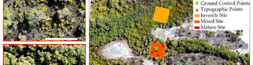
Drones 2019, 3, 32                                                                               2 of 18

as trunks and branches [19], has been used to develop less-destructive estimates of AGB. Structural
attributes can be used to estimate carbon storage by developing species-specific allometric equations,
which establish a relationship between easily measurable traits, such as the diameter at breast height
(DBH) and specific gravity (wood density), and AGB [20]. Carbon content can be estimated relatively
simply by multiplying AGB by the carbon concentration, which varies among species, but is generally
between 45.9% and 47.1% in mangroves [11]. Allometric equations have produced good agreement
with destructively harvested data [11], however, still require intensive field surveys and initial
harvesting [20], and may not be representative of the regional species distribution [21,22]. Therefore,
non-destructive estimates of AGB are being adopted using remote sensing technology that allows the
rapid capture of forest structure, without substituting the level of accuracy needed to inform carbon
accounts [23].
      The use of light detection and ranging (LiDAR) has become common practice for capturing forest
structure to estimate AGB [24]. Full-waveform LiDAR measures the shape of the pulse along its
transmission path as it interacts with surrounding objects [25]. Full-waveform LiDAR sensors may
be attached to aircraft, referred to as airborne laser scanning (ALS), or attached to ground-based
platforms, referred to as terrestrial laser scanning (TLS) [23]. ALS is commonly adopted for large scale
forest inventories, often capturing around 2 to 20 points per m−2 depending on the sensor [24],
whereas TLS scanners are often utilised for plot scale assessments and can capture up to ~1 million
points per second [22], providing upwards of 1000 points per m−2 [26]. TLS can also capture a wealth
of structural information to estimate AGB that shows good agreement with destructively harvested
biomass [27]. However, TLS scanners can cost up to $35,000 USD [28], and surveying and processing
times can be burdensome [26].
      LiDAR sensors attached to unmanned aerial vehicles (UAVs) may offer a more cost-effective
alternative to TLS, while also increasing the spatial and temporal resolution of traditional ALS [28].
However, suitable inertial measuring units (IMUs) and a global navigation satellite system (GNSS)
are required for accurate positioning [23], making commercially available UAV systems costly [29].
      An alternative to LiDAR is the use of structure-from-motion (SfM) technology [30], which has
been used to estimate AGB across a variety of ecosystems [31-34]. The SfM method is a
photogrammetric workflow that uses computer matching of common points in overlapping two-
dimensional images to produce a three-dimensional (3D) point cloud, which is increased in
magnitude using a multi-view stereo (SfM-MVS) [30]. This workflow can be utilised with
photographs taken on-ground, referred to as ‘terrestrial close-range photogrammetry’ [35], which has
been successful for estimating AGB [33] and tree volume [36,37] for forest inventories. However,
given the muddy and inaccessible terrain associated with mangroves, UAVs may represent a more
attractive alternative.
      UAV derived imagery combined with SfM-MVS algorithms provide an inexpensive method for
estimating AGB in forested environments [31,38-40]. This method can acquire accurate estimates of
forest structural attributes, such as tree height, DBH, and stem volume, remotely [34,41–43]. Although
extensive work has been undertaken in forestry [44], applications of SfM-MVS in coastal
environments are limited [45–47]. Only one study at the time of writing has used UAV-derived SfM-
MVS to estimate AGB in mangroves, however, only the upper canopy was observed [43]. It is
unknown how well this technique captures forest structure below the canopy in mangrove
ecosystems when compared with a more established ground-based survey method, such as TLS.
      The objective of this study is to assess the efficacy of using SfM-MVS for capturing forest
structure in three mangrove sites with differing structural characteristics. Given applications of SfM-
MVS have been mainly conducted in forestry plantations characterized by tree stands of regular
height and spacing, we were interested to see how this method would perform in mangroves, which
have more peculiar growth form. Comparisons of point cloud utility is made between SfM-MVS and
TLS, and canopy height models (CHMs) are generated to estimate forest volume as a proxy for AGB.
The findings of this study can be used to inform future applications of the SfM-MVS technique and
whether it is viable for capturing detailed mangrove forest structure to inform AGB estimations.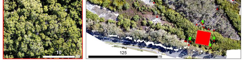
Drones 2019, 3, 32 3 of 18
2. Materials and Methods
2.1. Study Area
Noosa Heads is a small coastal town located roughly 100 km north of Brisbane, Queensland. The
region is sub-tropical, experiencing ~1400 mm precipitation per year, mostly during November to
March [48]. The town is bounded to the north by the Noosa River, a complex river system that
originates near Mount Elliot and extends ~74 km south-east before entering the Pacific Ocean between
Noosa Heads and the southern tip of the Great Sandy National Park (Figure 1). The study area is
located within the Weyba Creek Conservation Park between Lake Weyba and the Noosa River
estuary (Figure 1).
(a) (d) (e)
(b)
(g) (f)
(c)
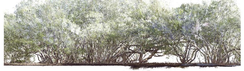
Figure 1. Aerial views of the (a) juvenile, (b) mixed, and (c) mature sites, geographic location in
relation to the (d) Noosa River system and (e) greater Queensland, (f) location of sites and survey
points in study area, and (g) example of a black and white marker.
2.2. Survey Sites
Three 25 × 25 m sites were delineated on the 15 August 2018 to capture the structural attributes
associated with increasing stand age and included: (a) ‘Juveniles’: Mostly seedlings and juveniles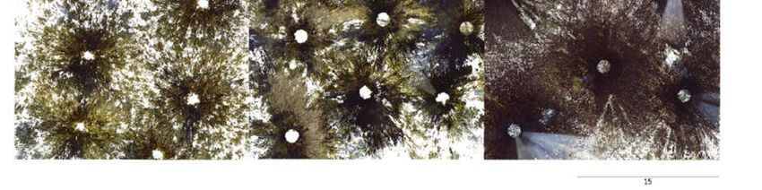
Drones 2019, 3, 32                                                                              4 of 18

2.5 m (Figure 1). Field characterization was conducted using an
inclinometer to obtain tree heights, and mangrove species were identified using descriptions from
[49]. The juvenile site was dominated by a dense population of juvenile Aegicerus corniculatum (River
Mangrove) ranging from 0.7 to 1.5 m tall with scattered Avicennia marina var. australasica (Grey
Mangrove) at around 3.5 m tall. The mixed site contained the same species, but was less dense, with
larger spacings between individual A. marina var. australasica trees and scattered juvenile A.
corniculatum shrubs growing at similar heights as the juvenile site. This site also had a thick matting
of Sporobolus virgincus (Saltcouch) covering the ground surface. The mature site was dominated by
mature age A. marina var. australasica trees growing up to around 8 m tall with a dense canopy and
ground surface covered by pneumatophore roots.

2.3. Field Surveys
      A CHC X91+ Real-Time-Kinetic GNSS (RTK-GNSS), which has a horizontal and vertical
precision of up to 8 mm and 15 mm, respectively [50], was used to obtain 45 Topographic Points
(Figure 1). From these points, 11 ground control points were chosen near the borders of each site, and
these positions were flagged using black and white markers, so they were visible in the subsequent
UAV survey (Figure 1).
      A consumer-grade DJI Phantom 4 Advanced quadcopter was used to obtain 591 overlapping
images of the entire study site. The drone was mounted with a 1” CMOS (complementary metal-
oxide semiconductor) sensor, with an effective pixel size of 20 megapixels, and images were taken at
a resolution of 5472 × 3648 in the RGB (red-green-blue) spectrum using the FC6310 camera (8.8 mm)
[51]. The Ground Station Pro App (DJI, version 2.0) was used to plan the flight, which utilised an
orthogonal flight path and image overlap of 90% forward and 60% side overlap (Figure 2). The flight
was conducted at an average of 51.6 m above ground level, which resulted in a ground sampling
distance (GSD) of 1.38 cm per pixel over an area of 0.07 km2. We used automatic take-off and landing
for the flight, which took 20 minutes and was conducted at 0830 hours Australian Eastern Standard
Time (AEST) on the 30 August 2018, with fine weather and light winds.

      Figure 2. DJI Phantom 4 Advanced quadcopter and flying pattern indicating the number of
      overlapping images, obtained from Agisoft PhotoScan (version 1.5.0).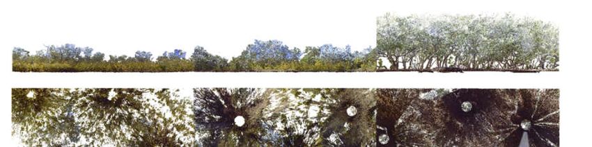
Drones 2019, 3, 32                                                                                          5 of 18

      We used a Faro Focus3D S 120 TLS scanner, which projects constant infrared waves of differing
length outward until they contact an object and are reflected back. Distance is measured by detecting
phase shifts in the infrared waves, and Cartesian coordinates (x, y, z) are recorded. The ranging unit
is capable of capturing points up to 120 m away, with a ranging error of ±2 mm within 25 m using
the factory defined settings. We used a multi-scan approach to capture the forest structure in each
site (Figure 3a–c). To co-register individual scans into a single point cloud, we used a minimum of
three spheres or checkerboard targets in each scan. Targets were placed in open areas to allow the
best possible visibility (Figure 3d,e). The number of scans required per site was determined in the
field, which was dependent on the characteristics of the site and the visibility of the targets. For
example, seven scans were required in the juvenile site, where dense understory vegetation blocked
direct sight between some targets, whereas the mature site only required six scans as targets were
easily visible. All scans were conducted in fine weather, however, when scanning the juvenile site,
wind gusts up to 19 knots were recorded nearby.

(a)                                      (b)                                  (c)

 (d)                                                                (e)                               15m

       Figure 3. Locations of terrestrial laser scanning locations for (a) Juvenile, (b) mixed, and (c) mature
       sites; (d) checkerboard and sphere targets in the juvenile site; and (e) the TLS scanner alongside the
       sphere target in the mature site.

2.4. Data Processing
     The UAV and TLS field surveys were uploaded to the relevant software to process the point
cloud data (Figure 4).
     The UAV data was uploaded into Agisoft Photoscan Professional (version 1.4.3, 64-bit) and was
batch processed at ‘high quality’. The model used all 591 images to create a dense point cloud using
automatic mesh reconstruction. The model was georeferenced in PhotoScan to the Geocentric Datum
of Australia (GDA) 1994 Map Grid of Australia (MGA) Zone 56 using the 11 GCP points, and the
batch process was re-run after camera optimization (non-linear corrections). The TLS data was
imported into FARO Scene (version 5.3) for pre-processing and point cloud registration. Target
spheres were identified in the hemispherical photos and given the corresponding Universal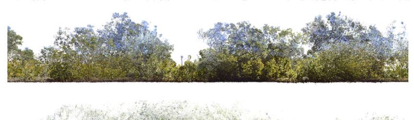
Drones 2019, 3, 32                                                                                   6 of 18

Transverse Mercator (UTM) coordinates in the GDA 94 MGA Zone 56 reference system, which were
obtained by offsetting from GCPs surveyed with the RTK-GNSS. Checkerboard targets were used to
co-register individual scans into a single point cloud for each site using the default origin (0, 0, 0) in
Faro SCENE (v5.3). The TLS point clouds were clipped to a 625 m2 area using a virtual bounding box
and both the SfM-MVS and TLS point clouds were imported into CloudCompare (v2.10. alpha, 64
bit) for rasterization.

      Figure 4. Data processing for UAV and TLS surveys, including software used, processing steps,
      optimization, and final product. * Indicates beginning of structure-from-motion multi-view stereo
      processing.

     The point clouds were segmented using a single transect across each site for both methods to
examine profile point densities and canopy penetration. All point clouds were converted to a digital
surface model (DSM) using the ‘Rasterize’ tool in CloudCompare using the maximum z values and
a cell resolution of 3 cm2, with eight DSMs created in total. Two DSMs were created from the SfM-
MVS survey that spanned the entire study site, and six DSMs were created from the TLS survey that
were confined to the 625 m2 area of each mangrove site. Half of the created DSMs had empty cells
interpolated using the average height value, while the other half were not interpolated. This allowed
an estimation of coverage by dividing the empty cell DSM by the interpolated DSM and multiplying
by 100.

2.5. Volume Calculation
     A volumetric or surface differencing approach was used to estimate mangrove forest volume,
which involves subtracting a DTM from a DSM to obtain a CHM, thereby normalizing object heights
above ground [52]. Forest volume, which includes all pixels associated with aboveground vegetation,
can then be estimated by multiplying the canopy height value of a raster cell by its resolution [53,54].
A DTM was created in ArcMap (version 10.6) by interpolating all 45 topographic points with the
‘Topo to Raster’ tool (Figure 5).
     In ArcMap, the SfM-MVS DSM was projected to the GDA 94 MGA Zone 56 reference system
and the Australian Height Datum (AHD). The TLS DSMs were imported with z elevation, but no x
or y coordinates, due to a truncation issue with the global coordinates in FARO Scene. Therefore, the
TLS DSMs were also projected into the GDA 94 MGA Zone 56 and AHD reference systems, and
subsequently georeferenced to the same coordinates as the SfM-MVS DSMs manually in ArcMap.
During the rasterisation process, it was noted that some point clouds contained spurious points
below ground height, which carried over into the raster model. Therefore, these were corrected using
a conditional raster that changed their value to zero. Once the per cell volume was calculated, the
sum of all cells contained within each site gave the estimated forest volume in cubic metres (m3).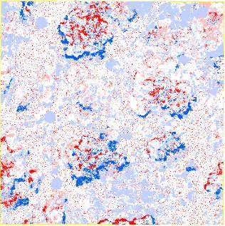
Drones 2019, 3, 32                                                                                7 of 18

      Figure 5. Volume calculation workflow conducted in ArcMap. Note this workflow was repeated for
      both SfM-MVS and TLS across all three sites, making six iterations in total.

    The raster models were converted to point files and the mean absolute error (MAE) for canopy
height models and volume estimations were calculated using the equation:

                                               =       |   −ŷ |

where n is the number of observations, yj is the observed value, and ŷj is the predicted value calculated
for each observation.
     The differences in volume were also expressed as a percentage using the equation:
                     Percentage difference = 100*|TLS – SfM-MVS/((TLS + SfM-MVS)/2)
     Finally, the CHMs were reclassified so that only vegetation greater than 1.37 m was displayed,
which produced a rough estimate of canopy cover. The SfM-MVS volume raster was subtracted from
the TLS volume raster to identify the spatial distribution of differences in forest volume.

3. Results

3.1. Point Clouds
     The point cloud derived from the SfM-MVS process can be seen in Figure 6.
     The SfM point matching used 336,195 tie points to create a sparse point cloud, which was
increased to 162,196,895 points using MVS over an area of 67,292.19 m2, with white pixels indicating
areas of no data (Figure 6). The side view of the SfM-MVS revealed spurious low points that were
most evident in the eastern side of the study area (Figure 6). A side profile view of the TLS surveys
indicates high point density in understory vegetation, with some gaps evident in the canopy,
especially in the mature site (Figure 7). Spurious low points were also evident in the TLS scans,
especially in the mature site (Figure 7).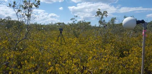
Drones 2019, 3, 32                                                                                     8 of 18

a)

b)

                     100m

      Figure 6. Point cloud of the entire study area derived from high resolution unmanned aerial vehicle
      imagery and SfM-MVS processing viewed from (a) an aerial angle and (b) a horizontal angle. Note
      the red circle indicates spurious low points.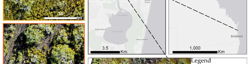
Drones 2019, 3, 32                                                                                           9 of 18

  a)

  b)
                                                                                               6.5m

  c)

             6.5m
       Figure 7. Horizontal profile of TLS point clouds for (a) juvenile, (b) mixed, and (c) mature sites. Note
       the red circle indicates spurious low points.

       A comparison of methods in terms of survey and processing time can be seen in Table 1.

            Table 1. Time required for surveys and data processing and number of points per 625 m2.

                               SfM-MVS                                     TLS
                               Study area            Juvenile           Mixed             Mature
       No. of scans                 1                    7                 8                 6
       Survey time             20 minutes           3.5 hours           3 hours          2.5 hours
     Processing time1           37 hours             2 hours           1.5 hours         1.5 hours
     Points per 625m2           1,506,426           66,520,190       121,085,632        147,995,632
 Computer specifications: Laptop: Dell Precision 5520 i7-7820HQ CPU @ 2.90 GHz 32 GB RAM, Graphics
 Processing Unit (GPU) Quadro M1200
*Note all times are approximate. 1Processing time includes time spent co-registering scans manually for TLS,
which took longer in the juvenile site due to dense vegetation.

     Survey time was lower for the SfM-MVS than the TLS surveys, with all data collected by the
UAV in roughly 20 minutes (Table 1). The final point clouds for the TLS produced up to ~100 times
more points compared to SfM-MVS, with the highest and lowest number of points recorded in the
mature and juvenile sites, respectively (Table 1). More scans did not necessarily correspond to more
registered points, as the mature site had the most points, but fewest scans (Table 1). Scanning
coverage differed between all sites as seen in Figure 8.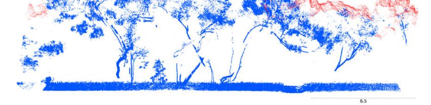
Drones 2019, 3, 32                                                                                             10 of 18

    a)                                       b)                                  c)
                                                                                                         15m
           Figure 8. Coverage for different scanner positions from the TLS surveys using a ‘bottom up’ view in
           the (a) juvenile, (b) mixed, and (c) mature sites.

     Fewer empty cells were visible in the mature site compared to the juvenile and mixed sites,
resulting in greater overall coverage (Figure 8). The results of the point cloud rasterization and
coverage calculations can be seen in Table 2.

                                      Table 2. Summary of the rasterization process.

                                                         TLS                               SfM-MVS
                                              Juvenile    Mixed       Mature      Juvenile     Mixed      Mature
                     Area (m2)1                 620.75     633.33      621.24       619.81     633.34     621.24
          No. of cells (no interpolation)2     506,264    587,899     680,271      630,627     652,552    592,796
           No. of cells (interpolation)3       689,726    703,702     690,263      688,673     703,705    690,266
                   Coverage (%)                  73.40     83.54       98.55        91.57       92.73      85.88
1, 2, 3
     Note slight differentiation in site boundaries led to differences in the total area and cell numbers for each
site, as noted above.

     The lowest and highest cell coverage occurred for the TLS scans in the juvenile and mature sites,
respectively (Table 2). The SfM-MVS method produced less variation in cell coverage compared to
the TLS (Table 2). Profiles derived from segments of the point clouds can be seen in Figure 9.
     Tree stems, foliage, and the ground surface were well represented in the mature site (Figure 9).
Point densities appear to decrease within dense vegetation across all sites, including the TOC and at
ground level (Figure 9). Ground points were under-represented using the SfM-MVS method,
including areas below dense vegetation or canopy (Figure 9). It was also noted that the TLS registered
several points in ‘mid-air’ that were not captured by the SfM-MVS method, which was most evident
in the juvenile and mixed sites (Figure 9).
Drones 2019, 3, 32 11 of 18
a) TLS SfM-MVS
b)
c)
15m
Figure 9. Horizontal profile of point clouds compared between methods and (a) juvenile, (b) mixed,
and (c) mature sites.
3.2. Forest Volume
The SfM-MVS method produced lower maximum cell heights than TLS for all sites after
rasterization (Table 3).
Table 3. Descriptive statistics for digital surface models across sites and survey methods.
TLS SfM-MVS
Juvenile Mixed Mature Juvenile Mixed Mature
Max height (m) 3.88 4.70 8.66 3.45 4.01 8.27
Avg. max. height (m) 1.09 0.94 4.51 0.71 0.71 5.11
(Std. Dev.) (0.52) (0.91) (2.11) (0.57) (0.93) (1.75)
Volume (m3) 679 596 2800 439 448 3180
The average maximum heights were lower for the SfM-MVS method in the juvenile and mixed
sites, and higher in the mature site when compared with TLS (Table 3). This corresponded to lower
measures of volume in the juvenile and mixed sites, but higher volume in the mature site for SfM-
MVS (Table 3). The error calculated between the methods for canopy height and volume estimates
can be seen in Table 4.
The highest MAEs for both the CHM and volume estimation were observed in the mature site,
and the lowest were observed in the mixed site (Table 4). The lowest percentage difference in volume
was recorded in the mature site, despite having the greatest error (Table 4). The highest percentage
difference in volume was recorded in the juvenile site, with the mixed site also reporting a substantialDrones 2019, 3, 32 12 of 18
difference in volume estimation (Table 4). The TLS-derived canopy cover was 20.03% in the juvenile
site, 30.91% in the mixed site, and 84.15% in the mature site (Figure 10a–c).
Table 4. Mean absolute error and percentage difference between TLS and SfM-MVS.
Juvenile Mixed Mature
CHM—MAE 0.39 m 0.23 m 0.61 m
Volume—MAE 3.47 × 10⁻⁴ m3 2.10 × 10⁻⁴ m3 5.50 × 10⁻⁴ m3
Volume—Percent diff.1 42.95% 28.23% 12.72%
1 Note percent difference was calculated as the deviation of SfM-MVS from TLS measurements.
a) b) c)
d) e) f)
Figure 10. Canopy cover as measured by the TLS for the (a) juvenile, (b) mixed, and (c) mature site,
and volume differences in the (d) juvenile, (e) mixed, and (f) mature site. Note blue colours indicate
higher TLS estimates while red indicates lower TLS estimates when compared to SfM-MVS.
Differences in volume between the juvenile, mixed, and mature sites can be seen in Figure 10d–
f. The TLS produced greater measures of volume for vegetation below 1.37 m, as indicated by the
prevalence of blue cells in those sites (Figure 10d,e). In the mature site, the greatest volume differences
generally corresponded to canopy gaps, with the SfM-MVS recording greater heights in these areas
compared to the TLS (Figure 10f).
4. Discussion
4.1. Point Cloud Density and Forest Structure
In general, the UAV point cloud was obtained much faster than the TLS point clouds, and
despite having a greater overall processing time, much of this was automated and required little
input, which was comparable with other studies [28,46]. The time taken to conduct traditional AGB
assessments in mangroves is not often reported, however, survey periods generally extend acrossDrones 2019, 3, 32 13 of 18
several months depending on the size and complexity of the site. This is generally related to the
muddy and/or inaccessible terrain and the desire to minimise damage from trampling
pneumatophore roots and seedlings [11]. By comparison, the 20-minute UAV flight or multi-day
survey conducted with the TLS in this study required substantially less time in the field compared to
traditional methods. The final TLS point clouds contained approximately 45 to 100 times more points
per/625 m2 than the SfM-MVS point clouds across all sites. Point density of this magnitude is not
uncommon using TLS [26,53], and the lower point density for SfM-MVS is likely linked to the survey
settings. For example, flying at a lower altitude or increasing the degree of image overlap can greatly
increase point density [55]. However, it should be considered whether the greater point density
offered by the TLS is worth spending more time in the field, increasing the potential of trampling
damage.
High stem density in the juvenile site likely led to poor cell coverage and capture of forest
structure, whereas a low stem density in the mature site allowed greater capture of forest structure.
Occlusion is a commonly reported limitation of using TLS in vegetated environments [56], which can
lead to highly variable point densities [23,28,57,58]. This was partially controlled for by incorporating
multiple scans well within the optimal 25 m radius from the scanner, however, laser pulses were still
unable to penetrate fully through dense vegetation. The higher average cell coverage for SfM-MVS
was likely due to the high redundancy of overlapping images, which ensures sufficient point
matching [46,55], and the high spatial resolution of the imagery. Despite this, the SfM-MVS method
only captured the outer canopy envelope, with many studies linking poor canopy penetration to low
capture of forest structure and/or underlying terrain [39,59-61]. As expected, the ground-based TLS
was better able to capture below canopy forest structure, whereas the aerial-based SfM-MVS was
better equipped to survey canopy height, with neither survey type efficient for both.
4.2. Canopy Height and Volume Estimations
The higher average maximum canopy height for SfM-MVS in the mature site is likely due to
overestimation, which has been found in mangroves [43] and other forested environments
[28,39,59,61]. SfM-MVS is generally unable to represent fine scale canopy gaps [62] and smoothing of
these gaps during rasterization can lead to overestimations of height [23]. This was observed in the
volume difference raster, where greater SfM-MVS volumes tend to correspond to gaps in the canopy
cover. Furthermore, the lower maximum cell height recorded by SfM-MVS in this site is not unusual,
as this method is known to underestimate the maximum height of individual plants [55]. The higher
error recorded in this site, despite having the lowest difference in volume, is likely due to poor TOC
representation for the TLS, which had the highest standard deviation for all sites. Occlusion of TOC
points in TLS scans can produce erroneous canopy height estimations [63], with a low TOC sample
point density corresponding to under-estimations of canopy height in other studies [18]. It is
important to note all AGB estimations carry some degree of error. For example, the departure of
allometric models, which are generally considered more robust, from measured field data has been
reported as high as 49.2% for estimations of AGB [20], and 18.4% for estimations of volume [64] in
mangroves, which varies between the species and equations used.
Conversely, the average maximum canopy height was lower for the juvenile and mixed sites,
which also had high variation between volume estimations. This was likely a function of the dense
understory layer in the juvenile site, as high stem density can lead to poor point capture for both SfM-
MVS [65] and TLS [23]. For the TLS measurements, greater recorded heights and subsequent volume
may be a function of artificial mid-air points that result from beam interceptions at the canopy edge,
which can affect height estimations [28,56]. In this case, beam interceptions may have occurred
horizontally, where taller shrubs occluded shorter ones, producing spurious high points. For the SfM-
MVS, it is possible that high stem density led to poor image matching, which can lead to
underestimations of DSM heights [32]. Alternatively, wind gusts can cause outer branches to move
between images, leading to feature rejection during image matching [55], which would explain the
poor representation of higher points by SfM-MVS in the juvenile site. Similar effects may have
occurred in the mixed site, however, the difference in error and volume were likely reduced due toDrones 2019, 3, 32 14 of 18
decreased stem density. For example, SfM-MVS is more likely to match LiDAR data in sparsely
vegetated areas [65,66], and error decreases with increasing bare area [67]. Similarly, occlusion is less
of an issue for TLS scans in sparsely vegetated environments [58]. The greatest differences between
SfM-MVS and TLS in this site occurred in the TOC and at the canopy edge, which suggests occlusion
and beam interceptions may have hindered point capture in these dense areas.
4.3. Limitations and Future Considerations
Comparison between the canopy cover raster and the volume difference raster highlighted
horizontal misalignments between the TLS and SfM-MVS raster models. This was greatest in the
juvenile and mixed sites, where canopy edges tend to ‘shadow’ each other. This is an artefact of the
georeferencing process, which had to be performed manually in ArcMap. Horizontal co-registration
error for canopy heights are generally small [68], but vertical co-registration of CHMs and DTMs
obtained from different data sources remains a major challenge when estimating canopy heights [55].
In this case, DSMs and DTMs were aligned vertically using the AHD projection, but models were
imperfectly aligned horizontally, which may have led to differences in volume estimations.
Differences may have also stemmed from spurious high points as mentioned previously. This could
likely be resolved by using a point filtering algorithm to remove outliers, or by using a percentile of
a cell’s elevation rather than the maximum z value, as this can make CHMs less sensitive to outliers
[39,66].
The surface differencing method requires an accurate high spatial resolution DTM to normalize
canopy heights above ground [23,69]. The DTM created in this study interpolated elevation heights
that were taken at the peripheries of each site, since the RTK-GNSS could not obtain a signal below
the canopy. This is less of an issue in small level plots, as changes in topography are expected to be
minimal [28]. However, any upscaling of this method would require a more representative DTM. The
surface differencing method also assumes a constant volume below the height of the CHM [53]. Each
site contained mangrove species with different growth forms at differing stem densities.
Furthermore, wood density in mangroves is species-specific [11,12], meaning the AGB across each
site is not constant and will differ depending on the species composition. Therefore, sites that contain
a higher stem density that are dominated by a single species, such as the juvenile site, likely represent
a more accurate estimation of volume using this method.
5. Conclusions
This study compared the ability of SfM-MVS and TLS to capture forest structure and volume in
three mangrove sites of differing structural characteristics. For forest structure, SfM-MVS was unable
to capture points below the canopy in the same detail offered by TLS, which was clearly superior in
terms of point density. For forest volume, SfM-MVS captured the top of the canopy more accurately
than the TLS, which suffered from occlusion, however, it tends to overestimate volume in canopy
gaps. Furthermore, increasing stem density led to the capture of erroneous points for both SfM-MVS
and TLS, suggesting either method may be more appropriate in lower density mangroves.
In summary, we suggest TLS would be more beneficial for capturing mangrove forest structure,
whereas SfM-MVS would be better for capturing mangrove canopy height, and subsequent volume.
However, the choice between either SfM-MVS and TLS depends on the accuracy, spatial scale, and
time scale required, with both offering potential advantages and disadvantages. Our results could
better inform future work in the conservation of these important ecosystems, given the rapid decline
of mangroves globally.
Author Contributions: All work conducted by Angus Warfield and Javier Leon.
Funding: This research received no external funding.
Acknowledgments: We would like to acknowledge the School of Science and Engineering at the University of
the Sunshine Coast, Queensland, for supporting our research.
Conflicts of Interest: The authors declare no conflict of interest.Drones 2019, 3, 32 15 of 18
References
1. Giri, C.; Ochieng, E.; Tieszen, L.L.; Zhu, Z.; Singh, A.; Loveland, T.; Masek, J.; Duke, N. Status and
distribution of mangrove forests of the world using earth observation satellite data. Glob. Ecol. Biogeogr.
2011, 20, 154–159.
2. Mackenzie, J.R.; Duke, N.C.; Wood, A.L. The Shoreline Video Assessment Method (S-VAM): Using
dynamic hyperlapse image acquisition to evaluate shoreline mangrove forest structure, values,
degradation and threats. Mar. Pollut. Bull. 2016, 109, 751–763, doi:10.1016/j.marpolbul.2016.05.069.
3. Cuc, N.T.K.; Suzuki, T.; de Ruyter van Steveninck, E.D.; Hai, H. Modelling the Impacts of Mangrove
Vegetation Structure on Wave Dissipation in Ben Tre Province, Vietnam, under Different Climate Change
Scenarios. J. Coast. Res. 2015, 31, 340–347.
4. Thomas, N.; Bunting, P.; Lucas, R.; Hardy, A.; Rosenqvist, A.; Fatoyinbo, T. Mapping Mangrove Extent and
Change: A Globally Applicable Approach. Remote Sens. 2018, 10, 1466.
5. Donato, D.C.; Kauffman, J.B.; Murdiyarso, D.; Kurnianto, S.; Stidham, M.; Kanninen, M. Mangroves among
the most carbon-rich forests in the tropics. Nature Geosci. 2011, 4, 293, doi:10.1038/ngeo1123
6. Duarte, C.M.; Middelburg, J.J.; Caraco, N. Major role of marine vegetation on the oceanic carbon cycle.
Biogeosci. Discuss. 2005, 1, 659–679.
7. Alongi, D.M. Present state and future of the world's mangrove forests. Environ. Conserv. 2002, 29, 331–349,
doi:10.1017/S0376892902000231.
8. Alongi, D.M. Carbon Cycling and Storage in Mangrove Forests. Annu. Rev. Mar. Sci. 2014, 6, 195–219,
doi:10.1146/annurev-marine-010213-135020.
9. Thomas, N.; Lucas, R.; Bunting, P.; Hardy, A.; Rosenqvist, A.; Simard, M. Distribution and drivers of global
mangrove forest change, 1996–2010. PloS One 2017, 12, e0179302.
10. Atwood, T.; Connolly, R.; Almahasheer, H.; Carnell, P.; Duarte, C.; Ewers Lewis, C.; Irigoien, X.; Kelleway,
J.; Lavery, P.; Macreadie, P.; et al. Global patterns in mangrove soil carbon stocks and losses. Nat. Clim.
Chang. 2017, 7, 523, doi:10.1038/nclimate3326.
11. Kauffman, J.B.; Donato, D.C. Protocols for the Measurement, Monitoring and Reporting of Structure, Biomass,
and Carbon Stocks in Mangrove Forests; Center for International Forestry Research (CIFOR), Bogor, Indonesia,
2012.
12. Howard, J., Hoyt, S., Isensee, K., Telszewski, M., Pidgeon, E., Eds. Coastal Blue Carbon: Methods for Assessing
Carbon Stocks and Emissions Factors in Mangroves, Tidal Salt Marshes, and Seagrasses; Conservation
International, Intergovernmental Oceanographic Commission of UNESCO, International Union for
Conservation of Nature: Arlington, VA, USA, 2014; pp. 180.
13. Mcleod, E.; Chmura, G.L.; Bouillon, S.; Salm, R.; Björk, M.; Duarte, C.M.; Lovelock, C.E.; Schlesinger, W.H.;
Silliman, B.R. A blueprint for blue carbon: Toward an improved understanding of the role of vegetated
coastal habitats in sequestering CO2. Front. Ecol. Environ. 2011, 9, 552–560.
14. Feliciano, E.A.; Wdowinski, S.; Potts, M.D. Assessing Mangrove Above-Ground Biomass and Structure
using Terrestrial Laser Scanning: A Case Study in the Everglades National Park. Wetlands 2014, 34, 955–
968, doi:10.1007/s13157-014-0558-6.
15. Kauffman, J.B.; Heider, C.; Cole, T.G.; Dwire, K.A.; Donato, D.C. Ecosystem Carbon Stocks of Micronesian
Mangrove Forests. Wetlands 2011, 31, 343–352, doi:10.1007/s13157-011-0148-9.
16. Watt, P.J.; Donoghue, D.N.M. Measuring forest structure with terrestrial laser scanning. Int. J. Remote Sens.
2005, 26, 1437–1446, doi:10.1080/01431160512331337961.
17. Mascaro, J.; Asner, G.; Davies, S.; Dehgan, A.; Saatchi, S. These are the days of lasers in the jungle. Carbon
Balance Manag. 2014, 9, 1–3, doi:10.1186/s13021-014-0007-0.
18. Hopkinson, C.; Chasmer, L.; Colin, Y.-P.; Treitz, P. Assessing forest metrics with a ground-based scanning
lidar. Can. J. For. Res.2004, 34, 573–583, doi:10.1139/X03-225.
19. McElhinny, C.; Gibbons, P.; Brack, C.; Bauhus, J. Forest and woodland stand structural complexity: Its
definition and measurement. For. Ecol. Manag. 2005, 218, 1–24,
doi:https://doi.org/10.1016/j.foreco.2005.08.034.
20. Chave, J.; Andalo, C.; Brown, S.; Cairns, M.A.; Chambers, J.Q.; Eamus, D.; Fölster, H.; Fromard, F.; Higuchi,
N.; Kira, T.; et al. Tree allometry and improved estimation of carbon stocks and balance in tropical forests.
Oecologia 2005, 145, 87–99, doi:10.1007/s00442-005-0100-x.Drones 2019, 3, 32 16 of 18
21. Van Breugel, M.; Ransijn, J.; Craven, D.; Bongers, F.; Hall, J.S. Estimating carbon stock in secondary forests:
Decisions and uncertainties associated with allometric biomass models. For. Ecol. Manag. 2011, 262, 1648–
1657, doi:https://doi.org/10.1016/j.foreco.2011.07.018.
22. Liang, X.; Kankare, V.; Hyyppä, J.; Wang, Y.; Kukko, A.; Haggrén, H.; Yu, X.; Kaartinen, H.; Jaakkola, A.;
Guan, F.; et al. Terrestrial laser scanning in forest inventories. ISPRS J. Photogramm. Remote Sens. 2016, 115,
63–77, doi:10.1016/j.isprsjprs.2016.01.006.
23. White, J.C.; Coops, N.C.; Wulder, M.A.; Vastaranta, M.; Hilker, T.; Tompalski, P. Remote Sensing
Technologies for Enhancing Forest Inventories: A Review. Can. J. Remote Sens. 2016, 42, 619–641,
doi:10.1080/07038992.2016.1207484.
24. Masek, J.G.; Hayes, D.J.; Joseph Hughes, M.; Healey, S.P.; Turner, D.P. The role of remote sensing in
process-scaling studies of managed forest ecosystems. For. Ecol. Manag. 2015, 355, 109–123,
doi:10.1016/j.foreco.2015.05.032.
25. Yang, X.; Strahler, A.H.; Schaaf, C.B.; Jupp, D.L.; Yao, T.; Zhao, F.; Wang, Z.; Culvenor, D.S.; Newnham,
G.J.; Lovell, J.L. Three-dimensional forest reconstruction and structural parameter retrievals using a
terrestrial full-waveform lidar instrument (Echidna®). Remote Sens. Environ. 2013, 135, 36–51.
26. Olsoy, P.J.; Glenn, N.F.; Clark, P.E.; Derryberry, D.R. Aboveground total and green biomass of dryland
shrub derived from terrestrial laser scanning. ISPRS J. Photogramm. Remote Sens. 2014, 88, 166–173,
doi:10.1016/j.isprsjprs.2013.12.006.
27. Calders, K.; Newnham, G.; Burt, A.; Murphy, S.; Raumonen, P.; Herold, M.; Culvenor, D.; Avitabile, V.;
Disney, M.; Armston, J.; et al. Nondestructive estimates of above-ground biomass using terrestrial laser
scanning. Methods Ecol. Evol. 2015, 6, 198–208, doi:10.1111/2041-210X.12301.
28. Wallace, L.; Hillman, S.; Reinke, K.; Hally, B. Non-destructive estimation of above-ground surface and
near-surface biomass using 3D terrestrial remote sensing techniques. Methods Ecol. Evol. 2017, 8, 1607–1616,
doi:10.1111/2041-210X.12759.
29. Wallace, L.; Lucieer, A.; Watson, C.; Turner, D. Development of a UAV-LiDAR System with Application to
Forest Inventory. Remote Sens. 2012, 4, 1519.
30. Smith, M.W.; Carrivick, J.L.; Quincey, D.J. Structure from motion photogrammetry in physical geography.
Prog. Phys. Geogr. Earth Environ. 2015, 40, 247–275, doi:10.1177/0309133315615805.
31. Messinger, M.; Asner, G.; Silman, M. Rapid Assessments of Amazon Forest Structure and Biomass Using
Small Unmanned Aerial Systems. Remote Sens. 2016, 8, 615.
32. Koci, J.; Jarihani, B.; Leon, J.X.; Sidle, R.; Wilkinson, S.; Bartley, R. Assessment of UAV and Ground-Based
Structure from Motion with Multi-View Stereo Photogrammetry in a Gullied Savanna Catchment. ISPRS
Int. J. Geo-Inf. 2017, 6, 328.
33. Cooper, S.; Roy, D.; Schaaf, C.; Paynter, I. Examination of the Potential of Terrestrial Laser Scanning and
Structure-from-Motion Photogrammetry for Rapid Nondestructive Field Measurement of Grass Biomass.
Remote Sens. 2017, 9, 531.
34. Alonzo, M.; Andersen, H.-E.; Morton, D.; Cook, B. Quantifying Boreal Forest Structure and Composition
Using UAV Structure from Motion. Forests 2018, 9, 119.
35. Niederheiser, R.; Mokros, M.; Lange, J.; Petschko, H.; Prasicek, G.; Elberink, S.O. Deriving 3D point clouds
from terrestrial photographs comparison of different sensors and software. In Proceedings of the XXIII ISPRS
Congress, Prague, Czech Republic, 12–19 July 2016; pp. 685–692.
36. Miller, J.; Morgenroth, J.; Gomez, C. 3D modelling of individual trees using a handheld camera: Accuracy
of height, diameter and volume estimates. Urban For. Urban Green. 2015, 14, 932–940.
37. Mikita, T.; Janata, P.; Surový, P. Forest stand inventory based on combined aerial and terrestrial close-range
photogrammetry. Forests 2016, 7, 165.
38. Puliti, S.; Ørka, H.; Gobakken, T.; Næsset, E. Inventory of Small Forest Areas Using an Unmanned Aerial
System. Remote Sens. 2015, 7, 9632–9654.
39. Zahawi, R.A.; Dandois, J.P.; Holl, K.D.; Nadwodny, D.; Reid, J.L.; Ellis, E.C. Using lightweight unmanned
aerial vehicles to monitor tropical forest recovery. Biol. Conserv. 2015, 186, 287–295,
doi:https://doi.org/10.1016/j.biocon.2015.03.031.
40. Thiel, C.; Schmullius, C. Comparison of UAV photograph-based and airborne lidar-based point clouds
over forest from a forestry application perspective. Int. J. Remote Sens. 2017, 38, 2411–2426,
doi:10.1080/01431161.2016.1225181.Drones 2019, 3, 32 17 of 18
41. Abdollahnejad, A.; Panagiotidis, D.; Surový, P. Estimation and Extrapolation of Tree Parameters Using
Spectral Correlation between UAV and Pléiades Data. Forests 2018, 9, 85.
42. Giannetti, F.; Chirici, G.; Gobakken, T.; Næsset, E.; Travaglini, D.; Puliti, S. A new approach with DTM-
independent metrics for forest growing stock prediction using UAV photogrammetric data. Remote Sens.
Environ. 2018, 213, 195–205, doi:https://doi.org/10.1016/j.rse.2018.05.016.
43. Otero, V.; Van De Kerchove, R.; Satyanarayana, B.; Martínez-Espinosa, C.; Fisol, M.A.B.; Ibrahim, M.R.B.;
Sulong, I.; Mohd-Lokman, H.; Lucas, R.; Dahdouh-Guebas, F. Managing mangrove forests from the sky:
Forest inventory using field data and Unmanned Aerial Vehicle (UAV) imagery in the Matang Mangrove
Forest Reserve, peninsular Malaysia. Forest Ecol. Manag. 2018, 411, 35–45,
doi:https://doi.org/10.1016/j.foreco.2017.12.049.
44. Torresan, C.; Berton, A.; Carotenuto, F.; Di Gennaro, S.F.; Gioli, B.; Matese, A.; Miglietta, F.; Vagnoli, C.;
Zaldei, A.; Wallace, L. Forestry applications of UAVs in Europe: a review. Int. J. Remote Sens. 2017, 38, 2427–
2447, doi:10.1080/01431161.2016.1252477.
45. Bryson, M.; Johnson-Roberson, M.; Murphy, R.J.; Bongiorno, D. Kite Aerial Photography for Low-Cost,
Ultra-high Spatial Resolution Multi-Spectral Mapping of Intertidal Landscapes. PLOS ONE 2013, 8, e73550,
doi:10.1371/journal.pone.0073550.
46. Mancini, F.; Dubbini, M.; Gattelli, M.; Stecchi, F.; Fabbri, S.; Gabbianelli, G. Using Unmanned Aerial
Vehicles (UAV) for High-Resolution Reconstruction of Topography: The Structure from Motion Approach
on Coastal Environments. Remote Sens. 2013, 5, 6880.
47. Lucieer, A.; Turner, D.; King, D.H.; Robinson, S.A. Using an Unmanned Aerial Vehicle (UAV) to capture
micro-topography of Antarctic moss beds. Int. J. Appl. Earth Obs. Geoinf. 2014, 27, 53–62,
doi:https://doi.org/10.1016/j.jag.2013.05.011.
48. B.O.M. Summary Statistics - Sunshine Coast Airport. Availabe online:
http://www.bom.gov.au/climate/averages/tables/cw_040861.shtml (accessed on 19 April 2018).
49. Leiper, G.; Leiper, G. Mangroves to Mountains: a field guide to the native plants of south-east Queensland; Logan
River Branch, Society for Growing Australian Plants (Qld Region): Fortitude Valley, QLD, Australia, 2008.
50. CHC. CHC X91+ Datasheet. Available online:
http://www.chcnav.com/index.php/welcome/search?key=x91%2B (accessed on 15 October 2018).
51. DJI. Phantom 4 Pro V2.0. Availabe online: https://store.dji.com/product/phantom-4-pro-v2?vid=43151
(accessed on 20 October 2018).
52. White, J.C.; Wulder, M.A.; Vastaranta, M.; Coops, N.C.; Pitt, D.; Woods, M. The utility of image-based point
clouds for forest inventory: A comparison with airborne laser scanning. Forests 2013, 4, 518-536.
53. Greaves, H.E.; Vierling, L.A.; Eitel, J.U.H.; Boelman, N.T.; Magney, T.S.; Prager, C.M.; Griffin, K.L.
Estimating aboveground biomass and leaf area of low-stature Arctic shrubs with terrestrial LiDAR. Remote
Sens. Environ. 2015, 164, 26-35, doi:https://doi.org/10.1016/j.rse.2015.02.023.
54. Owers, C.J.; Rogers, K.; Woodroffe, C.D. Terrestrial laser scanning to quantify above-ground biomass of
structurally complex coastal wetland vegetation. Estuarine Coast. Shelf Sci. 2018, 204, 164–176,
doi:https://doi.org/10.1016/j.ecss.2018.02.027.
55. Dandois, J.; Olano, M.; Ellis, E. Optimal Altitude, Overlap, and Weather Conditions for Computer Vision
UAV Estimates of Forest Structure. Remote Sens. 2015, 7, 13895.
56. Newnham, G.; Armston, J.; Muir, J.; Goodwin, N.; Tindall, D.; Culvenor, D.; Püschel, P.; Nyström, M.;
Johansen, K. Evaluation of Terrestrial Laser Scanners for Measuring Vegetation Structure; CSIRO: Perth,
Australia, 2012.
57. Pirotti, F.; Guarnieri, A.; Vettore, A. Ground filtering and vegetation mapping using multi-return terrestrial
laser scanning. ISPRS J. Photogramm. Remote Sens. 2013, 76, 56–63,
doi:https://doi.org/10.1016/j.isprsjprs.2012.08.003.
58. Liang, X.; Hyyppä, J.; Kaartinen, H.; Lehtomäki, M.; Pyörälä, J.; Pfeifer, N.; Holopainen, M.; Brolly, G.;
Francesco, P.; Hackenberg, J., et al. International benchmarking of terrestrial laser scanning approaches for
forest inventories. ISPRS J. Photogramm. Remote Sens. 2018, 144, 137–179,
doi:https://doi.org/10.1016/j.isprsjprs.2018.06.021.
59. Dandois, J.P.; Ellis, E.C. Remote Sensing of Vegetation Structure Using Computer Vision. Remote Sens. 2010,
2, 1157–1176.Drones 2019, 3, 32 18 of 18
60. Wallace, L.; Lucieer, A.; Malenovský, Z.; Turner, D.; Vopěnka, P. Assessment of Forest Structure Using
Two UAV Techniques: A Comparison of Airborne Laser Scanning and Structure from Motion (SfM) Point
Clouds. Forests 2016, 7, 62.
61. Roşca, S.; Suomalainen, J.; Bartholomeus, H.; Herold, M. Comparing terrestrial laser scanning and
unmanned aerial vehicle structure from motion to assess top of canopy structure in tropical forests. Interface
Focus 2018, 8, doi:10.1098/rsfs.2017.0038.
62. Lisein, J.; Pierrot-Deseilligny, M.; Bonnet, S.; Lejeune, P. A Photogrammetric Workflow for the Creation of
a Forest Canopy Height Model from Small Unmanned Aerial System Imagery. Forests 2013, 4, 922.
63. Yu, X.; Liang, X.; Hyyppä, J.; Kankare, V.; Vastaranta, M.; Holopainen, M. Stem biomass estimation based
on stem reconstruction from terrestrial laser scanning point clouds. Remote Sens. Lett. 2013, 4, 344-353,
doi:10.1080/2150704X.2012.734931.
64. Cole, T.G.; Ewel, K.C.; Devoe, N.N. Structure of mangrove trees and forests in Micronesia. Forest Ecol.
Manag. 1999, 117, 95-109.
65. Cook, K.L. An evaluation of the effectiveness of low-cost UAVs and structure from motion for geomorphic
change detection. Geomorphology 2017, 278, 195–208, doi:https://doi.org/10.1016/j.geomorph.2016.11.009.
66. Cunliffe, A.M.; Brazier, R.E.; Anderson, K. Ultra-fine grain landscape-scale quantification of dryland
vegetation structure with drone-acquired structure-from-motion photogrammetry. Remote Sens. Environ.
2016, 183, 129-143, doi:https://doi.org/10.1016/j.rse.2016.05.019.
67. Javernick, L.; Brasington, J.; Caruso, B. Modeling the topography of shallow braided rivers using Structure-
from-Motion photogrammetry. Geomorphology 2014, 213, 166-182, doi:10.1016/j.geomorph.2014.01.006.
68. Frazer, G.; Magnussen, S.; Wulder, M.; Niemann, K. Simulated impact of sample plot size and co-
registration error on the accuracy and uncertainty of LiDAR-derived estimates of forest stand biomass.
Remote Sens. Environ. 2011, 115, 636–649.
69. Muir, J.; Goodwin, N.; Armston, J.; Phinn, S.; Scarth, P. An Accuracy Assessment of Derived Digital
Elevation Models from Terrestrial Laser Scanning in a Sub-Tropical Forested Environment. Remote Sens.
2017, 9, 843.
© 2019 by the authors. Licensee MDPI, Basel, Switzerland. This article is an open access
article distributed under the terms and conditions of the Creative Commons Attribution
(CC BY) license (http://creativecommons.org/licenses/by/4.0/).You can also read